A Comprehensive Study of Nonlinear Mixed Integro-Differential Equations of the Third Kind for Initial Value Problems: Existence, Uniqueness and Numerical Solutions

Abstract

Nonlinear mixed integro-differential equations (NM-IDEs) of the third kind present a complex challenge during solving initial value problems (IVPs), particularly after converting them from standard forms. In this work, we address the existence and uniqueness of a type of NM-IDEs employing Picard’s method. Additionally, we estimate the solution using the homotopy analysis method (HAM) and analyze the convergence of the approach. To demonstrate the credibility of the theoretical results, various applications are given, and the numerical results are displayed in a group of figures and tables to highlight that solving IVPs by first converting them to NM-IDEs and using the HAM is a computationally efficient approach.

1. Introduction

Second-order ordinary initial value problems (IVPs) and integral equations (IEs) are frequently encountered in the domains of physical mathematics and engineering [1,2,3,4,5,6]. Furthermore, an abundance of theoretical and numerical studies on IVPs and IEs solutions has been published, and many authors have worked seriously in recent years to investigate their solutions [7,8,9,10,11,12,13]. For instance, symmetric Obrechkoff methods for solving a certain class of IVPs related to second-order ordinary differential equations (ODEs) were addressed by Achar [14]. In a study by Wang et al. [15], Filon-type asymptotic approaches were explored and developed for solving highly oscillatory second-order IVPs. Furthermore, Rahmanzadeh et al. [16] provided a comparison of the Euler, Runge–Kutta, and implicit Runge–Kutta methods for solving certain IVPs. The discontinuous Galerkin approach was introduced and examined by Baccouch [17,18], involving nonlinear second-order IVPs for ODEs. Moreover, Ramosa [19] introduced block multistep methods to obtain numerical solutions for second-order IVPs. An explicit Obrechkoff approach for solving second-order linear periodic and oscillatory IVPs of ODEs was introduced by Khalsaraei and Shokri [20]. Chen et al. [9] introduced a novel reproducing kernel approach for Duffing equations. Furthermore, Yüzbaşı [21] solved the nonlinear Fredholm–Volterra IDEs through a collocation method driven by Bernstein polynomials, and Alalyani et al. [22] solved a third-kind mixed integro-differential equation with a singular kernel using the orthogonal polynomial method and the separation of variables, reducing the MIDE to Fredholm integral equations, focusing on a specific type of equation transformation. For the purpose of solving NIDEs, Hemeda [23] suggested a pleasant iterative method. Motivated by the above discussions, we consider the nonlinear second-order ordinary IVPs of the form

$$\begin{array}{c}\hfill \mu \left(\xi \right)u^{″}\left(\xi \right)=h\left(\xi \right)+\Gamma [\xi ,u\left(\xi \right),u^{\prime }\left(\xi \right)],\xi \in [0,T]\end{array}$$

(1)

with the conditions

$$u\left(0\right)=c_0,u^{\prime }\left(0\right)=c_1,$$

where $\mu \left(\xi \right)$ and $h\left(\xi \right)$ are given smooth functions, $\Gamma$ is a nonlinear function, and $c_j$ for $j=0$, 1 are constants. The considered equation appears in many applications in dynamical systems [24,25,26]. By integrating Equation (1), we obtain

$$\begin{array}{cc}\hfill \mu \left(\xi \right)u^{\prime }\left(\xi \right)& -\mu \left(0\right)u^{\prime }\left(0\right)-{\mu }^{\prime }\left(\xi \right)u\left(\xi \right)+{\mu }^{\prime }\left(0\right)u\left(0\right)+{\int }_0^{\xi }{\mu }^{″}\left(s\right)u\left(s\right)ds\hfill \\ \hfill & ={\int }_0^{\xi }h\left(s\right)ds+{\int }_0^{\xi }\Gamma [s,u\left(s\right),u^{\prime }\left(s\right)]ds.\hfill \end{array}$$

(2)

By integrating Equation (2), we obtain

$$\begin{array}{cc}\hfill \mu \left(\xi \right)u\left(\xi \right)=& \mu \left(0\right)u\left(0\right)+{\int }_0^{\xi }[2{\mu }^{\prime }\left(s\right)-(\xi -s){\mu }^{″}\left(s\right)]u\left(s\right)ds\hfill \\ \hfill & -\{{\mu }^{\prime }\left(0\right)u\left(0\right)-\mu \left(0\right)u^{\prime }\left(0\right)\}\xi \hfill \\ \hfill & +{\int }_0^{\xi }(\xi -s)h\left(s\right)ds+{\int }_0^t(\xi -s)\Gamma [s,u\left(s\right),u^{\prime }\left(s\right)]ds.\hfill \end{array}$$

(3)

Equation (3) can be generalized as an NM-IDE of the third kind as follows:

$$\begin{array}{cc}\hfill \mu \left(\xi \right)u\left(\xi \right)& =H\left(\xi \right)+\lambda {\int }_0^{\xi }{k}_1(\xi ,\tau )u\left(\tau \right)d\tau +\lambda {\int }_0^{\xi }{k}_2(\xi ,\tau )\Gamma [\tau ,u\left(\tau \right),u^{\prime }\left(\tau \right)]d\tau ,\hfill \end{array}$$

(4)

where $H\left(\xi \right)=\mu \left(0\right)u\left(0\right)-\{{\mu }^{\prime }\left(0\right)u\left(0\right)-\mu \left(0\right)u^{\prime }\left(0\right)\}\xi +{\int }_0^{\xi }(\xi -\tau )h\left(\tau \right)d\tau$ and $k_1(\xi ,\tau )=2{\mu }^{\prime }\left(\tau \right)-(\xi -\tau ){\mu }^{″}\left(\tau \right)$ and $k_2(\xi ,\tau )=\xi -\tau$.

This study makes the following significant contributions:

• Converting the IVPs to a form of NM-IDEs of the third kind.
• Investigating the solvability of the second- and the third-kind NM-IDEs via Picard’s method.
• Applying the homotoy analysis method to express the solution of the equation under consideration in addition to the convergence of the approach.

The structure of this document is as follows: We examine the solvability of third-kind NM-IDEs (4) in Section 2. Furthermore, Section 3 discusses using the HAM to solve the equations under consideration. A number of numerical examples are performed in Section 4. Finally, conclusions for this paper are summarized in Section 5.

2. Solvability of NM-IDEs of the Third Kind

Now, we shall consider the space $C[0,T]$ which denotes the space of continuous functions defined on the interval $[0,T]$. In addition, we indicate that Equation (4) has a unique solution $u\left(\xi \right)\in C[0,T]$ under the following conditions:

1.

The kernels $k_1(\xi ,\tau )$ and $k_2(\xi ,\tau )$ are continuous in $C[0,T]$ and fulfill the following: $|k_1(\xi ,\tau )|\le J_1$ and $|k_2(\xi ,\tau )|\le J_2,$$\forall \xi , \tau \in [0,T]$, $0\le \tau \le \xi \le T<1$.

2.

The functions $\mu \left(\xi \right)$ and $H\left(\xi \right)$ are continuous in the space $C[0,T]$, satisfying $\left|\mu \left(\xi \right)\right|\le J_3$ and $\left|H\left(\xi \right)\right|\le J_4$.

3.

The nonlinear function $\Gamma (\xi ,u\left(\xi \right),u^{\prime }\left(\xi \right))$ satisfies

i.

The Lipschitz condition

$\left|\Gamma (\xi ,u_2\left(t\right),u_2^{\prime }\left(\xi \right))-\Gamma (\xi ,u_1\left(\xi \right),u_1^{\prime }\left(\xi \right))\right|\le J_5\left|u_2\left(\xi \right)-u_1\left(\xi \right)\right|$.

ii.

The inequality $\parallel \Gamma (\xi ,u,u^{\prime })\parallel \le J_6\parallel u\parallel$,

where $\parallel .\parallel$ denotes the supremum norm in the space $C[0,T]$, defined as

$$\parallel u\left(\xi \right)\parallel =\underset{0\le \xi \le T}{max}\left|u\left(\xi \right)\right|,$$

and the constants $J_l,l=1,2,..,6$ are positive.

Theorem 1. 

If Conditions (1), (2), and (3.i) are fulfilled and

$$\begin{array}{c}\hfill \left|\lambda \right|<{\displaystyle \frac{J_3}{(J_1+J_2{J}_5)T}},\end{array}$$

(5)

then a distinct solution exists for Equation (4) within the under consideration space $C[0,T]$.

Proof. 

Employing Picard’s technique, one can construct the solution of Equation (4) as a series of functions ${\left\{u_n\left(\xi \right)\right\}}_0^{\infty }$ such that

$$\begin{array}{cc}\hfill \mu \left(\xi \right)u_l\left(\xi \right)=& H\left(\xi \right)+\lambda {\int }_0^{\xi }{k}_1(\xi ,s)u_{l-1}\left(s\right)ds\hfill \\ \hfill & +\lambda {\int }_0^{\xi }{k}_2(\xi ,s)\Gamma [s,u_{l-1}\left(s\right),u_{l-1}^{\prime }\left(s\right)]ds.\hfill \end{array}$$

(6)

Let

$${\psi }_l\left(\xi \right)={\psi }_l\left(\xi \right)-{\psi }_{l-1}\left(\xi \right),\mathrm{and}{\psi }_0\left(\xi \right)=H\left(\xi \right),$$

(7)

with

$$u_n\left(\xi \right)=\sum _{i=0}^n{\psi }_i\left(\xi \right),n=1,2,3,\dots$$

(8)

denoting that the functions ${\psi }_l\left(\xi \right), l=0,1,2,\dots$ are continuous.

We will now demonstrate that the sequence $\left\{u_n\left(\xi \right)\right\}$ is uniformly convergent. By employing Equation (6) to Equation (7) and using the norm properties, we obtain

$$\begin{array}{cc}\hfill \parallel {\psi }_l\left(\xi \right)\parallel & \le {\displaystyle \frac{\left|\lambda \right|}{\left|\mu \right(\xi \left)\right|}}∥{\int }_0^{\xi }{k}_1(\xi ,s){\psi }_{l-1}\left(s\right)ds∥\hfill \\ \hfill & +{\displaystyle \frac{\left|\lambda \right|}{\left|\mu \right(\xi \left)\right|}}∥{\int }_0^{\xi }{k}_2(\xi ,s)(\Gamma [s,u_l\left(s\right),u_l^{\prime }\left(s\right)]-\Gamma [s,u_{l-1}\left(s\right),u_{l-1}^{\prime }\left(s\right)])ds∥.\hfill \end{array}$$

(9)

Conditions (1), (2) and (3.i) are applied at $l=1$ to obtain

$$\begin{array}{cc}\hfill \parallel {\psi }_1\left(\xi \right)\parallel & \le {\displaystyle \frac{\left|\lambda \right|}{\left|\mu \right(\xi \left)\right|}}∥{\int }_0^{\xi }|k_1(\xi ,s)\left|\right|{\psi }_0\left(s\right)|ds∥\hfill \\ \hfill & +{\displaystyle \frac{\left|\lambda \right|}{\left|\mu \right(\xi \left)\right|}}∥{\int }_0^{\xi }|k_2(\xi ,s)\left|\right|\Gamma [s,u_1\left(s\right),u_1^{\prime }\left(s\right)]-\Gamma [s,u_0\left(s\right),u_0^{\prime }\left(s\right)]|ds∥\hfill \\ \hfill & \le {\displaystyle \frac{\left|\lambda \right|}{J_3}}{J}_4{J}_{1}T+{\displaystyle \frac{\left|\lambda \right|}{J_3}}{J}_2{J}_5{J}_{4}T\hfill \\ \hfill & \le {\displaystyle \frac{(J_1+J_2{J}_5)T\left|\lambda \right|}{J_3}}{J}_4.\hfill \end{array}$$

(10)

Subsequently, the mathematical induction can be used to obtain

$$\begin{array}{c}\hfill \parallel {\psi }_l\left(\xi \right)\parallel \le {\eta }_1^l{J}_4,{\eta }_1={\displaystyle \frac{\left|\lambda \right|(J_1+J_2{J}_5)T}{J_3}}.\end{array}$$

(11)

Observe that the series ${\displaystyle \sum _{j=0}^{\infty }}{\eta }_1^j{J}_4$ must be convergent in order for the sequence $u_n\left(\xi \right)$ to be uniformly convergent. As a result, we have ${\eta }_1<1$ because of $\left|\lambda \right|<{\displaystyle \frac{J_3}{(J_1+J_2{J}_5)T}}$, and this indicates that the series ${\displaystyle \sum _{j=0}^{\infty }}{\eta }_1^j{J}_4$ is convergent. Thus, we obtain

$$u\left(\xi \right)=\sum _{i=0}^{\infty }{\psi }_i\left(\xi \right),$$

(12)

which denotes the solution of Equation (4). □

It is assumed that an additional continuous solution $\tilde{u}\left(t\right)$ exists for Equation (4) in order to investigate the uniqueness of the solution to Equation (4). Note that under the given conditions, we acquire

$$\begin{array}{cc}\hfill \left|\mu \left(\xi \right)\right|\parallel u\left(\xi \right)-\tilde{u}\left(\xi \right)\parallel & \le ∥\lambda {\int }_0^{\xi }{k}_1(\xi ,\nu )(u\left(\nu \right)-\tilde{u}\left(\nu \right))d\nu ∥\hfill \\ \hfill & +∥\lambda {\int }_0^{\xi }{k}_2(\xi ,\nu )\left(\Gamma (\nu ,u\left(\nu \right),u^{\prime }\left(\nu \right))-\Gamma (\nu ,\tilde{u}\left(\nu \right),{\tilde{u}}^{\prime }\left(\nu \right))\right)d\nu ∥\hfill \\ \hfill & \le \left|\lambda \right|J_{1}T∥u-\tilde{u}∥+\left|\lambda \right|J_2{J}_{5}T∥u-\tilde{u}∥\hfill \\ \hfill & \le \left|\lambda \right|(J_1+J_2{J}_5)T∥u-\tilde{u}∥.\hfill \end{array}$$

(13)

Inequality (13) yields

$$\begin{array}{cc}\hfill \parallel u\left(\xi \right)-\tilde{u}\left(\xi \right)\parallel & \le {\eta }_1\parallel u\left(\xi \right)-\tilde{u}\left(\xi \right)\parallel ,{\eta }_1={\displaystyle \frac{\left|\lambda \right|(J_1+J_2{J}_5)T}{J_3}}.\hfill \end{array}$$

(14)

In the event when $\parallel u\left(\xi \right)-\tilde{u}\left(\xi \right)\parallel \ne 0$, the result of (14) is ${\eta }_1\ge 1$, which is incompatible. As a result, $\parallel u\left(\xi \right)-\tilde{u}\left(\xi \right)\parallel =0$, and it is inferred that $u\left(\xi \right)=\tilde{u}\left(\xi \right)$, indicating that the solution must be unique.

3. Homotopy Analysis Method for NM-IDEs

Firstly, we will present the fundamental concept of the HAM [6,27] in order to solve the operator equations.

$$\begin{array}{c}\hfill \mathcal{N}\left(u\right(\xi \left)\right)=0,\xi \in [0,T],\end{array}$$

(15)

where $u\left(\xi \right)$ is an unknown function, and $\mathcal{N}$ indicates the nonlinear operator.

The homotopy operator $\mathcal{H}$ is defined first, as follows:

$$\begin{array}{c}\hfill \mathcal{H}(\Phi ,p)=(1-p)(\Phi (\xi ;p)-u_0\left(\xi \right))-ph\mathcal{N}(\Phi (\xi ;p)),\end{array}$$

(16)

where the embedding parameter is $p\in [0,1]$, the convergence control parameter is $h\ne 0$, and the initial approximated solution to Problem (15) is described by $u_0\left(\xi \right)$.

Taking into account $\mathcal{H}(\Phi ,p)=0$, the “zero-order deformation equation” can be obtained as follows:

$$\begin{array}{c}\hfill (1-p)\Phi (\xi ;p)-u_0\left(\xi \right)=ph\mathcal{N}(\Phi (\xi ;p)).\end{array}$$

(17)

In the case of $p=0$, the expression $\Phi (\xi ;0)-u_0\left(\xi \right)=0$ indicates that $\Phi (t;0)=u_0\left(\xi \right)$. Conversely, in the case of $p=1$, the expression $\mathcal{N}(\Phi (\xi ;1\left)\right)=0$ denotes that $\Phi (\xi ;1)=u\left(\xi \right)$, where $u\left(\xi \right)$ represents the solution sought in (15). Thus, as the issue changes from being trivial to being original (and when the solution changes from $u_0\left(\xi \right)\to u\left(\xi \right)$), the variation of parameter $p:0\to 1$ matches with these changes.

When $\Phi (x;p)$ is expanded by the Maclaurin series with regard to parameter p, one can obtain

$$\begin{array}{c}\hfill \Phi (\xi ;p)=\Phi (\xi ;0)+{\left.\sum _{j=1}^{\infty }{\displaystyle \frac{1}{j!}}{\displaystyle \frac{{\partial }^j\Phi (\xi ;p)}{\partial p^j}}\right|}_{p=0}{p}^j.\end{array}$$

(18)

by denominating

$$\begin{array}{c}\hfill v_j\left(\xi \right)={\left.{\displaystyle \frac{1}{j!}}{\displaystyle \frac{{\partial }^j\Phi (\xi ;p)}{\partial p^j}}\right|}_{p=0},j=1,2,3,\dots ,\end{array}$$

(19)

Equation (18) can be transformed into

$$\begin{array}{c}\hfill \Phi (\xi ;p)=v_0\left(\xi \right)+\sum _{j=1}^{\infty }{v}_j\left(\xi \right)p^j.\end{array}$$

(20)

Given $p=1$, the convergence of the aforementioned series yields

$$\begin{array}{c}\hfill u\left(\xi \right)=\sum _{j=0}^{\infty }{v}_j\left(\xi \right).\end{array}$$

(21)

We now differentiate both sides of Equation (17) j times with regard to p in order to find $v_j\left(\xi \right)$. We then divide the obtained result by $j!$ and substitute $p=0$. The so-called $j^{th}$-order deformation equation $(j>0)$ is obtained as follows:

$$\begin{array}{c}\hfill v_j\left(\xi \right)-{\chi }_j{v}_{j-1}\left(\xi \right)=h{R}_j\left({\overline{v}}_{j-1},\xi \right),\end{array}$$

(22)

where ${\overline{v}}_{j-1}=\left\{v_0\left(\xi \right),v_1\left(\xi \right),\dots ,v_{j-1}\left(\xi \right)\right\}$,

$$\begin{array}{c}\hfill {\chi }_j=\left\{\begin{array}{c}0j\le 1\hfill \\ 1j>1\hfill \end{array}\right.\end{array}$$

(23)

and

$$\begin{array}{c}\hfill R_j\left({\overline{v}}_{j-1},\xi \right)={\left.{\displaystyle \frac{1}{(j-1)!}}\left({\displaystyle \frac{{\partial }^{j-1}}{\partial p^{j-1}}}\mathcal{N}\left(\sum _{i=0}^{\infty }{v}_i\left(\xi \right)p^i\right)\right)\right|}_{p=0}.\end{array}$$

(24)

We can accept the partial sum of this series since we have disabled the ability to find the sum of the series in (21),

$$\begin{array}{c}\hfill u\left(\xi \right)\approx u_n\left(\xi \right)=\sum _{j=0}^n{v}_j\left(\xi \right),\end{array}$$

(25)

as the approximately estimated solution to the given problem.

Second, operator $\mathcal{N}$ for NM-IDE (4) can be defined as

$$\begin{array}{cc}\hfill \mathcal{N}\left(v\right(\xi \left)\right)=& \mu \left(\xi \right)v\left(\xi \right)-H\left(\xi \right)-\lambda {\int }_0^{\xi }{k}_1(\xi ,s)v\left(s\right)ds\hfill \\ \hfill & -\lambda {\int }_0^{\xi }{k}_2(\xi ,s)\Gamma \left[s,v\left(s\right),v^{\prime }\left(s\right)\right]ds.\hfill \end{array}$$

(26)

With the aid of (23) and (24), and from Equations (22) and (26), we can obtain

$$\begin{array}{cc}\hfill v_1\left(\xi \right)& =h{R}_1\left({\overline{v}}_0,\xi \right)\hfill \\ \hfill & =h\left(\mu \left(\xi \right)v_0\left(\xi \right)-H\left(\xi \right)-\lambda {\int }_0^{\xi }{k}_1(\xi ,s)v_0\left(s\right)ds\right.\hfill \\ \hfill & \left.-\lambda {\int }_0^{\xi }{k}_2(\xi ,s)\Gamma \left(s,v_0\left(s\right),v_0^{\prime }\left(s\right)\right)ds\right).\hfill \end{array}$$

(27)

Also, for $j\ge 2$, we have

$$\begin{array}{cc}\hfill v_j\left(\xi \right)& =(1+h\mu \left(\xi \right))v_{j-1}\left(\xi \right)-\lambda h{\int }_0^{\xi }{k}_1(\xi ,s)v_{j-1}\left(s\right)ds\hfill \\ \hfill & -{\displaystyle \frac{\lambda h}{(j-1)!}}{\int }_0^{\xi }{k}_2(\xi ,s){\left[{\displaystyle \frac{{\partial }^{j-1}}{\partial p^{j-1}}}\Gamma \left(s,\sum _{i=0}^{\infty }{v}_i\left(s\right)p^i,\sum _{i=0}^{\infty }{v}_i^{\prime }\left(s\right)p^i\right)\right]}_{p=0}ds.\hfill \end{array}$$

(28)

We proceed now to prove the theorem, ensuring that the sum of determined series is the solution of the discussed equation.

Theorem 2. 

Assume that the Lipschitz condition $(3.i)$ is satisfied by the nonlinear operator Γ. The exact solution of NM-IDE (4) will be $u\left(x\right)$ when the series ${\sum }_{j=0}^{+\infty }{v}_j\left(\xi \right)$ converges to function $u\left(x\right)$, where $v_j\left(\xi \right)$ is provided by Equation (22) and satisfies Definitions (23) and (24).

Proof. 

Firstly, we define

$$\begin{array}{c}\hfill {\mathcal{H}}_j\left(\xi \right)={\left.{\displaystyle \frac{1}{\left(j\right)!}}\left({\displaystyle \frac{{\partial }^j}{\partial p^j}}\Gamma \left(\xi ,\sum _{i=0}^{\infty }{v}_i\left(\xi \right)p^i,\sum _{i=0}^{\infty }{v}_i^{\prime }\left(\xi \right)p^i\right)\right)\right|}_{p=0}.\end{array}$$

(29)

The convergence of ${\sum }_{j=0}^{+\infty }{u}_j\left(\xi \right)$ yields

$$\begin{array}{c}\hfill \underset{j\to \infty }{lim}{v}_j\left(\xi \right)=0.\end{array}$$

(30)

From (23), we obtain

$$\begin{array}{cc}\hfill \sum _{j=1}^n\left[v_j\left(\xi \right)-{\chi }_j{v}_{j-1}\left(\xi \right)\right]=& u_1\left(\xi \right)+\left[v_2\left(\xi \right)-v_1\left(\xi \right)\right]+\left[v_3\left(\xi \right)-v_2\left(\xi \right)\right]\hfill \\ \hfill & +\cdots +\left[v_n\left(\xi \right)-v_{n-1}\left(\xi \right)\right]=v_n\left(\xi \right),\hfill \end{array}$$

(31)

which, together with Equation (30), yields

$$\begin{array}{c}\hfill \sum _{j=1}^{\infty }\left[v_j\left(\xi \right)-{\chi }_j{v}_{j-1}\left(\xi \right)\right]=\underset{n\to \infty }{lim}{v}_n\left(\xi \right)=0.\end{array}$$

(32)

From Equation (32) and Equation (22), we obtain

$$\begin{array}{c}\hfill h\sum _{j=1}^{\infty }{R}_j\left({\overline{v}}_{j-1},\xi \right)=\sum _{j=1}^{\infty }{v}_j\left(\xi \right)-{\chi }_j{v}_{j-1}\left(\xi \right)=0.\end{array}$$

(33)

Since $h\ne 0$, Equation (32) gives

$$\begin{array}{c}\hfill \sum _{j=1}^{\infty }{R}_j\left({\overline{v}}_{j-1},\xi \right)=0.\end{array}$$

(34)

Equation (34) as well as Definitions (19) and (24) yield

$$\begin{array}{cc}\hfill 0& =\sum _{j=1}^{+\infty }\left[R_j\left({\overrightarrow{v}}_{j-1},\xi \right)\right]\hfill \\ \hfill & =\sum _{j=1}^{+\infty }\left[\mu \left(\xi \right)v_{j-1}\left(\xi \right)-\left(1-{\chi }_j\right)H\left(\xi \right)-\lambda {\int }_0^{\xi }{k}_1(\xi ,s)v_{j-1}\left(s\right)\mathrm{d}s\right.\hfill \\ \hfill & \left.-\lambda {\int }_0^{\xi }{k}_2(\xi ,s){\left.{\displaystyle \frac{{\partial }^{j-1}N\left[{\sum }_{k=0}^{k=+\infty }{v}_k\left(s\right)p^k\right]}{(j-1)!\partial p^{j-1}}}\right|}_{p=0}\mathrm{d}s\right]\hfill \end{array}$$

$$\begin{array}{cc}\hfill & =\sum _{j=1}^{+\infty }\left[\mu \left(\xi \right)v_{j-1}\left(\xi \right)-\left(1-{\chi }_j\right)H\left(\xi \right)-\lambda {\int }_0^{\xi }{k}_1(\xi ,s)v_{j-1}\left(s\right)\mathrm{d}s\right.\hfill \\ \hfill & \left.-\lambda {\int }_0^{\xi }{k}_2(\xi ,s){\mathcal{H}}_{j-1}\left(s\right)\mathrm{d}s\right]\hfill \\ \hfill & =\sum _{j=1}^{+\infty }\mu \left(\xi \right)v_{j-1}\left(\xi \right)-H\left(\xi \right)-\lambda {\int }_0^{\xi }{k}_1(\xi ,s)\sum _{j=1}^{+\infty }{v}_{j-1}\left(s\right)\mathrm{d}s\hfill \\ \hfill & -\lambda {\int }_0^{\xi }{k}_2(\xi ,s)\sum _{j=1}^{+\infty }{\mathcal{H}}_{j-1}\left(\xi \right)\mathrm{d}s\hfill \\ \hfill & =\mu \left(\xi \right)u\left(\xi \right)-H\left(\xi \right)-\lambda {\int }_0^{\xi }{k}_1(\xi ,s)u\left(s\right)\mathrm{d}s-\lambda {\int }_0^{\xi }{k}_2(\xi ,s)\Gamma (s,u\left(s\right),u^{\prime }\left(s\right))\mathrm{d}s.\hfill \end{array}$$

(35)

The series ${\sum }_{j=0}^{+\infty }{v}_j\left(\xi \right)$ converges to $u\left(\xi \right)$ if the nonlinear operator $\Gamma$ is a contraction. Consequently, the series ${\sum }_{j=0}^{+\infty }{\mathcal{H}}_j\left(\xi \right)$ converges to $\Gamma (\xi ,u\left(\xi \right),u^{\prime }\left(\xi \right))$ [28]. Equation (35) is expressed from (34) as

$$\begin{array}{cc}\hfill \mu \left(\xi \right)u\left(\xi \right)& =H\left(\xi \right)+\lambda {\int }_0^{\xi }{k}_1(\xi ,\nu )u\left(\nu \right)d\nu +\lambda {\int }_0^{\xi }{k}_2(\xi ,\nu )\Gamma [\nu ,u\left(\nu \right),u^{\prime }\left(\nu \right)]d\nu .\hfill \end{array}$$

(36)

As a result, $u\left(\xi \right)$ is the exact solution of NM-IDE (4), and the proof is completed. □

We now offer the necessary condition for the series under consideration to converge.

Theorem 3. 

Let h be appropriately chosen so that $0<\zeta <1$ occurs and $∥v_{l+1}∥⩽\zeta ∥v_l∥,\forall l⩾l_0$, for some $l_0\in \mathbb{N}$. In this case, as $n⟶+\infty$, $u_n\left(\xi ,h\right)$ in (25) converges.

Proof. 

The sequence $V_n$ can be defined as

$$\begin{array}{c}\hfill \begin{array}{c}{V}_0=v_0\hfill \\ V_1=v_0+v_1\hfill \\ ⋮\hfill \\ V_n=v_0+v_1+\cdots +v_n\hfill \end{array}\end{array}$$

(37)

Currently, we demonstrate that in the space $C[0,T]$, $V_n$ is a Cauchy sequence. Consider

$$\begin{array}{c}\hfill ∥V_{m+1}-V_m∥⩽∥v_{m+1}∥⩽\zeta ∥v_m∥⩽{\zeta }^2∥v_{m-1}∥⩽\cdots ⩽{\zeta }^{m-l_0+1}∥v_{l_0}∥.\end{array}$$

(38)

For each $l,m\in \mathbb{N},m⩾l>l_0$, we have

$$\begin{array}{cc}\hfill ∥V_m-V_l∥& =∥\left(V_m-V_{m-1}\right)+\left(V_{m-1}-V_{m-2}\right)+\cdots +\left(V_{l+1}-V_l\right)∥\hfill \\ \hfill & ⩽\left.∥(V_m-V_{m-1}\right)\parallel +\parallel \left(V_{m-1}-V_{m-2}\right)\parallel +\cdots +\parallel \left(V_{l+1}-V_l\right)\parallel \hfill \\ \hfill & ⩽{\zeta }^{m-l_0}∥v_{k_0}∥+{\zeta }^{m-l_0-1}∥v_{l_0}∥+\cdots +{\zeta }^{m-l_0+1}∥v_{l_0}∥\hfill \\ \hfill & ={\displaystyle \frac{1-{\zeta }^{m-l}}{1-\xi }}{\zeta }^{l-l_0+1}∥v_{l_0}∥,\hfill \end{array}$$

(39)

and since $0<\zeta <1$, we obtain

$$\begin{array}{c}\hfill \underset{m,l\to \infty }{lim}∥V_m-V_l∥=0.\end{array}$$

(40)

Given that $V_n$ is a Cauchy sequence in the considered space $C[0,T]$, as $n\to \infty$, $V_n=u_n(\xi ,h)$ converges. This completes the proof. □

The next theorem concerns the error estimation of the approximate solution $u_n\left(\xi \right)$.

Theorem 4. 

If assumptions of Theorem 3 are satisfied and $n\in \mathbb{N}$ and $n\ge l_0$, then we obtain the error estimation of the approximate solution, which is defined by

$$\begin{array}{c}\hfill ∥u\left(\xi \right)-u_n\left(\xi \right)∥\le {\displaystyle \frac{{\zeta }^{n+1-l_0}}{1-\zeta }}∥v_{l_0}∥.\end{array}$$

(41)

Proof. 

Consider $n\in \mathbb{N}$ and $n\ge l_0$. Thus, one can obtain

$$\begin{array}{cc}\hfill ∥u\left(\xi \right)-u_n\left(\xi \right)∥& =\underset{\xi \in [0,T]}{sup}\left|u\left(\xi \right)-\sum _{j=0}^n{v}_j(x,\xi )\right|\hfill \\ \hfill & \le \underset{\xi \in [0,T]}{sup}\left(\sum _{j=n+1}^{\infty }\left|v_j\left(\xi \right)\right|\right)\hfill \\ \hfill & \le \sum _{j=n+1}^{\infty }\underset{\xi \in [0,T]}{sup}\left(\left|v_j(x,\xi )\right|\right)\hfill \\ \hfill & \le \sum _{j=n+1}^{\infty }{\zeta }^{j-k_0}∥v_{l_0}∥\hfill \\ \hfill & ={\displaystyle \frac{{\zeta }^{n+1-l_0}}{1-\zeta }}∥v_{l_0}∥.\hfill \end{array}$$

(42)

In this particular case, at $l_0=0$, we obtain

$$\begin{array}{c}\hfill ∥u\left(\xi \right)-u_n\left(\xi \right)∥\le {\displaystyle \frac{{\zeta }^{n+1}}{1-\zeta }}∥v_0∥.\end{array}$$

(43)

□

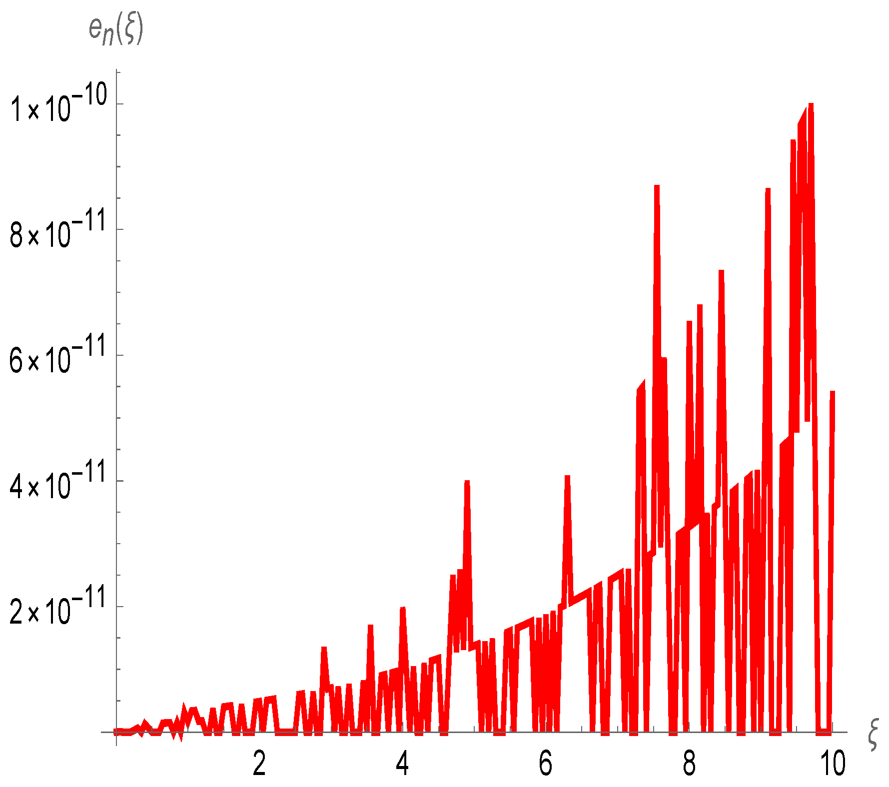
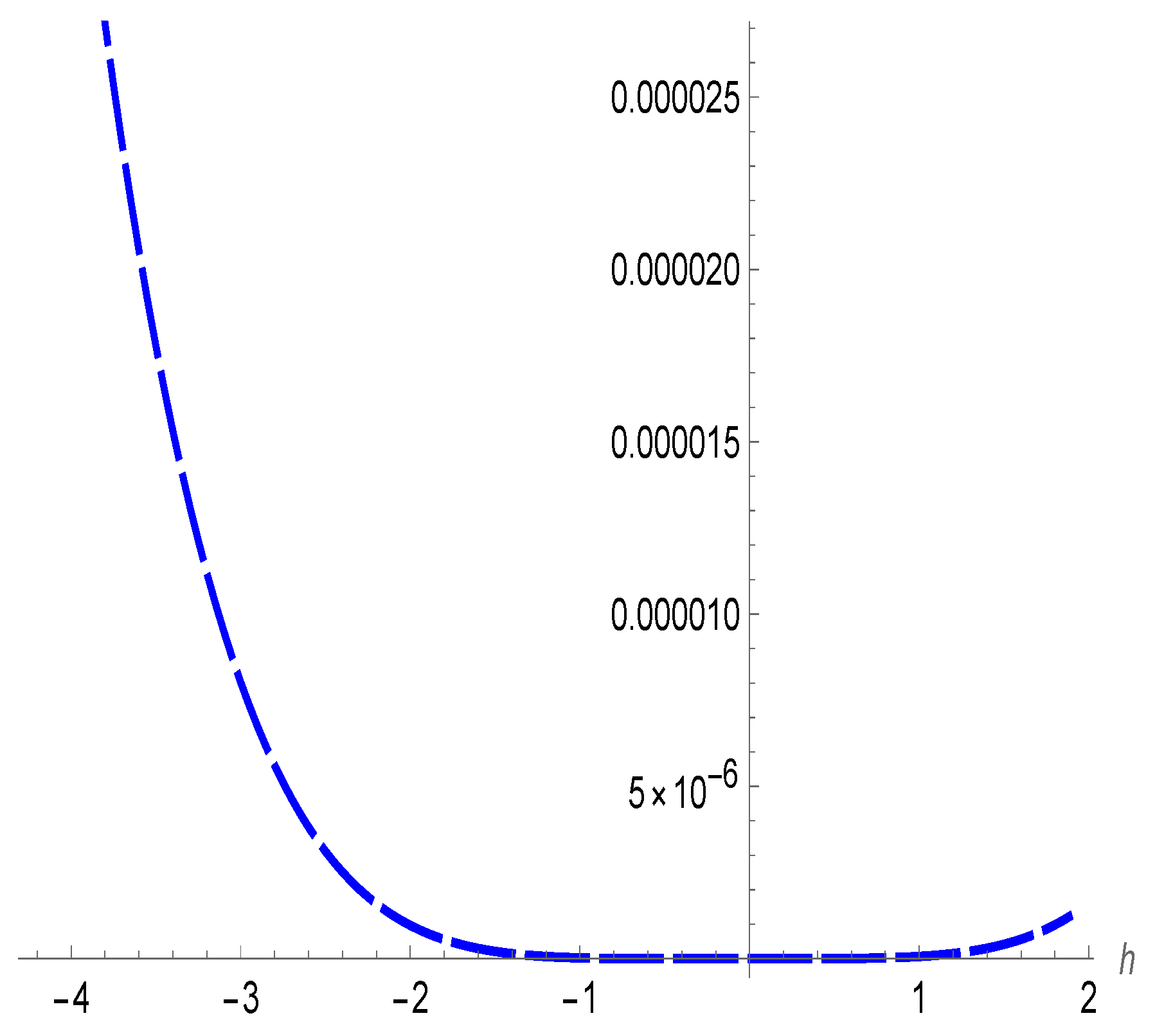
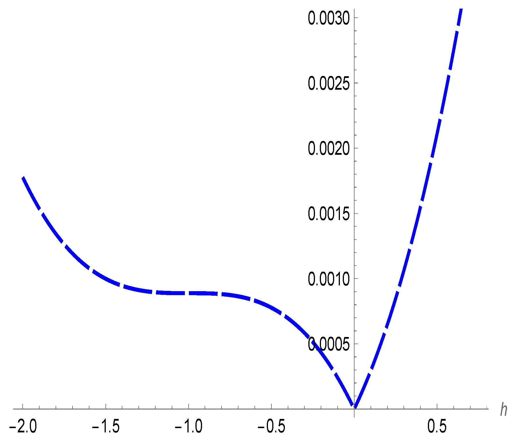
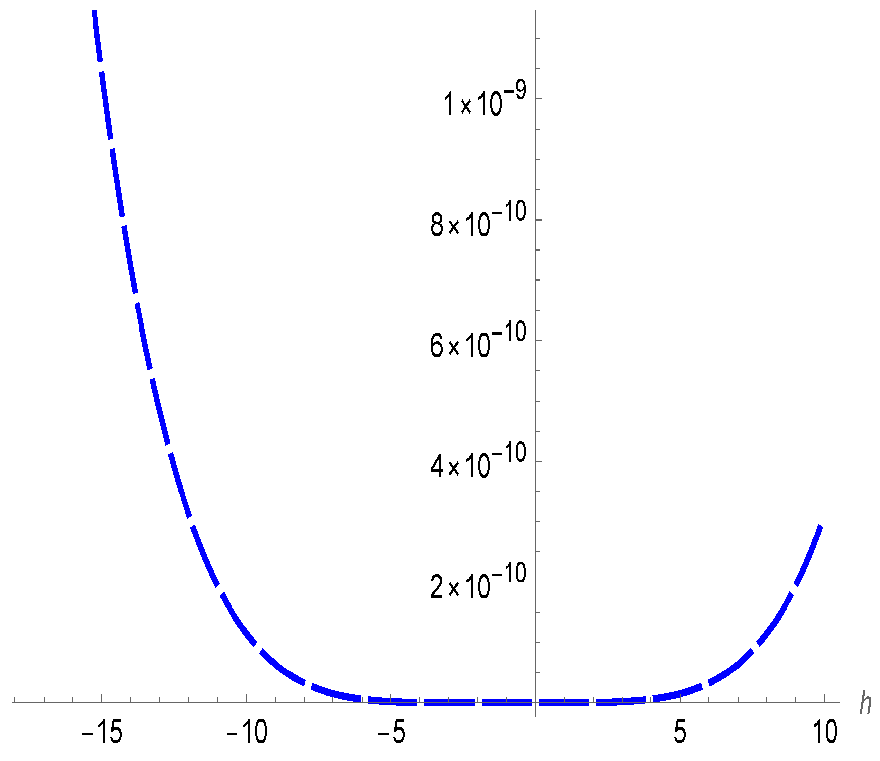
4. Numerical Results and Discussion

Example 1. 

Consider the following singular initial value problem [7]:

$$\left\{\begin{array}{c}{u}^{″}\left(\xi \right)+{\displaystyle \frac{2}{\xi }}{u}^{\prime }\left(\xi \right)+u^5\left(\xi \right)=0,\xi >0\hfill \\ u\left(0\right)=1,u^{\prime }\left(0\right)=0,\hfill \end{array}\right.$$

(44)

where the exact solution $u\left(\xi \right)={\displaystyle \frac{1}{\sqrt{\frac{{\xi }^2}{3}+1}}}$. By integrating Equation (44) two times and using the initial conditions, Equation (44) can be converted to the third-kind NV-IE as follows:

$$\xi u\left(\xi \right)=\xi -{\int }_0^{\xi }(\xi -\nu )\nu u^5\left(\nu \right)d\nu ,$$

(45)

In this example, comparing the approximate solution, which utilizes the HAM at $n=5$ and $h=0.01$ with the exact solution, the error behavior is shown in Figure 1. It illustrates that these parameters provide a good approximation for the solution and that $h=0.01$ is an optimal choice for convergence. Further, Figure 2 displays the behavior of maximum error $e_{max}\left(h\right)=\underset{i}{max}|u({\xi }_i,h)-u_n({\xi }_i,h)|\forall {\xi }_i\in [0,10]$, which indicates that the best valid region of h is $[-1.4,0.9]-\left\{0\right\}$.

Shiralashetti et al. [7] employed the Haar wavelet collocation method (HWCM) to derive a numerical solution for Equation (44). In contrast, our study utilized the HAM to solve Equation (45), demonstrating that our results achieve significantly higher accuracy compared to those presented in [7]. This enhanced precision is thoroughly examined and validated in

Table 1. Comparison of the maximum error $e_{max}\left(\xi \right)$ for the HAM and HWCM [7].

HAM	HWCM
$8\times {10}^{-10}$	$24\times {10}^{-6}$

, which provides a detailed comparison of the numerical outcomes. The superior accuracy of the HAM underscores its effectiveness and reliability in addressing the specific challenges posed by the equation, highlighting its advantages over the HWCM approach in this context.

Example 2. 

Consider the following nonlinear Lane Emden equation [10]:

$$\left\{\begin{array}{c}{u}^{″}\left(\xi \right)+{\displaystyle \frac{2}{\xi }}{u}^{\prime }\left(\xi \right)-6u\left(\xi \right)=4u\left(\xi \right)ln\left(u\left(\xi \right)\right),\xi >0\hfill \\ u\left(0\right)=1,u^{\prime }\left(0\right)=0,\hfill \end{array}\right.$$

(46)

where the exact solution $u\left(\xi \right)=e^{{\xi }^2}$. By integrating Equation (46) two times and using the initial conditions, Equation (46) can be converted to the third-kind NM-IDE as follows:

$$\xi u\left(\xi \right)=\xi +6{\int }_0^{\xi }(\xi -\nu )\nu u\left(\nu \right)d\nu +4{\int }_0^{\xi }(\xi -\nu )\nu u\left(\nu \right)ln\left(u\left(\nu \right)\right)d\nu ,$$

(47)

According to Figure 3, which uses the HAM to show the error behavior (in this case, at $n=5$ and $h=-0.05$), these parameters provide a good approximation for the solution, and $h=-0.05$ is the best choice for convergence. Moreover, Figure 4 displays the behavior of maximum error $e_{max}\left(h\right)\forall {\xi }_i\in [0,5]$ and shows that the best valid region of h is $[-0.4,0)$.

In [10], Geng et al. explored the numerical solution of Equation (46) by integrating the Replicating kernel Hilbert space approach (RKHSA) with the homotopy perturbation method (HPM). Building on this work, we applied the HAM to Equation (47) and achieved results far more accurate than those reported in [10]. This superior precision is clearly demonstrated in

Table 2. Comparison of the maximum error $e_{max}\left(\xi \right)$ for the HAM and RKHSA with HPM [10].

HAM	RKHSA with HPM
$1.2\times {10}^{-13}$	$2.16\times {10}^{-5}$

, which provides a comprehensive comparison of the numerical outcomes. The enhanced accuracy of our results underscores the effectiveness and robustness of the HAM in addressing the complexities of the equation, highlighting its advantages over the combined RKHSA and HPM approach used in previous studies.

Example 3. 

Consider the following Lienard equation [8]:

$$\left\{\begin{array}{c}{u}^{″}\left(\xi \right)+u\left(\xi \right)u^{\prime }\left(\xi \right)+u\left(\xi \right)+u^2\left(\xi \right)=f\left(\xi \right),\xi >0\hfill \\ u\left(0\right)=1,u^{\prime }\left(0\right)=0,\hfill \end{array}\right.$$

(48)

where $f\left(\xi \right)={cos}^2\xi -sin\xi cos\xi$, and the exact solution $u\left(\xi \right)=cos\left(\xi \right)$. By integrating Equation (48) two times and using the initial conditions, Equation (48) becomes

$$u\left(\xi \right)=H\left(\xi \right)-{\int }_0^{\xi }(\xi -\nu )u\left(\nu \right)d\nu -{\int }_0^{\xi }(\xi -\nu +{\displaystyle \frac{1}{2}})u^2\left(\nu \right)d\nu ,$$

(49)

The error behavior (in this case, employing the HAM at $n=3$ and $h=-0.02$) is shown in Figure 5. These parameters provide a good approximation for the solution, and $h=-0.02$ is the optimal choice for convergence. Further, Figure 6 displays the behavior of maximum error $e_{max}\left(h\right)\forall {\xi }_i\in [0,4]$, which indicates that the best valid region of h is $[-0.2,0)$.

A particular Schauder basis that is naturally related to the differential problem was used by Gámez et al. [8] to approximate the solution of Equation (48). We used the HAM to estimate the solution of Equation (49) in our study, and we showed that our results are more accurate than those found in [8].

Table 3. Comparison of the maximum error $e_{max}\left(\xi \right)$ for the HAM and SB [8].

HAM	SB
$9\times {10}^{-6}$	$5.89\times {10}^{-5}$

, which offers a thorough comparison of the numerical results, carefully verifies this improved precision. The higher accuracy of our findings demonstrates the efficacy and dependability of our methodology in handling the equation’s complexity and emphasizes its benefits over the Schauder basis method used in previous research.

Example 4. 

Consider the following Duffing equation [9]:

$$\left\{\begin{array}{c}{u}^{″}\left(\xi \right)+u^{\prime }\left(\xi \right)+\xi (1-\xi )u^3\left(\xi \right)=f\left(\xi \right),\hfill \\ u\left(0\right)=0,u^{\prime }\left(0\right)=\pi ,0\le \xi <1,\hfill \end{array}\right.$$

(50)

where $f\left(\xi \right)=(1-\xi )\xi {sin}^3\left(\pi \xi \right)-{\pi }^{2}sin\left(\pi \xi \right)+\pi cos\left(\pi \xi \right)$, and the exact solution $u\left(\xi \right)=sin\left(\pi \xi \right)$. By integrating Equation (50) two times and using the initial conditions, Equation (50) can be converted to

$$u\left(\xi \right)=H\left(\xi \right)+{\int }_0^{\xi }u\left(\nu \right)d\nu +{\displaystyle \frac{1}{2}}{\int }_0^{\xi }(\xi -\nu )\nu (1-\nu )u^3\left(\nu \right)d\nu ,$$

(51)

Using the HAM at $n=10$ and $h=-0.15$ in this example results in the error behavior seen in Figure 7. The ideal value for convergence is $h=-0.15$, and these parameters provide a decent approximation for the solution. Moreover, Figure 8 shows the behavior of maximum error $e_{max}\left(h\right)\forall {\xi }_i\in [0,10]$, which indicates that the best valid region of h is $[-4.9,4.3]-\left\{0\right\}$.

In [9], Chen et al. developed an approximate solution for Equation (50) by enhancing the reproducing kernel method (RKM). In our study, we applied the HAM to Equation (51) and demonstrated that our results surpass the accuracy of those reported in [9]. This significant improvement in precision is clearly illustrated in

Table 4. Comparison of the maximum error $e_{max}\left(\xi \right)$ for the HAM and RKM [9].

HAM	RKM
$6\times {10}^{-10}$	$1.4\times {10}^{-9}$

, which provides a detailed comparative analysis of the numerical results. The enhanced accuracy achieved through the HAM underscores its superior capability in addressing the intricacies of the equation, highlighting its effectiveness over the improved RKM approach utilized in prior research.

5. Conclusions

In this paper, we considered a novel strategy that is the conversion of traditional IVPs into NM-IDEs of the third kind. In addition, we discussed the existence and uniqueness of the solution using Picard’s method. Moreover, we presented the HAM to obtain the approximate solution. To demonstrate the reliability and accuracy of the proposed method and to depict the error behavior, illustrative examples were provided. In conclusion, converting IVPs to NM-IDEs and using the HAM offers significant computational advantages.

References

1. Brenan, K.E.; Campbell, S.L.; Petzold, L.R. Numerical Solution of Initial-Value Problems in Differential-Algebraic Equations; SIAM: Philadelphia, PA, USA, 1995. [Google Scholar]
2. Wanner, G.; Hairer, E. Solving Ordinary Differential Equations II; Springer: Berlin/Heidelberg, Germany, 1996; Volume 375. [Google Scholar]
3. Mickens, R.E. Truly Nonlinear Oscillations: Harmonic Balance, Parameter Expansions, Iteration, and Averaging Methods; World Scientific: Singapore, 2010. [Google Scholar]
4. Biazar, J.; Ghanbari, B. HAM solution of some initial value problems arising in heat radiation equations. J. King Saud Univ. Sci. 2012, 24, 161–165. [Google Scholar]
5. Mosa, G.A.; Abdou, M.A.; Rahby, A.S. Numerical solutions for nonlinear Volterra-Fredholm integral equations of the second kind with a phase lag. AIMS Math. 2021, 6, 8525–8543. [Google Scholar]
6. Rahby, A.S.; Abdou, M.A.; Mosa, G.A. On the solutions of the second kind nonlinear Volterra-Fredholm integral equations via homotopy analysis method. Int. J. Anal. Appl. 2022, 20, 35. [Google Scholar]
7. Shiralashetti, S.C.; Deshi, A.B.; Desai, P.B.M. Haar wavelet collocation method for the numerical solution of singular initial value problems. Ain Shams Eng. J. 2016, 7, 663–670. [Google Scholar]
8. Gámez, D.; Guillem, A.I.G.; Galán, M.R. Nonlinear initial-value problems and Schauder bases. Nonlinear Anal. Theory Methods Appl. 2005, 63, 97–105. [Google Scholar]
9. Chen, Z.; Jiang, W.; Du, H. A new reproducing kernel method for Duffing equations. Int. J. Comput. Math. 2021, 98, 2341–2354. [Google Scholar]
10. Geng, F.; Cui, M.; Zhang, B. Method for solving nonlinear initial value problems by combining homotopy perturbation and reproducing kernel Hilbert space methods. Nonlinear Anal. Real World Appl. 2010, 11, 637–644. [Google Scholar]
11. Abdulqader, A.J.; Abdulmaged, R.B.; Abdali, B.M. Numerical solution for solving nonlinear Volterra-Fredholm system by using iterative techniques. J. Interdiscip. Math. 2024, 27, 991–1000. [Google Scholar]
12. Mahdy, A.M.S.; Abdou, M.A.; Mohamed, D.S. Numerical solution, convergence and stability of error to solve quadratic mixed integral equation. J. Appl. Math. Comput. 2024, 70, 5887–5916. [Google Scholar] [CrossRef]
13. Alalyani, A.; Abdou, M.A.; Basseem, M. The orthogonal polynomials method using Gegenbauer polynomials to solve mixed integral equations with a Carleman kernel. AIMS Math. 2024, 9, 19240–19260. [Google Scholar]
14. Achar, S.D. Symmetric multistep Obrechkoff methods with zero phase-lag for periodic initial value problems of second order differential equations. Appl. Math. Comput. 2011, 218, 2237–2248. [Google Scholar]
15. Wang, B.; Liu, K.; Wu, X. A Filon-type asymptotic approach to solving highly oscillatory second-order initial value problems. J. Comput. Phys. 2013, 243, 210–223. [Google Scholar] [CrossRef]
16. Rahmanzadeh, M.; Cai, L.; White, R.E. A new method for solving initial value problems. Comput. Chem. Eng. 2013, 58, 33–39. [Google Scholar] [CrossRef]
17. Baccouch, M. A posteriori error estimates and adaptivity for the discontinuous Galerkin solutions of nonlinear second-order initial-value problems. Appl. Numer. Math. 2017, 121, 18–37. [Google Scholar] [CrossRef]
18. Baccouch, M. Superconvergence of the discontinuous Galerkin method for nonlinear second-order initial-value problems for ordinary differential equations. Appl. Numer. Math. 2017, 115, 160–179. [Google Scholar] [CrossRef]
19. Ramos, H.; Mehta, S.; Vigo-Aguiar, J. A unified approach for the development of k-step block Falkner-type methods for solving general second-order initial-value problems in ODEs. J. Comput. Appl. Math. 2017, 318, 550–564. [Google Scholar] [CrossRef]
20. Khalsaraei, M.M.; Shokri, A. An explicit six-step singularly P-stable Obrechkoff method for the numerical solution of second-order oscillatory initial value problems. Numer. Algorithms 2020, 84, 871–886. [Google Scholar] [CrossRef]
21. Yüzbaşı, S. A collocation method based on Bernstein polynomials to solve nonlinear Fredholm–Volterra integro-differential equations. Appl. Math. Comput. 2016, 273, 142–154. [Google Scholar] [CrossRef]
22. Alalyani, A.; Abdou, M.A.; Basseem, M. On a Solution of a Third Kind Mixed Integro-Differential Equation with Singular Kernel Using Orthogonal Polynomial Method. J. Appl. Math. 2023, 2023, 5163398. [Google Scholar] [CrossRef]
23. Hemeda, A.A. A friendly iterative technique for solving nonlinear integro-differential and systems of nonlinear integro-differential equations. Int. J. Comput. Methods 2018, 15, 1850016. [Google Scholar] [CrossRef]
24. Hamed, Y.S.; Amer, Y.A. Nonlinear saturation controller for vibration supersession of a nonlinear composite beam. J. Mech. Sci. Technol. 2014, 28, 2987–3002. [Google Scholar] [CrossRef]
25. Warminski, J.; Bochenski, M.; Jarzyna, W.; Filipek, P.; Augustyniak, M. Active suppression of nonlinear composite beam vibrations by selected control algorithms. Commun. Nonlinear Sci. Numer. Simul. 2011, 16, 2237–2248. [Google Scholar]
26. Warminski, J.; Cartmell, M.P.; Bochenski, M.; Ivanov, I. Analytical and experimental investigations of an autoparametric beam structure. J. Sound Vib. 2008, 315, 486–508. [Google Scholar] [CrossRef]
27. Liao, S. Homotopy analysis method: A new analytic method for nonlinear problems. Appl. Math. Mech. 1998, 19, 957–962. [Google Scholar]
28. Cherruault, Y. Convergence of Adomian’s method. Kybernetes 1989, 18, 31–38. [Google Scholar]
Figure 1. The behavior of the error at n = 5 ,   h = 0.01 employing HAM.
Axioms 14 00282 g001
Figure 2. The maximum error e m a x ( h ) behavior at n = 5 with corresponding h using HAM.
Axioms 14 00282 g002
Figure 3. The error behavior at n = 5 ,   h = 0.05 using HAM.
Axioms 14 00282 g003
Figure 4. The maximum error e m a x ( h ) behavior at n = 5 with corresponding h using HAM.
Axioms 14 00282 g004
Figure 5. The error behavior employing the HAM at n = 3 , h = 0.02 .
Axioms 14 00282 g005
Figure 6. The maximum error e m a x ( h ) behavior at n = 3 with corresponding h using HAM.
Axioms 14 00282 g006
Figure 7. The error behavior at n = 10 and h = 0.15 when utilizing HAM.
Axioms 14 00282 g007
Figure 8. The maximum error e m a x ( h ) behavior at n = 5 with corresponding h using HAM.
Axioms 14 00282 g008