Global Bifurcation in a General Leslie Type Predator–Prey System with Prey Taxis

Abstract

In this paper, the local and global structure of positive solutions for a general predator–prey model in a multi-dimension with ratio-dependent predator influence and prey taxis is investigated. By analyzing the corresponding characteristic equation, we first obtain the local stability conditions of the positive equilibrium caused by prey taxis. Secondly, taking the prey-taxis coefficient as a bifurcation parameter, we obtain the local structure of the positive solution by resorting to an abstract bifurcation theorem, and then extend the local solution branch to a global one. Finally, the local stability of such bifurcating positive solutions is discussed by the method of the perturbation of simple eigenvalues and spectrum theory. The results indicate that attractive prey taxis can stabilize positive equilibrium and inhibits the emergence of spatial patterns, while repulsive prey taxis can lead to Turing instability and induces the emergence of spatial patterns.

1. Introduction

Since the classical Lotka–Volterra model proposed by Lotka [1] and Volterra [2], predator–prey models have become one of the best-developed areas in ecology systems and have been widely studied. To better reflect the realistic phenomena and features of the ecosystem, the Lotka–Volterra model has been modified and improved in many forms [3,4,5,6]. In order to improve the random process, many researchers added spatial variables to the system, and the spatiotemporal dynamics of the diffusion predator–prey system have received widespread attention [7,8,9]. In fact, the spatiotemporal dynamics of the reaction–diffusion predator–prey system were affected not only by the random diffusion of predators and the prey, but also by the spatiotemporal variations of the predator’s velocity, which is often influenced by prey taxis. After the prey-taxis phenomenon was first observed by Kareiva and Odell [10] in the experiment, numerous diffusion systems with prey taxis have been studied to interpret the phenomenon of predator aggregation in high-prey-density areas [11,12,13]. It may be noted that the prey taxis yields complex spatiotemporal dynamics, such as periodic solutions, quasi-periodic solutions, or sphere-like surfaces of solutions [14,15,16].

It should be noted that many existing discussions [17,18,19] are focused on the Gause–Kolmogorov-type predator–prey model, there is little work on a general Leslie type predator–prey system with prey taxis. Therefore, we shall consider the following system with prey taxis

$$\begin{array}{c}\hfill \left\{\begin{array}{cc}{\displaystyle \frac{\partial u}{\partial t}}=d_1\Delta u+uf\left(u\right)-vg\left(u\right),\hfill & x\in \Omega ,t>0,\hfill \\ {\displaystyle \frac{\partial v}{\partial t}}=d_2\Delta v-\nabla (\chi v\nabla u)+vh\left({\displaystyle \frac{v}{u}}\right),\hfill & x\in \Omega ,t>0,\hfill \\ {\displaystyle \frac{\partial u}{\partial \nu }}={\displaystyle \frac{\partial v}{\partial \nu }}=0,\hfill & x\in \partial \Omega ,t>0,\hfill \\ u(x,0)=u_0\left(x\right)>0,v(x,0)=v_0\left(x\right)\ge 0,\hfill & x\in \Omega .\hfill \end{array}\right.\end{array}$$

(1)

where $\Omega$ is a bounded domain in ${\mathbb{R}}^n(n\ge 1)$ with a smooth boundary $\partial \Omega$ and outward unit normal vector $\nu$; $u=u(x,t)$ and $v=v(x,t)$ represent the densities of the prey and predator at time $t>0$ and position $x\in \Omega$, respectively; the Laplacian operator $\Delta$ denotes the random movement of two species; $d_1>0$ and $d_2>0$ are the diffusion coefficients for the prey and predator; the natural per capita growth function $f\left(u\right)$ describes the specific growth rate of the prey in the absence of predation; the function $g\left(u\right)$ represents the functional response of predators to the prey, and the function $h\left({\displaystyle \frac{v}{u}}\right)$ denotes the per capita growth function of the predator with prey-dependent carrying capacity. $-\nabla (\chi v\nabla u)$ represents the tendency of predators to move along the prey gradient direction, $\chi$ is the taxis coefficient of the predator, and the prey taxis is called attractive (repulsive) if $\chi >0(\chi <0)$. For more biological background information, readers can refer to [20,21].

For some specific forms of system (1), many excellent results have been obtained through qualitative or numerical analysis. For the case $d_1=d_2=\chi =0$, the system (1) has been considered by many authors [22,23,24]. Lindstrom [25] showed that the system may appear to have multiple equilibria and multiple limit cycles, as the half saturation of predators is low. By using Liapunov function and LaSalle’s invariance principle, the global asymptotic stability of the unique interior equilibrium was proved in [26]. Freedman and Mathsen [27] derived the criteria for persistence by transforming variables. Lan and Zhu [28] studied the phase portraits and Hopf bifurcation, and they proved that there is a unique stable limit cycle of the system by computing the Lyapunov number.

For the case $\chi =0$, the system (1) also has more interesting dynamical behavior, such as the existence and boundedness of positive solutions, the global stability of the interior equilibrium, bifurcation, and the stability of spatially nonhomogeneous steady-state solutions [29,30,31]. Du and Hsu [32] obtained the existence conditions of positive steady-state solutions, and proved that positive steady states with certain spatial patterns can appear for a suitable heterogeneous environment. The Turing instability of the equilibrium and the Hopf bifurcation were discussed in [33], and they also researched the stability of the bifurcating spatially homogeneous periodic solution. Qi and Zhu [34] obtained an improved condition for the global asymptotic stability of the unique positive equilibrium by using a novel comparison argument. For a general diffusive system, Zou and Guo [35] investigated the existence and boundedness conditions of positive steady-state solutions and also carried out the Hopf and steady-state bifurcation analyses.

Recently, when $\chi \ne 0$ in system (1), Wang et al. [36] considered the linearized stability of the positive equilibrium, and investigated the local existence and stability of nonconstant positive steady states through rigorous local bifurcation analysis in the 1D case. Zhang and Fu [37] discussed the structure of the set of the nonconstant steady states in detail for the Holling–Tanner predator–prey model. They found that attractive prey taxis can stabilize the homogeneous equilibrium even if diffusion-driven instability has occurred. By the asymptotic analysis and bifurcation theory, Qiu and Guo [38] obtained the local and global structure of nonconstant positive steady states of a modified Leslie–Gower model.

The main purpose of this paper is to find the nonconstant steady states of (1) by solving the following system

$$\begin{array}{c}\hfill \left\{\begin{array}{cc}{d}_1\Delta u+uf\left(u\right)-vg\left(u\right)=0,\hfill & x\in \Omega ,\hfill \\ d_2\Delta v-\nabla (\chi v\nabla u)+vh\left({\displaystyle \frac{v}{u}}\right)=0,\hfill & x\in \Omega ,\hfill \\ {\displaystyle \frac{\partial u}{\partial \nu }}={\displaystyle \frac{\partial v}{\partial \nu }}=0,\hfill & x\in \partial \Omega .\hfill \end{array}\right.\end{array}$$

(2)

In order to explore the steady-state bifurcation of system (2), we always assume that:

$\left(H1\right)$ $f\in C^1\left(\mathbb{R}\right)$, $f\left(0\right)>0$, there exists $K>0$ such that $f\left(K\right)=0$ and $f^{\prime }\left(u\right)<0$ for any $u>0$;

$\left(H2\right)$ $g\in C^1\left(\mathbb{R}\right)$, $g\left(0\right)=0$ and $g^{\prime }\left(u\right)>0$ for any $u>0$;

$\left(H3\right)$ $h\in C^1\left(\mathbb{R}\right)$, $h\left(0\right)>0$, there exists $\xi >0$ such that $h\left(\xi \right)=0$ and $h^{\prime }\left(s\right)<0$ for any $s>0$.

The remainder of this paper is organized as follows. In Section 2, we discuss the local linear stability of the unique positive equilibrium of system (1) by analyzing the characteristic equation. And, we also show that the pattern formation may arise only when $\chi <0$. In Section 3, the existence of nonconstant positive solutions is proved by an abstract bifurcation theorem. The linear stability of these bifurcating solutions for system (2) is considered in Section 4. In Section 5, the paper ends with a conclusion.

2. Stability of the Positive Equilibrium

According to the assumptions of $\left(H1\right),\left(H2\right),\left(H3\right)$, it is easy to see that system (1) has a boundary equilibrium $(K,0)$ and a unique positive equilibrium $(u^{\ast },v^{\ast })=(\tau ,\xi \tau )$, where $0<\tau <K$ is the unique one that satisfies $f\left(\tau \right)=\xi g\left(\tau \right)$.

Notations: $\alpha =f\left(\tau \right)+\tau f^{\prime }\left(\tau \right)-\xi \tau g^{\prime }\left(\tau \right),\beta =\xi h^{\prime }\left(\xi \right).$

By the assumptions, we know that $\alpha -f\left(\tau \right)=\tau f^{\prime }\left(\tau \right)-\xi \tau g^{\prime }\left(\tau \right)<0$ and $\beta <0$. In order to discuss the influence of prey taxis on the stability of the positive equilibrium, we assume the condition

$$\left(A0\right):\alpha +\beta <0$$

always holds to guarantee that the positive equilibrium $(u^{\ast },v^{\ast })$ is stable for the corresponding ordinary differential system of (1).

The linearization of the system (1) at the positive equilibrium $(u^{\ast },v^{\ast })$ is

$$U_t=D\Delta U+JU,$$

where

$$\begin{array}{c}\hfill U={(u,v)}^T,D=\left[\begin{array}{cc}{d}_1& 0\\ -\chi \xi \tau & d_2\end{array}\right]andJ=\left[\begin{array}{cc}\alpha & -g\left(\tau \right)\\ -\xi \beta & \beta \end{array}\right].\end{array}$$

Denote $0={\mu }_0<{\mu }_1<{\mu }_2<...$ to be the simple eigenvalues of $-\Delta$ on $\Omega$ subject to the homogeneous Neumann boundary condition and let the corresponding normalized eigenfunction be ${\varphi }_k\left(x\right)$.

Then, the characteristic equations corresponding to the positive equilibrium $(u^{\ast },v^{\ast })$ are

$${\Gamma }_k\left(\chi \right)={\lambda }^2-T_k\left(\chi \right)\lambda +D_k\left(\chi \right)=0,k\in {\mathbb{Z}}^{+}\bigcup \left\{0\right\},$$

(3)

where

$$T_k\left(\chi \right)=-(d_1+d_2){\mu }_k+\alpha +\beta ,$$

$$D_k\left(\chi \right)=d_1{d}_2{\mu }_k^2+(\chi \xi \tau g\left(\tau \right)-\alpha d_2-\beta d_1){\mu }_k+\beta (\alpha -f\left(\tau \right)).$$

Clearly, $T_k\left(\chi \right)<0$ for arbitrarily $k\in {\mathbb{Z}}^{+}\bigcup \left\{0\right\}$ and $D_0\left(\chi \right)>0$ by $\left(A0\right)$. Thus, in order to investigate the instability of the positive equilibrium $(u^{\ast },v^{\ast })$, we need to find a $k\in {\mathbb{Z}}^{+}$ such that $D_k\left(\chi \right)=D_k\left(0\right)+\chi \xi \tau g\left(\tau \right){\mu }_k<0$. Let

$$P\left({\mu }_k\right)={\displaystyle \frac{D_k\left(0\right)}{\xi \tau g\left(\tau \right){\mu }_k}}={\displaystyle \frac{d_1{d}_2{\mu }_k^2-(\alpha d_2+\beta d_1){\mu }_k+\beta (\alpha -f\left(\tau \right))}{\xi \tau g\left(\tau \right){\mu }_k}}$$

and

$$Q\left(x\right)={\displaystyle \frac{d_1{d}_2{x}^2-(\alpha d_2+\beta d_1)x+\beta (\alpha -f\left(\tau \right))}{\xi \tau g\left(\tau \right)x}},x>0.$$

Through calculation, we determine that $Q\left(x\right)$ is decreasing on $(0,x_0)$ and increasing on $(x_0,+\infty )$, where $x_0=\sqrt{{\displaystyle \frac{\beta (\alpha -f(\tau \left)\right)}{d_1{d}_2}}}$, and there exists a constant $k_0\in {\mathbb{Z}}^{+}$ such that ${\mu }_{k_0}\le x_0<{\mu }_{k_0+1}$. Set

$$\begin{array}{c}\hfill {\chi }_{max}=-min\{P\left({\mu }_{k_0}\right),P\left({\mu }_{k_0+1}\right)\}=-\underset{k\in {\mathbb{Z}}^{+}}{min}{\displaystyle \frac{D_k\left(0\right)}{\xi \tau g\left(\tau \right){\mu }_k}}.\end{array}$$

(4)

Thereby, there is at least some $k\in {\mathbb{Z}}^{+}$ such that $D_k\left(\chi \right)<0$ when $\chi <{\chi }_{max}$. This leads to the following theorem.

Theorem 1.

Assume $\left(A0\right)$ holds; then, the positive equilibrium $(u^{\ast },v^{\ast })$ of system (1) is stable for $\chi >{\chi }_{max}$ and it is unstable if $\chi <{\chi }_{max}$.

Remark 1.

It is easy to check that if $D_k\left(0\right)>0$ for all $k\in {\mathbb{Z}}^{+}$, then ${\chi }_{max}<0$ and the positive equilibrium $(u^{\ast },v^{\ast })$ is stable for the system (1) without prey taxis. By Theorem 1, this implies that only repulsive prey taxis can lead to Turing instability and induces the emergence of spatial patterns. However, if there exists some $k\in {\mathbb{Z}}^{+}$ such that $D_k\left(0\right)<0$, then ${\chi }_{max}>0$ and the positive equilibrium $(u^{\ast },v^{\ast })$ are instable for the system (1) without prey taxis. From Theorem 1, which shows that attractive prey taxis can stabilize positive equilibrium and inhibits the emergence of spatial patterns. These are all different from indirect prey taxis; readers can refer to Theorem $2.1$ in [39].

Example 1.

To verify our above analysis, we investigate the diffusive Leslie–Gower predator–prey model with herd behavior and prey taxis in 1D spatial domain $\Omega =(0,10\pi )$. That is, $f\left(u\right)=1-u,g\left(u\right)={\displaystyle \frac{\sqrt{u}}{1+a\sqrt{u}}}$ and $h\left({\displaystyle \frac{v}{u}}\right)=b-{\displaystyle \frac{v}{ru}}$.

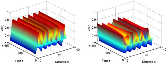
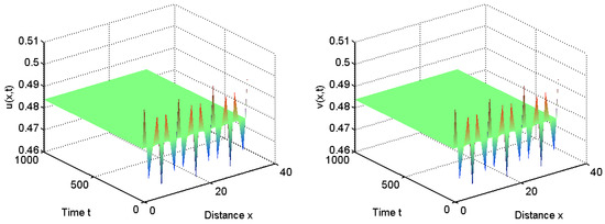
Let us first take $d_1=0.1,d_2=4,a=0.5,b=1,r=1$; we have that $D_k\left(0\right)>0$ for all $k\in {\mathbb{Z}}^{+}$ and ${\chi }_{max}=-7.124$. From Theorem 1, the positive equilibrium $(u^{\ast },v^{\ast })=(0.4839,0.4839)$ is unstable for $\chi =-10<{\chi }_{max}$ and it is stable for $\chi =15>{\chi }_{max}$; see Figure 1 and Figure 2.

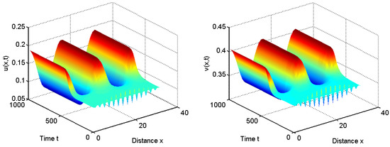
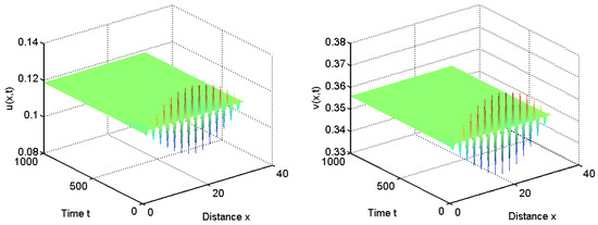
When we choose $d_1=1,d_2=40,a=0.5,b=2,r=1.5$, we have $D_k\left(0\right)<0$ for all $k=3,4,5$ and ${\chi }_{max}=28.0998$. From Theorem 1, the positive equilibrium $(u^{\ast },v^{\ast })=(0.1186,0.3558)$ is stable for $\chi =30>{\chi }_{max}$ and it is unstable for $\chi =15<{\chi }_{max}$; see Figure 3 and Figure 4.

3. Global Bifurcation

From the ecological viewpoint, a nonconstant positive solution corresponds to the coexistence steady state of prey and predator. Thus, the purpose of this section is to seek the nonconstant positive solutions of system (2) by an abstract bifurcation theorem. To discuss the bifurcation analysis of system (2), it is necessary to give a priori bound for any positive solutions of system (2).

Lemma 1.

Let $(u,v)$ be a positive solution of system (2). Then, $u,v\in C^{1,\varrho }\left(\overline{\Omega }\right)$ for all $\varrho \in (0,1)$ and

$$C\le u\le K,\xi C{e}^{-{\displaystyle \frac{2\left|\chi \right|K}{d_2}}}\le v\le \xi K{e}^{{\displaystyle \frac{2\left|\chi \right|K}{d_2}}}forallx\in \overline{\Omega },$$

where C is a positive constant.

Proof. 

By the first equation of system (2) and the maximum principle, we ensure that any positive solutions of system (2) satisfy $u\left(x\right)\le K$. And then, due to the Harnack inequality, there exists a positive constant $C^{\ast }$ such that $\underset{x\in \overline{\Omega }}{max}u\left(x\right)\le C^{\ast }\underset{x\in \overline{\Omega }}{min}u\left(x\right)$. Hence, there exists a positive constant C such that $C\le u\left(x\right)\le K$ for all $x\in \overline{\Omega }$.

Let $w=v{e}^{-{\displaystyle \frac{\chi }{d_2}}u}$; then, the second equation of system (2) becomes

$$d_2\nabla (e^{{\displaystyle \frac{\chi }{d_2}}u}\nabla w)+e^{{\displaystyle \frac{\chi }{d_2}}u}wh({\displaystyle \frac{e^{\frac{\chi }{d_2}u}w}{u}})=0.$$

Suppose that $x_0\in \overline{\Omega }$ is a maximum point of w; that is, $w\left(x_0\right)=\underset{x\in \overline{\Omega }}{max}w\left(x\right)$. In view of the boundedness of u and the maximum principle, we obtain

$$w\le w\left(x_0\right)\le \xi u\left(x_0\right)e^{-{\displaystyle \frac{\chi }{d_2}}u\left(x_0\right)}\le \xi K{e}^{{\displaystyle \frac{\left|\chi \right|K}{d_2}}}.$$

Thus, $v=w{e}^{{\displaystyle \frac{\chi }{d_2}}u}\le w{e}^{{\displaystyle \frac{\left|\chi \right|}{d_2}}K}\le \xi K{e}^{{\displaystyle \frac{2\left|\chi \right|K}{d_2}}}$. Similarly, let $x_1\in \overline{\Omega }$ be a point such that $w\left(x_1\right)=\underset{x\in \overline{\Omega }}{min}w\left(x\right)$, then

$$w\ge w\left(x_1\right)\ge \xi u\left(x_1\right)e^{-{\displaystyle \frac{\chi }{d_2}}u\left(x_1\right)}\ge \xi C{e}^{-{\displaystyle \frac{\left|\chi \right|K}{d_2}}}.$$

Hence, $v=w{e}^{{\displaystyle \frac{\chi }{d_2}}u}\ge w{e}^{{\displaystyle \frac{-\left|\chi \right|K}{d_2}}}\ge \xi C{e}^{-{\displaystyle \frac{2\left|\chi \right|K}{d_2}}}$.

Next, we shall show that $u,v\in C^{1,\varrho }\left(\overline{\Omega }\right)$ for all $\varrho \in (0,1)$. Since the first equation of system (2) and $u,v\in L^{\infty }(\Omega )$, we have $u\in W^{2,p}(\Omega )$ for any $p<\infty$ by standard elliptic regularity theory. Then, it follows from Sobolev embedding theorem that $W^{2,p}(\Omega )\hookrightarrow C^{1,\varrho }\left(\overline{\Omega }\right)$. Thus, $u\in C^{1,\varrho }\left(\overline{\Omega }\right)$ for $\varrho \in (0,1)$. Then, we rewrite the second equation of system (2) as follows

$$-d_2\Delta v+\chi \nabla v\nabla u=vh\left({\displaystyle \frac{v}{u}}\right)+{\displaystyle \frac{\chi }{d_1}}v(uf\left(u\right)-vg\left(u\right)).$$

Based on $C\le u\le K$ and $u\in W^{2,p}(\Omega )$, one obtains $v\in W^{2,p}(\Omega )$ for any $p<\infty$ from elliptic regularity theory. And, together with the Sobolev embedding theorem, we gain $v\in C^{1,\varrho }\left(\overline{\Omega }\right)$ for all $\varrho \in (0,1)$. Therefore, the proof is completed. □

In the following, we shall take the prey-taxis sensitivity coefficient $\chi$ as the bifurcation parameter; a branch of nonconstant stationary solutions is established by the Crandall–Rabinowitz’ss bifurcation theorem [40] and its user-friendly version given by Shi and Wang in [41]. The structure of positive solutions in the vicinity of $(u^{\ast },v^{\ast })$ is presented in detail by the local bifurcation theory, and then we extend the local curves by applying global bifurcation theory. To this end, we define

$$\begin{array}{cc}\hfill \mathcal{X}& =\{(u,v)\in W^{2,p}(\Omega )\times W^{2,p}(\Omega ):{\displaystyle \frac{\partial u}{\partial \nu }}={\displaystyle \frac{\partial v}{\partial \nu }}=0,on\partial \Omega \},\hfill \\ \hfill \mathcal{W}& =\{(\chi ,u,v)\in \mathbb{R}\times \mathcal{X}:u+u^{\ast }>0,v+v^{\ast }>0\},\hfill \\ \hfill \mathcal{Y}& =L^p(\Omega )\times L^p(\Omega )(p>n),\hfill \\ \hfill \mathcal{Z}& =\{(u,v)\in \mathcal{X}:{\int }_{\Omega }[u+{\displaystyle \frac{\alpha -d_1{\mu }_k}{g\left(\tau \right)}}v]{\varphi }_{k}dx=0\}.\hfill \end{array}$$

Let $\widehat{u}=u-u^{\ast },\widehat{v}=v-v^{\ast }$, and rewrite $\widehat{u},\widehat{v}$ back to $u,v$; system (2) becomes

$$\begin{array}{c}\hfill \left\{\begin{array}{cc}\mathcal{F}(\chi ,u,v)=0,\hfill & x\in \Omega ,\hfill \\ {\displaystyle \frac{\partial u}{\partial \nu }}={\displaystyle \frac{\partial v}{\partial \nu }}=0,\hfill & x\in \partial \Omega ,\hfill \end{array}\right.\end{array}$$

where

$$\begin{array}{c}\hfill \mathcal{F}(\chi ,u,v)=\left(\begin{array}{c}{d}_1\Delta u+(u+u^{\ast })f(u+u^{\ast })-(v+v^{\ast })g(u+u^{\ast })\\ d_2\Delta v-\nabla (\chi (v+v^{\ast })\nabla (u+u^{\ast }))+(v+v^{\ast })h\left({\displaystyle \frac{v+v^{\ast }}{u+u^{\ast }}}\right)\end{array}\right).\end{array}$$

Theorem 2.

Assume $\left(A0\right)$ holds. For each, $k\in {\mathbb{Z}}^{+}$ is fixed if

$$\chi ={\chi }_0\left(k\right)and{d}_1{d}_2{\mu }_j{\mu }_k\ne \beta (\alpha -f\left(\tau \right))),$$

where ${\chi }_0\left(k\right)=-{\displaystyle \frac{d_1{d}_2{\mu }_k^2-(\beta d_1+\alpha d_2){\mu }_k+\beta (\alpha -f\left(\tau \right))}{\xi \tau g\left(\tau \right){\mu }_k}}$ and $j\in {\mathbb{Z}}^{+}$, then a branch of nonconstant positive solution of system (2) bifurcates from the positive equilibrium $(u^{\ast },v^{\ast })$, and the bifurcating branch near the bifurcation point $({\chi }_0\left(k\right),u^{\ast },v^{\ast })$ can be parameterized as

$$\begin{array}{c}\hfill \chi \left(ϵ\right)={\chi }_0\left(k\right)+O\left(ϵ\right),(u_k(x,ϵ),v_k(x,ϵ))=(u^{\ast },v^{\ast })+ϵ(1,{\displaystyle \frac{\alpha -d_1{\mu }_k}{g\left(\tau \right)}}){\varphi }_k\left(x\right)+{ϵ}^2({\tilde{u}}_k(x,ϵ),{\tilde{v}}_k(x,ϵ)),\end{array}$$

with $({\tilde{u}}_k(x,ϵ),{\tilde{v}}_k(x,ϵ))\in \mathcal{Z}$ and $\left|ϵ\right|$ sufficiently small. Moreover, the bifurcating branch is part of a connected component ${\mathcal{C}}_0$ of the set $\overline{\mathcal{S}}$, where

$$\mathcal{S}=\left\{(\chi ,u,v)\right|(\chi ,u-u^{\ast },v-v^{\ast })\in \mathcal{W},\mathcal{F}(\chi ,u-u^{\ast },v-v^{\ast })=0,(u,v)\ne (u^{\ast },v^{\ast })\},$$

and ${\mathcal{C}}_0$ extends to infinity in χ as ${\mu }_k\ne {\displaystyle \frac{h\left(0\right)}{d_2}}$.

Proof. 

By direct computation, the Fr$\stackrel{’}{e}$chet derivative of $\mathcal{F}$ is given by

$$\begin{array}{cc}\hfill & {\mathcal{F}}_{(u,v)}(\chi ,u,v){(\phi ,\psi )}^T=\hfill \\ \hfill & \left(\begin{array}{c}{d}_1\Delta \phi +{\mathcal{G}}_1(\phi ,\psi )\\ d_2\Delta \psi -\chi \nabla [(v+v^{\ast })\nabla \phi +\psi \nabla (u+u^{\ast })]+{\mathcal{G}}_2(\phi ,\psi )\end{array}\right),\hfill \end{array}$$

(5)

where ${\mathcal{G}}_1(\phi ,\psi )=[f(u+u^{\ast })+(u+u^{\ast })f^{\prime }(u+u^{\ast })-(v+v^{\ast })g^{\prime }(u+u^{\ast })]\phi -g(u+u^{\ast })\psi$ and ${\mathcal{G}}_2(\phi ,\psi )=-{\displaystyle \frac{{(v+v^{\ast })}^2}{{(u+u^{\ast })}^2}}{h}^{\prime }\left({\displaystyle \frac{v+v^{\ast }}{u+u^{\ast }}}\right)\phi +[h\left({\displaystyle \frac{v+v^{\ast }}{u+u^{\ast }}}\right)+{\displaystyle \frac{v+v^{\ast }}{u+u^{\ast }}}{h}^{\prime }\left({\displaystyle \frac{v+v^{\ast }}{u+u^{\ast }}}\right)]\psi$. It is easy to verify that ${\mathcal{F}}_{(u,v)}(\chi ,u,v)$ is continuous and differentiable with respect to $\chi ,u,v$ in $\mathcal{W}$.

When defining $w={(\phi ,\psi )}^T$, (5) can be rewritten as

$$\begin{array}{c}\hfill {\mathcal{F}}_{(u,v)}(\chi ,u,v)w={\mathcal{L}}_0\Delta w+{\mathcal{F}}_1(\chi ,w,\nabla w),\end{array}$$

where

$$\begin{array}{ccc}\hfill {\mathcal{L}}_0& =\left[\begin{array}{cc}{d}_1& 0\\ -\chi (v+v^{\ast })& d_2\end{array}\right]and{\mathcal{F}}_1(\chi ,w,\nabla w)\hfill & \hfill =\left(\begin{array}{c}{\mathcal{G}}_1(\phi ,\psi )\\ -\chi \nabla v\nabla \phi -\chi \nabla (\psi \nabla u)+{\mathcal{G}}_2(\phi ,\psi )\end{array}\right).\end{array}$$

Clearly, $Trace\left({\mathcal{L}}_0\right)>0$ and $Det\left({\mathcal{L}}_0\right)>0$. Thus, from Corollary 2.11 of [41], ${\mathcal{F}}_{(u,v)}(\chi ,u,v)$ is the Fredholm operator with zero index.

To find the potential bifurcation point, we should show that the implicit function theorem fails on $\mathcal{F}$ under some values of $\chi$. This means that there exists a nontrivial solution for ${\mathcal{F}}_{(u,v)}(\chi ,0,0){(\phi ,\psi )}^T=0$; that is

$$\begin{array}{c}\hfill \left\{\begin{array}{cc}{d}_1\Delta \phi +\alpha \phi -g\left(\tau \right)\psi =0,\hfill & x\in \Omega ,\hfill \\ d_2\Delta \psi -\chi \xi \tau \Delta \phi -\xi \beta \phi +\beta \psi =0,\hfill & x\in \Omega ,\hfill \\ {\displaystyle \frac{\partial \phi }{\partial \nu }}={\displaystyle \frac{\partial \psi }{\partial \nu }}=0,\hfill & x\in \partial \Omega .\hfill \end{array}\right.\end{array}$$

(6)

In fact, any pair of function $(\phi ,\psi )\in \mathcal{X}$ can be expanded as follows

$$\begin{array}{c}\hfill \left(\begin{array}{c}\phi \left(x\right)\\ \psi \left(x\right)\end{array}\right)=\sum _{k=0}^{\infty }\left(\begin{array}{c}{a}_k\\ b_k\end{array}\right){\varphi }_k\left(x\right).\end{array}$$

(7)

If $(\phi ,\psi )\ne (0,0)$, then there is at least one of $(a_k,b_k)\ne (0,0)$. Thus, substituting the formula (7) into system (6), and multiplying the system (6) by ${\varphi }_k\left(x\right)$ and integrating over $\Omega$, together with ${\varphi }_k\left(x\right)$ as the normalized orthogonal eigenfunction, we obtain the following matrix equation

$$\begin{array}{c}\hfill \left[\begin{array}{cc}-d_1{\mu }_k+\alpha & -g\left(\tau \right)\\ \chi \xi \tau {\mu }_k-\xi \beta & -d_2{\mu }_k+\beta \end{array}\right]\left(\begin{array}{c}{a}_k\\ b_k\end{array}\right)=\left(\begin{array}{c}0\\ 0\end{array}\right).\end{array}$$

Note that $k=0$ can be easily ruled out. Hence, for $k\in {\mathbb{Z}}^{+}$, system (6) has nontrivial solutions equivalent to

$$\begin{array}{c}\hfill \left|\begin{array}{cc}-d_1{\mu }_k+\alpha & -g\left(\tau \right)\\ \chi \xi \tau {\mu }_k-\xi \beta & -d_2{\mu }_k+\beta \end{array}\right|=0.\end{array}$$

(8)

According to $f\left(\tau \right)=\xi g\left(\tau \right)$, we have

$$\begin{array}{c}\hfill \chi ={\chi }_0\left(k\right)=-{\displaystyle \frac{d_1{d}_2{\mu }_k^2-(\alpha d_2+\beta d_1){\mu }_k+\beta (\alpha -f\left(\tau \right))}{\xi \tau g\left(\tau \right){\mu }_k}}.\end{array}$$

In addition, in order to apply the bifurcation theory of a simple eigenvalue, we take $\chi ={\chi }_0\left(k\right)$, and multiply ${\displaystyle \frac{{\chi }_0\left(k\right)\xi \tau }{d_1}}$ to the first equation of system (6), then add it to the second equation; we obtain

$$\begin{array}{c}\hfill \left\{\begin{array}{cc}\Delta w+Aw=0,\hfill & x\in \Omega ,\hfill \\ {\displaystyle \frac{\partial w}{\partial \nu }}=0,\hfill & x\in \partial \Omega ,\hfill \end{array}\right.\end{array}$$

(9)

where

$$\begin{array}{c}\hfill A=\left[\begin{array}{cc}{\displaystyle \frac{\alpha }{d_1}}& -{\displaystyle \frac{g\left(\tau \right)}{d_1}}\\ {\displaystyle \frac{{\chi }_0\left(k\right)\xi \tau \alpha -d_1\xi \beta }{d_1{d}_2}}& -{\displaystyle \frac{{\chi }_0\left(k\right)\xi \tau g\left(\tau \right)-d_1\beta }{d_1{d}_2}}\end{array}\right].\end{array}$$

To consider the eigenvalues of the matrix A, we should find a value $\lambda$ such that

$$\begin{array}{c}\hfill \left|\begin{array}{cc}{\displaystyle \frac{\alpha }{d_1}}-\lambda & -{\displaystyle \frac{g\left(\tau \right)}{d_1}}\\ {\displaystyle \frac{{\chi }_0\left(k\right)\xi \tau \alpha -d_1\xi \beta }{d_1{d}_2}}& -{\displaystyle \frac{{\chi }_0\left(k\right)\xi \tau g\left(\tau \right)-d_1\beta }{d_1{d}_2}}-\lambda \end{array}\right|=0.\end{array}$$

After calculations, we obtain $Det\left(A\right)={\displaystyle \frac{\beta (\alpha -f(\tau \left)\right)}{d_1{d}_2}}>0$. And, from Equation (8), it is easy to check that ${\lambda }_1={\mu }_k$ is one of eigenvalues of A. So, another eigenvalue of A is ${\lambda }_2={\displaystyle \frac{\beta (\alpha -f(\tau \left)\right)}{d_1{d}_2{\mu }_k}}$. Thus, if ${\mu }_k\ne {\displaystyle \frac{\beta (\alpha -f(\tau \left)\right)}{d_1{d}_2{\mu }_k}}$, then the matrix A has two different positive real eigenvalues.

On the other hand, by reversible transformation, system (9) is equivalent to the following system

$$\begin{array}{c}\hfill \left\{\begin{array}{cc}\Delta \xi +B\xi =0,\hfill & x\in \Omega ,\hfill \\ {\displaystyle \frac{\partial \xi }{\partial \nu }}=0,\hfill & x\in \partial \Omega ,\hfill \end{array}\right.\end{array}$$

where $\xi ={({\xi }_1,{\xi }_2)}^T\in \mathcal{X}$ and $B=\left[\begin{array}{cc}{\lambda }_1& 0\\ 0& {\lambda }_2\end{array}\right].$ Hence, if ${\lambda }_2$ is not an eigenvalue of $-\Delta$ on $\Omega$ subject to the homogeneous Neumann boundary condition, i.e.,

$$d_1{d}_2{\mu }_j{\mu }_k\ne \beta (\alpha -f\left(\tau \right)))foranyj\in {\mathbb{Z}}^{+},$$

we have ${\xi }_1=c{\varphi }_k\left(x\right)$ and ${\xi }_2=0$, where c is a constant. Since the transformation is reversible, we obtain $\phi =c_1{\varphi }_k\left(x\right)$ and $\psi =c_2{\varphi }_k\left(x\right)$, where $c_1$ and $c_2$ are constants. By computing, we have

$$ker\left({\mathcal{F}}_{(u,v)}({\chi }_0\left(k\right),0,0)\right)=span\left\{{(1,{\displaystyle \frac{\alpha -d_1{\mu }_k}{g\left(\tau \right)}})}^T{\varphi }_k\left(x\right)\right\}.$$

Therefore, $dimker\left({\mathcal{F}}_{(u,v)}({\chi }_0\left(k\right),0,0)\right)=1$. Because we have proved that ${\mathcal{F}}_{(u,v)}(\chi ,u,v)$ is the Fredholm operator of index 0, it follows that $codimR\left({\mathcal{F}}_{(u,v)}({\chi }_0\left(k\right),0,0)\right)=1$.

Finally, we also need to prove the transversality condition ${\mathcal{F}}_{\chi (u,v)}({\chi }_0\left(k\right),0,0)w_0\notin R\left({\mathcal{F}}_{(u,v)}({\chi }_0\left(k\right),0,0)\right)$ holds, where

$$\begin{array}{c}\hfill w_0={(1,{\displaystyle \frac{\alpha -d_1{\mu }_k}{g\left(\tau \right)}})}^T{\varphi }_k\left(x\right).\end{array}$$

(10)

By (5) we have

$$\begin{array}{c}\hfill {\mathcal{F}}_{\chi (u,v)}(\chi ,u,v){(\phi ,\psi )}^T=\left(\begin{array}{c}0\\ -\nabla [(v+v^{\ast })\nabla \phi +\psi \nabla (u+u^{\ast })]\end{array}\right),\end{array}$$

(11)

is continuous, which yields

$$\begin{array}{c}\hfill {\mathcal{F}}_{\chi (u,v)}({\chi }_0\left(k\right),0,0)w_0=\left(\begin{array}{c}0\\ \xi \tau {\mu }_k\end{array}\right){\varphi }_k\left(x\right).\end{array}$$

Suppose that ${\mathcal{F}}_{\chi (u,v)}({\chi }_0\left(k\right),0,0)w_0\in R\left({\mathcal{F}}_{(u,v)}({\chi }_0\left(k\right),0,0)\right),$ then there exist a nontrivial solution $(\phi ,\psi )$, such that

$${\mathcal{F}}_{(u,v)}({\chi }_0\left(k\right),0,0)(\phi ,\psi )={\mathcal{F}}_{\chi (u,v)}({\chi }_0\left(k\right),0,0)w_0,$$

that is

$$\begin{array}{c}\hfill \left\{\begin{array}{cc}{d}_1\Delta \phi +\alpha \phi -g\left(\tau \right)\psi =0,\hfill & x\in \Omega ,\hfill \\ d_2\Delta \psi -{\chi }_0\left(k\right)\xi \tau \Delta \phi -\xi \beta \phi +\beta \psi =\xi \tau {\mu }_k{\varphi }_k,\hfill & x\in \Omega ,\hfill \\ {\displaystyle \frac{\partial \phi }{\partial \nu }}={\displaystyle \frac{\partial \psi }{\partial \nu }}=0,\hfill & x\in \partial \Omega .\hfill \end{array}\right.\end{array}$$

(12)

Note that ${\int }_{\Omega }{\varphi }_k^{2}dx=1$. Multiplying the first two equations in system (12) by ${\varphi }_k\left(x\right)$ and then integrating them over $\Omega$ by parts, we have

$$\begin{array}{c}\hfill \left[\begin{array}{cc}-d_1{\mu }_k+\alpha & -g\left(\tau \right)\\ {\chi }_0\left(k\right)\xi \tau {\mu }_k-\xi \beta & -d_2{\mu }_k+\beta \end{array}\right]\left(\begin{array}{c}{\int }_{\Omega }\phi {\varphi }_{k}dx\\ {\int }_{\Omega }\psi {\varphi }_{k}dx\end{array}\right)=\left(\begin{array}{c}0\\ \xi \tau {\mu }_k\end{array}\right).\end{array}$$

(13)

However, (13) is impossible because the determinant of the coefficient matrix on the left hand of (13) is zero by (8). So we obtain the contradiction, and it follows that ${\mathcal{F}}_{\chi (u,v)}({\chi }_0\left(k\right),0,0)$, $w_0\notin R\left({\mathcal{F}}_{(u,v)}({\chi }_0\left(k\right),0,0)\right).$

Thus, the local structure of nonconstant positive solutions near $(u^{\ast },v^{\ast })$ can be obtained by Crandall and Rabinowitz in Theorem 1.7 in [40]. Then, we extend the local solution branch to be a global one. According to the abstract global bifurcation theory of Shi and Wang [41], we know that ${\mathcal{C}}_0$ must fulfill one of the following:

$\left(i\right)$ ${\mathcal{C}}_0$ is unbounded in $\mathbb{R}\times \mathcal{X}$;

$\left(ii\right)$ ${\mathcal{C}}_0$ contains a point $({\chi }^{\ast },u^{\ast },v^{\ast })$ with ${\chi }^{\ast }\ne {\chi }_0\left(k\right)$;

$\left(iii\right)$ ${\mathcal{C}}_0$ contains a point where $(\chi ,u-u^{\ast },v-v^{\ast })\in \partial \mathcal{W}$.

Note that positive solutions of system (2) bifurcate from $(\chi ,u^{\ast },v^{\ast })$ as $\chi ={\chi }_0\left(k\right)$. Hence, $\left(ii\right)$ is invalid.

By calculating (5) at $(u,v)=(0,0)$ with $(u^{\ast },v^{\ast })=(K,0)$, we have

$$\begin{array}{c}\hfill {\mathcal{F}}_{(u,v)}(\chi ,0,0)(\phi ,\psi )=\left(\begin{array}{c}{d}_1▵\phi +K{f}^{\prime }\left(K\right)\phi -g\left(K\right)\psi \\ d_2▵\psi +h\left(0\right)\psi \end{array}\right).\end{array}$$

Since $f^{\prime }\left(K\right)<0$ and $h\left(0\right)>0$, which means that the boundary equilibrium $(K,0)$ is nondegenerate as ${\mu }_k\ne {\displaystyle \frac{h\left(0\right)}{d_2}}$. Hence, $\left(iii\right)$ can be excluded.

It follows from Lemma 1 that any positive solution of system (2) is bounded and satisfies $u,v\in C^{1,\varrho }\left(\overline{\Omega }\right)$ for all $\varrho \in (0,1)$. By the Sobolev imbedding theorem, we determine that any positive solution of system (2) is bounded in the norm of $\mathcal{X}$. Therefore, ${\mathcal{C}}_0$ extends to infinity in $\chi$. This completes the proof. □

4. Stability of the Bifurcating Branches

By Theorem 2, we know that system (2) has a branch of nonconstant positive solutions $(u_k(x,ϵ),v_k(x,ϵ))$, which bifurcate from the homogeneous patterns $(u^{\ast },v^{\ast })$. In this section, we shall employ linearized stability and perturbation of simple eigenvalues as in [42,43] and spectrum theory to study the local stability of the nonconstant positive solutions.

Obviously, the stability of the nonconstant positive solutions of system (2) is consistent with that of system (5), and the nonconstant positive solutions of the system (5) are stable as all eigenvalues of ${\mathcal{F}}_{(u,v)}(\chi \left(ϵ\right),u_k\left(ϵ\right),v_k\left(ϵ\right))$ have negative real parts, where

$$(u_k\left(ϵ\right),v_k\left(ϵ\right))=(u_k(x,ϵ),v_k(x,ϵ))-(u^{\ast },v^{\ast })foreachk\in {\mathbb{Z}}^{+}.$$

Hence, we will investigate all of the eigenvalues of ${\mathcal{F}}_{(u,v)}(\chi \left(ϵ\right),u_k\left(ϵ\right),v_k\left(ϵ\right))$ for each $k\in {\mathbb{Z}}^{+}$. To this end, we will first present the relation between eigenvalues of ${\mathcal{F}}_{(u,v)}(\chi \left(ϵ\right),u_k\left(ϵ\right),v_k\left(ϵ\right))$ and ${\mathcal{F}}_{(u,v)}({\chi }_0\left(k\right),0,0)$.

Definition 1

([42]). Suppose that $T,K$ are bounded linear maps of $\mathcal{X}$ to $\mathcal{Y}$. Then, $\mu \in \mathbb{R}$ is a $K-$simple eigenvalue of T if $dimker(T-\mu K)=\mathrm{codim}R(T-\mu K)=1$ and $ker(T-\mu K)=\mathrm{span}\left\{x_0\right\},$ $K{x}_0\notin R(T-\mu K)$.

By the proof of Theorem 2, we know that 0 is a ${\mathcal{F}}_{\chi (u,v)}({\chi }_0\left(k\right),0,0)$-simple eigenvalue of ${\mathcal{F}}_{(u,v)}({\chi }_0\left(k\right),0,0)$. Then, from Corollary $1.13$ and Theorem $1.16$ in [42], we can draw the following results.

Lemma 2.

If $I_0$ and $J_0$ are open intervals with ${\chi }_0\left(k\right)\in I_0$, $0\in J_0$, and $\lambda :I_0\to \mathbb{R}$, $\sigma :J_0\to \mathbb{R}$, $\mathbf{u}:I_0\to \mathcal{X}$, $\mathbf{w}:J_0\to \mathcal{X}$ are continuously differentiable functions, then

$$\begin{array}{c}\hfill {\mathcal{F}}_{(u,v)}(\chi ,0,0)\mathbf{u}(\mathbf{Ø})=\lambda \left(\chi \right)\mathbf{u}\left(\chi \right)for\chi \in I_0,\end{array}$$

$$\begin{array}{c}\hfill {\mathcal{F}}_{(u,v)}(\chi \left(ϵ\right),u_k\left(ϵ\right),v_k\left(ϵ\right))\mathbf{w}\left(\mathbf{ffl}\right)=\sigma \left(ϵ\right)\mathbf{w}\left(ϵ\right)forϵ\in J_0.\end{array}$$

Moreover,

$$\lambda \left({\chi }_0\left(k\right)\right)=\sigma \left(0\right)=0,\mathbf{u}\left({\chi }_0\left(k\right)\right)=\mathbf{w}\left(0\right)=w_0,\mathbf{u}\left(\chi \right)-w_0\in \mathcal{Z}and\mathbf{w}\left(ϵ\right)-w_0\in \mathcal{Z},$$

where $w_0$ is defined in (10).

Lemma 3.

When the conditions of Lemma 2 are satisfied, then ${\lambda }^{\prime }\left({\chi }_0\left(k\right)\right)<0$. Moreover, when $\sigma \left(ϵ\right)\ne 0$, the functions $\sigma \left(ϵ\right)$ and $-ϵ{\chi }^{\prime }\left(ϵ\right){\lambda }^{\prime }\left({\chi }_0\left(k\right)\right)$ are both zeros or have the same sign whenever $\sigma \left(ϵ\right)\ne 0$ near $ϵ=0$. More exactly,

$$\underset{ϵ\to 0,\sigma \left(ϵ\right)\ne 0}{lim}{\displaystyle \frac{-ϵ{\chi }^{\prime }\left(ϵ\right){\lambda }^{\prime }\left({\chi }_0\left(k\right)\right)}{\sigma \left(ϵ\right)}}=1.$$

From Lemma 3, we determine that $\sigma \left(ϵ\right)\ne 0$ for $ϵ\ne 0$ with $\left|ϵ\right|$ sufficiently small. Thus, if ${\chi }^{\prime }\left(0\right){\lambda }^{\prime }\left({\chi }_0\left(k\right)\right)\ne 0$, then $\sigma \left(ϵ\right)<0$ for $ϵ$ on one side of zero with $\left|ϵ\right|$ sufficiently small.

In fact, by (6) and Lemma 2, we know that

$${\lambda }^2\left(\chi \right)-T_k\left(\chi \right)\lambda \left(\chi \right)+D_k\left(\chi \right)=0,$$

where $T_k\left(\chi \right)$ and $D_k\left(\chi \right)$ are defined as (3). Together with $\lambda \left({\chi }_0\left(k\right)\right)=0$ and $\alpha +\beta <0$, we have

$${\lambda }^{\prime }\left({\chi }_0\left(k\right)\right)=-{\displaystyle \frac{\xi \tau g\left(\tau \right){\mu }_k}{(d_1+d_2){\mu }_k-\alpha -\beta }}<0.$$

For ${\chi }^{\prime }\left(0\right)$, we present the following theorem.

Proposition 1.

Let the conditions of Theorem 2 hold. For each, $k\in {\mathbb{Z}}^{+}$ is fixed if ${\chi }^{\ast }\left(k\right){\int }_{\Omega }$ ${\varphi }_k^3\left(x\right)dx\ne 0$, then ${\chi }^{\prime }\left(0\right)\ne 0$, where

$$\begin{array}{cc}\hfill {\chi }^{\ast }\left(k\right)& =(d_2{\mu }_k-\beta )[2f^{\prime }\left(\tau \right)+\tau f^{″}\left(\tau \right)-\xi \tau g^{″}\left(\tau \right)-2g^{\prime }\left(\tau \right){\displaystyle \frac{\alpha -d_1{\mu }_k}{g\left(\tau \right)}}]\hfill \\ \hfill & -{\chi }_0\left(k\right){\mu }_k(\alpha -d_1{\mu }_k)-[2h^{\prime }\left(\xi \right)+\xi h^{″}\left(\xi \right)]{\displaystyle \frac{{(\alpha -f\left(\tau \right)-d_1{\mu }_k)}^2}{\tau g\left(\tau \right)}}.\hfill \end{array}$$

Proof. 

Substituting $(\chi ,u,v)=(\chi \left(ϵ\right),u_k(x,ϵ),v_k(x,ϵ))$ into Equation (2) and differentiating it with respect to $ϵ$ twice, and then setting $ϵ=0$. Note that $(\chi \left(0\right),u_k(x,0),v_k(x,0))=({\chi }_0\left(k\right),u^{\ast },v^{\ast })$ and $(u_k^{\prime }(x,0),v_k^{\prime }(x,0))=(1,{\displaystyle \frac{\alpha -d_1{\mu }_k}{g\left(\tau \right)}}){\varphi }_k\left(x\right)$, it is deduced that

$$\begin{array}{c}\hfill \left\{\begin{array}{c}{d}_1\Delta u_k^{″}(x,0)+\alpha u_k^{″}(x,0)-g\left(\tau \right)v_k^{″}(x,0)\hfill \\ +[2f^{\prime }\left(\tau \right)+\tau f^{″}\left(\tau \right)-\xi \tau g^{″}\left(\tau \right)-2g^{\prime }\left(\tau \right){\displaystyle \frac{\alpha -d_1{\mu }_k}{g\left(\tau \right)}}]{\varphi }_k^2\left(x\right)=0,\hfill \\ d_2\Delta v_k^{″}(x,0)-2{\chi }^{\prime }\left(0\right)\xi \tau \Delta {\varphi }_k\left(x\right)-2{\chi }_0\left(k\right){\displaystyle \frac{\alpha -d_1{\mu }_k}{g\left(\tau \right)}}\nabla ({\varphi }_k\left(x\right)\nabla {\varphi }_k\left(x\right))\hfill \\ -{\chi }_0\left(k\right)\xi \tau \Delta u_k^{″}(x,0)+[2h^{\prime }\left(\xi \right)+\xi h^{″}\left(\xi \right)]{\displaystyle \frac{{(\alpha -f\left(\tau \right)-d_1{\mu }_k)}^2}{\tau g^2\left(\tau \right)}}{\varphi }_k^2\left(x\right)\hfill \\ -\xi \beta u_k^{″}(x,0)+\beta v_k^{″}(x,0)=0.\hfill \end{array}\right.\end{array}$$

(14)

Multiplying (14) by ${\varphi }_k\left(x\right)$ and integrating over $\Omega$ by parts, we have

$$\begin{array}{cc}\hfill & \left[\begin{array}{cc}-d_1{\mu }_k+\alpha & -g\left(\tau \right)\\ {\chi }_0\left(k\right)\xi \tau {\mu }_k-\xi \beta & -d_2{\mu }_k+\beta \end{array}\right]\left(\begin{array}{c}{\int }_{\Omega }{\varphi }_k\left(x\right)u_k^{″}(x,0)dx\\ {\int }_{\Omega }{\varphi }_k\left(x\right)v_k^{″}(x,0)dx\end{array}\right)\hfill \\ \hfill & +\left(\begin{array}{c}[2f^{\prime }\left(\tau \right)+\tau f^{″}\left(\tau \right)-\xi \tau g^{″}\left(\tau \right)-2g^{\prime }\left(\tau \right){\displaystyle \frac{\alpha -d_1{\mu }_k}{g\left(\tau \right)}}]{\int }_{\Omega }{\varphi }_k^3\left(x\right)dx\\ 2{\chi }^{\prime }\left(0\right)\xi \tau {\mu }_k+{\chi }_0\left(k\right){\mu }_k{\displaystyle \frac{\alpha -d_1{\mu }_k}{g\left(\tau \right)}}{\int }_{\Omega }{\varphi }_k^3\left(x\right)dx\\ +[2h^{\prime }\left(\xi \right)+\xi h^{″}\left(\xi \right)]{\displaystyle \frac{{(\alpha -f\left(\tau \right)-d_1{\mu }_k)}^2}{\tau g^2\left(\tau \right)}}{\int }_{\Omega }{\varphi }_k^3\left(x\right)dx\end{array}\right)=\left(\begin{array}{c}0\\ 0\end{array}\right).\hfill \end{array}$$

(15)

Then, by multiplying (15) by $(-d_2{\mu }_k+\beta ,g\left(\tau \right))$ on the left, it is derived that

$$\begin{array}{c}\hfill {\chi }^{\prime }\left(0\right)={\displaystyle \frac{{\chi }^{\ast }\left(k\right)}{2g\left(\tau \right)\xi \tau {\mu }_k}}{\int }_{\Omega }{\varphi }_k^3\left(x\right)dx.\end{array}$$

Thus, ${\chi }^{\prime }\left(0\right)\ne 0$ as ${\chi }^{\ast }\left(k\right){\int }_{\Omega }{\varphi }_k^3\left(x\right)dx\ne 0$. The proof is completed. □

Remark 2.

In particular, if $\Omega =(0,\ell \pi )$ and ${\varphi }_k\left(x\right)=cos{\displaystyle \frac{kx}{\ell }}$, then ${\int }_{\Omega }{\varphi }_k^3\left(x\right)dx=0$. Thus, we have ${\chi }^{\prime }\left(0\right)=0$. This implies that each bifurcation curve around $({\chi }_0\left(k\right),u^{\ast },v^{\ast })$ is of pitchfork type.

We now proceed to find the largest eigenvalue of ${\mathcal{F}}_{(u,v)}(\chi \left(ϵ\right),u_k\left(ϵ\right),v_k\left(ϵ\right))$ at $({\chi }_0\left(k\right),0,0)$.

Proposition 2.

Assume that the conditions of Proposition 1 are satisfied. For each, $k\in {\mathbb{Z}}^{+}$ is fixed if ${\mu }_j\notin [{\mu }_k,{\mu }_k^{\ast }]\left(or[{\mu }_k^{\ast },{\mu }_k]\right)$, where $j\in {\mathbb{Z}}^{+}$ is arbitrary and ${\mu }_k^{\ast }={\displaystyle \frac{\gamma g\left(\tau \right)g^{\prime }\left(\tau \right)f\left(\tau \right)}{d_1{d}_2{\mu }_k}}$, then $\sigma \left(0\right)=0$ is the largest eigenvalue of ${\mathcal{F}}_{(u,v)}(\chi \left(ϵ\right),u_k\left(ϵ\right),v_k\left(ϵ\right))$ at $({\chi }_0\left(k\right),0,0)$.

Proof. 

For each $k\in {\mathbb{Z}}^{+}$, the eigenvalue problem of ${\mathcal{F}}_{(u,v)}({\chi }_0\left(k\right),0,0)$ is

$$\begin{array}{c}\hfill \left\{\begin{array}{cc}{d}_1\Delta \phi +\alpha \phi -g\left(\tau \right)\psi =\sigma \phi ,\hfill & x\in \Omega ,\hfill \\ d_2\Delta \psi -{\chi }_0\left(k\right)\xi \tau \Delta \phi -\xi \beta \phi +\beta \psi =\sigma \psi ,\hfill & x\in \Omega ,\hfill \\ {\displaystyle \frac{\partial \phi }{\partial \nu }}={\displaystyle \frac{\partial \psi }{\partial \nu }}=0,\hfill & x\in \partial \Omega .\hfill \end{array}\right.\end{array}$$

(16)

Multiplying the first two equations in system (16) by ${\varphi }_k\left(x\right)$ and integrating over $\Omega$, one can have

$$\begin{array}{c}\hfill \left[\begin{array}{cc}-d_1\mu +\alpha & -g\left(\tau \right)\\ {\chi }_0\left(k\right)\xi \tau \mu -\xi \beta & -d_2\mu +\beta \end{array}\right]\left(\begin{array}{c}{\int }_{\Omega }\phi {\varphi }_{k}dx\\ {\int }_{\Omega }\psi {\varphi }_{k}dx\end{array}\right)=\sigma \left(\begin{array}{c}{\int }_{\Omega }\phi {\varphi }_{k}dx\\ {\int }_{\Omega }\psi {\varphi }_{k}dx\end{array}\right),\end{array}$$

where $\mu$ is an eigenvalue of $-\Delta$ on $\Omega$ subject to the homogeneous Neumann boundary condition.

Thus, we obtain

$${\sigma }^2+[(d_1+d_2)\mu -\alpha -\beta ]\sigma +D_k\left(\mu \right)=0,$$

where

$$D_k\left(\mu \right)=d_1{d}_2{\mu }^2+[{\chi }_0\left(k\right)g\left(\tau \right)\xi \tau -\alpha d_2-\beta d_1]\mu +\beta (\alpha -f\left(\tau \right)).$$

According to the formula of ${\chi }_0\left(k\right)$ in (9), we have $D_k\left({\mu }_k\right)=0$. Hence, the corresponding eigenvalues of (16) are $\sigma =0$ and $\sigma =\alpha +\beta -(d_1+d_2){\mu }_k<0$ as $\mu ={\mu }_k$. Furthermore, we can factor $D_k\left(\mu \right)$ as

$$D_k\left(\mu \right)=d_1{d}_2(\mu -{\mu }_k)[\mu -({\displaystyle \frac{\alpha d_2+\beta d_1-{\chi }_0\left(k\right)\xi \tau g\left(\tau \right)}{d_1{d}_2}}-{\mu }_k)].$$

Thus, the other root of $D_k\left(\mu \right)=0$ is

$$\begin{array}{cc}\hfill {\mu }_k^{\ast }& ={\displaystyle \frac{\alpha d_2+\beta d_1-{\chi }_0\left(k\right)\xi \tau g\left(\tau \right)}{d_1{d}_2}}-{\mu }_k={\displaystyle \frac{\beta (\alpha -f(\tau \left)\right)}{d_1{d}_2{\mu }_k}}>0.\hfill \end{array}$$

Hence, if ${\mu }_j\notin [{\mu }_k,{\mu }_k^{\ast }]\left(or[{\mu }_k^{\ast },{\mu }_k]\right)$, then $D_k\left(\mu \right)>0$ for all $\mu ={\mu }_j$. Note that if $\alpha +\beta -(d_1+d_2){\mu }_j<0$, we can determine that all eigenvalues $\sigma$ of ${\mathcal{F}}_{(u,v)}({\chi }_0\left(k\right),0,0)$ arising from eigenvalues $-\Delta$ will be negative. This implies that $\sigma \left(0\right)=0$ is the largest eigenvalue of ${\mathcal{F}}_{(u,v)}({\chi }_0\left(k\right),0,0)$. The proof is complete. □

From Lemmas 2 and 3, and Propositions 1 and 2, we have the following result about the stability of the bifurcating solutions.

Proposition 3.

Assume that all the conditions of Proposition 2 are valid; then, the spatially inhomogeneous patterns $(\chi \left(ϵ\right),u_k(x,ϵ),v_k(x,ϵ))$ of system (2), which bifurcate from the positive equilibrium $({\chi }_0\left(k\right),u^{\ast },v^{\ast })$, are locally stable, as is ϵ on one side of zero with $\left|ϵ\right|$ small enough.

5. Conclusions

In this paper, we discuss the effect of the prey taxis on the dynamics of the predator–prey system with predator functional response. By an abstract bifurcation theory, the global bifurcation of system (2) is carried out in detail. We obtain the conditions to ensure the occurrence of global bifurcation, and determine the explicit critical value of the bifurcation parameter. Moreover, we consider the local stability of the bifurcating branches by the spectrum theory and find the conditions for stable bifurcation solutions.

Combing the results in Zou and Guo [35] and our results in this paper, we see that the system (2) with prey taxis has rich dynamics and bifurcations, as the values of the prey-taxis sensitivity coefficient of the model vary. Furthermore, the results can provide a theoretical guide in studying the effect of chemotaxis on the bifurcation analysis and pattern formation of population dynamics. In addition, we can also investigate the codimension-two bifurcations for this system, such as double-Hopf bifurcation and Turing–Hopf bifurcation, which we leave for our future work.

References

- Lotka, A.J. Relation between birth rates and death rates. Science 1907, 26, 21–22. [Google Scholar]
- Volterra, V. Variations and fluctuations of the number of individuals in animal species living together. J. Cons. Int. Explor. Mer. 1928, 3, 3–51. [Google Scholar]
- Holling, C.S. The components of predation as revealed by a study of small mammal predation of the European pine sawfly. Can. Entomol. 1959, 91, 293–320. [Google Scholar]
- Xiao, D.; Jennings, L.S. Bifurcations of a ratio-dependent predator–prey system with constant rate harvesting. SIAM J. Appl. Math. 2005, 65, 737–753. [Google Scholar]
- Huang, J.; Gong, Y.; Ruan, S. Bifurcation analysis in a predator–prey model with constant-yield predator harvesting. Discrete. Contin. Dyn. Syst. Ser. B 2013, 18, 2101–2121. [Google Scholar]
- Kong, L.; Zhu, C. Bogdanov-Takens bifurcations of codimension 2 and 3 in a Leslie–Gower predator–prey model with Michaelis-Menten type prey-harvesting. Math. Meth. Appl. Sci. 2017, 40, 6715–6731. [Google Scholar]
- Song, Y.; Zou, X. Spatiotemporal dynamics in a diffusive ratio–dependent predator–prey model near a Hopf–Turing bifurcation point. Comput. Math. Appl. 2014, 67, 1978–1997. [Google Scholar]
- Tang, X.; Song, Y. Stability, Hopf bifurcations and spatial patterns in a delayed diffusive predator–prey model with herd behavior. Appl. Math. Comput. 2015, 254, 375–391. [Google Scholar]
- Yi, F.; Wei, J.; Shi, J. Bifurcation and spatiotemporal patterns in a homogeneous diffusive predator–prey system. J. Differ. Equ. 2009, 246, 1944–1977. [Google Scholar]
- Kareiva, P.; Odell, G. Swarms of predators exhibit “preytaxis” if individual predators use area-restricted search. Am. Nat. 1987, 130, 233–270. [Google Scholar]
- Jin, H.-Y.; Wang, Z.-A. Global stability of prey-taxis systems. J. Differ. Equ. 2017, 262, 1257–1290. [Google Scholar]
- Cai, Y.L.; Cao, Q.; Wang, Z.-A. Asymptotic dynamics and spatial patterns of a ratio-dependent predator–prey system with prey-taxis. Appl. Anal. 2022, 101, 81–99. [Google Scholar]
- Cao, Q.; Cai, Y.L.; Luo, Y. Nonconstant positive solutions to the ratio-dependent predator–prey system with prey-taxis in one dimension. Discrete Contin. Dyn. Syst. Ser. B 2022, 27, 1397–1420. [Google Scholar]
- Song, Y.; Tang, X. Stability, steady-state bifurcations, and Turing patterns in a predator–prey model with herd behavior and prey-taxis. Stud. Appl. Math. 2017, 139, 371–404. [Google Scholar]
- Chakraborty, A.; Singh, M. Effect of prey-taxis on the periodicity of predator–prey dynamics. Can. Appl. Math. Q. 2008, 16, 255–278. [Google Scholar]
- Qiu, H.; Guo, S.; Li, S. Stability and Bifurcation in a PredatorCPrey System with Prey-Taxis. Int. J. Bifurc. Chaos. 2020, 30, 1–25. [Google Scholar]
- Wang, X.; Wang, W.; Zhang, G. Global bifurcation of solutions for a predator–prey model with prey-taxis. Math. Meth. Appl. Sci. 2015, 38, 431–443. [Google Scholar]
- Wu, S.; Shi, J.; Wu, B. Global existence of solutions and uniform persistence of a diffusive predator–prey model with prey-taxis. J. Differ. Equ. 2016, 260, 5847–5874. [Google Scholar]
- Kong, L.; Lu, F. Bifurcation branch of stationary solutions in a general predator–prey system with prey-taxis. Comput. Math. Appl. 2019, 78, 191–203. [Google Scholar]
- Dubey, B.; Das, B.; Hussain, J. A predator–prey interaction model with self and cross-diffusion. Ecol. Model. 2001, 141, 67–76. [Google Scholar]
- Jorn, J. Negative ionic cross diffusion coefficients in electrolytic solutions. J. Theor. Biol. 1975, 55, 529–532. [Google Scholar] [CrossRef] [PubMed]
- Leslie, P.H.; Gower, J.C. The properties of a stochastic model for the predator–prey type of interaction between two species. Biometrika 1960, 47, 219–234. [Google Scholar] [CrossRef]
- Hsu, S.B.; Hwang, T.W. Hopf bifurcation analysis for a predator–prey system of Holling and Leslie type. Taiwanese J. Math. 1999, 3, 35–53. [Google Scholar] [CrossRef]
- May, R.M. Stability and Complexity in Model Ecosystems; Princeton University Press: Princeton, NJ, USA, 1973. [Google Scholar]
- Lindström, T. Qualitative analysis of a predator–prey system with limit cycles. J. Math. Bio. 1993, 31, 541–561. [Google Scholar]
- Hsu, S.B.; Huang, T.W. Global stability for a class of predator–prey system. SIAM J. Appl. Math. 1995, 55, 763–783. [Google Scholar] [CrossRef]
- Freedman, H.I.; Mathsen, R.M. Persistence in predator–prey systems with ratio-dependent predator influence. Bull. Math. Biol. 1993, 55, 817–827. [Google Scholar] [CrossRef]
- Lan, K.; Zhu, C. Phase portraits, Hopf bifurcations and limit cycles of the Holling–Tanner models for predator–prey interactions. Nonlinear Anal. RWA 2011, 12, 1961–1973. [Google Scholar] [CrossRef]
- Chen, S.; Shi, J. Global stability in a diffusive Holling–Tanner predator–prey model. Appl. Math. Lett. 2012, 25, 614–618. [Google Scholar] [CrossRef]
- Peng, R.; Wang, M. Global stability of the equilibrium of a diffusive Holling–Tanner prey–predator model. Appl. Math. Lett. 2007, 20, 664–670. [Google Scholar] [CrossRef]
- Ko, W.; Ryu, K. Non-constant positive steady-states of a diffusive predator–prey system in homogeneous environment. J. Math. Anal. Appl. 2007, 327, 539–549. [Google Scholar] [CrossRef]
- Du, Y.H.; Hsu, S.B. A diffusive predator–prey model in heterogeneous environment. J. Differ. Equ. 2004, 203, 331–364. [Google Scholar]
- Li, X.; Jiang, W.; Shi, J. Hopf bifurcation and turing instability in the reaction–diffusion Holling–Tanner predator–prey model. IMA J. Appl. Math. 2013, 78, 287–306. [Google Scholar] [CrossRef]
- Qi, Y.; Zhu, Y. The study of global stability of a diffusive Holling–Tanner predator–prey model. Appl. Math. Lett. 2016, 57, 132–138. [Google Scholar]
- Zou, R.; Guo, S. Dynamics in a diffusive predator–prey system with ratio-dependent predator influence. Comput. Math. Appl. 2018, 75, 1237–1258. [Google Scholar] [CrossRef]
- Wang, Q.; Song, Y.; Shao, L. Nonconstant positive steady states and pattern formation of 1D prey-taxis systems. J. Nonlinear Sci. 2017, 1, 71–97. [Google Scholar]
- Zhang, L.; Fu, S. Global bifurcation for a Holling–Tanner predator–prey model with prey-taxis. Nonlinear Anal. Real World Appl. 2019, 47, 460–472. [Google Scholar]
- Qiu, H.; Guo, S. Bifurcation structures of a Leslie–Gower model with diffusion and advection. Appl. Math. Lett. 2023, 135, 108391. [Google Scholar]
- Kong, L.; Lu, F. Global bifurcation in a general Leslie–Gower type predator prey system with indirect prey-taxis. Chaos Soliton Fract. 2023, 177, 114219. [Google Scholar]
- Crandall, M.G.; Rabinowitz, P.H. Bifurcation from simple eigenvalues. J. Funct. Anal. 1971, 8, 321–340. [Google Scholar]
- Shi, J.; Wang, X. On global bifurcation for quasilinear elliptic systems on bounded domains. J. Differ. Equ. 2009, 7, 2788–2812. [Google Scholar]
- Crandall, M.G.; Rabinowitz, P.H. Bifurcation, perturbation of simple eigenvalues and linearized stability. Arch. Ration. Mech. Anal. 1973, 52, 161–180. [Google Scholar]
- Sattinger, D.H. Stability of bifurcating solutions by Leray-Schauder degree. Arch. Ration. Mech. Anal. 1971, 43, 154–166. [Google Scholar]
Disclaimer/Publisher’s Note: The statements, opinions and data contained in all publications are solely those of the individual author(s) and contributor(s) and not of MDPI and/or the editor(s). MDPI and/or the editor(s) disclaim responsibility for any injury to people or property resulting from any ideas, methods, instructions or products referred to in the content. |
© 2025 by the authors. Licensee MDPI, Basel, Switzerland. This article is an open access article distributed under the terms and conditions of the Creative Commons Attribution (CC BY) license (https://creativecommons.org/licenses/by/4.0/).