Application of SVM, FFNNs, k-NN and Their Ensembles for Identifying Functionally Reliable Systems

Abstract

Active informatization of various spheres of human activity requires increasingly widespread use of information systems. Along with the growing need for their application, the demands on the systems themselves are also rising. Some of these demands can be addressed through technical improvements; however, there are aspects for which this alone may not suffice. One such requirement is functional stability. While it is technically possible to ensure functional stability, a number of indicators and criteria have been developed for assessing it. However, applying these indicators in real-world conditions requires significant computational resources. Therefore, there is a need to develop more optimized methods to evaluate whether a system is functionally stable or to improve existing ones. Recently, interest in machine learning methods as a means of optimizing various computations has grown significantly. Accordingly, the question arises as to whether machine learning can be applied to assess the functional stability of information systems. In this study, we investigate the application of some popular classification methods—SVM, FFNNs, k-NN and their ensembles—to determine compliance with one of the requirements for the structure of information systems, which helps evaluate whether the system is functionally stable.

1. Introduction

In the era of large-scale informatization, the use of information systems to solve various tasks is becoming increasingly crucial. As information systems are more frequently integrated into industries, critical infrastructure, and other essential areas for the functioning of society, the requirements for these systems continuously grow.

One of the most important requirements for information systems, increasingly emphasized in recent times, is their functional stability [1,2,3,4,5,6]. Functional stability is usually understood as the ability of the considered information system to perform the assigned tasks (like the possibility of data transmission) over a necessary period, at least partially. Consequently, there is a need for a formal description of system stability and an understanding of the system’s stability margin. Various functional stability indicators have been formulated to address this need [2,4,5,6,7,8]. These include the probability and connectivity matrix, vertex, and edge connectivity degrees, among others. Based on these indicators, many criteria for functional stability have been developed, along with requirements that an information system must meet to be considered functionally stable. One such requirement is that an information system is considered functionally stable if the condition

$$\lambda \left(G\right)\ge 2\wedge \chi \left(G\right)\ge 2,$$

(1)

is met, where $\lambda \left(G\right)$ and $\chi \left(G\right)$ are the degree of vertex and edge connectivity, respectively, and $G$ is a graph that describes the structure of the system. Threshold values in Condition (1) guarantee a minimal reserve of functional stability of the information system. In other words, the first part of Condition (1) says that we may consider an information system as functionally stable if we must produce at least two non-working machines upon breakage of the system’s two unconnected parts. The right part of Condition (1) says the same, but for communication lines.

The main problem with all of the aforementioned methods of information system functional resilience is their high computational complexity [9,10,11], and approaches for optimizing or approximating these methods do not always accurately reflect the essence of the method under consideration. Therefore, there is a growing need to develop new ways to accelerate these methods. Recently, machine learning techniques have been increasingly used for this purpose [12,13,14,15,16]. Thus, the goal of this work is to investigate the applicability of two classic classification methods for detecting the fulfillment of Condition (1).

2. Materials and Methods

The data used in this study were generated by randomly selecting unordered graphs and calculating the necessary parameters for each one. To ensure random selection, we chose random graphs from a set of unordered graphs in which the vertex number ranges from 5 to 10. Technically, we may intentionally choose the graphs, because we will observe trends, similar to those shown in the next section independently of the interval of the vertex number in the unordered graphs. It may be verified by additional random selection.

Random selection may be realized using Python 3.12 programming language and some modules from its standard library (in the case of this study, it was sufficient to use the random module). For example, to realize this selection, we may use the following code:

$\phantom{.}$

from random import randint

$\phantom{.}$

for N in range(100): # generation of 100 objects

  n = randint(5, 10) # random selection of number of machines

  Adj = [[0 for j in range()] for i in range(n)] # adjacency matrix of the graph

$\phantom{.}$

  # forming a random adjacency matrix

  for i in range(1, n):

    for j in range(i):

      A[i][j] = randint(0, 1)

      A[j][i] = A[i][j]

$\phantom{.}$

  # needed calculations for randomly selected adjacency matrix

$\phantom{.}$

After selecting a sufficient number of graphs and calculating their parameters, a general analysis of the formed dataset was conducted. Based on the results of this analysis, potential classifier models were selected, trained, and compared in terms of accuracy.

3. Results

3.1. Feature Selection

Since the functional resilience of an information system is closely related to its structure, it is logical to feed certain structural indicators into the machine learning model. Suppose that the structure of the information system under consideration is represented by an undirected graph. Then, parameters that characterize the system’s structure could include the minimum vertex degree of this graph, the number of vertices and edges, and so on. However, the issue of selecting such parameters when forming a training dataset for the machine learning model has one very important limitation: if the model is trained on a dataset that considers information systems with a number of machines ranging from $\tilde{n}$ to $\tilde{\tilde{n}},$ there is no guarantee that for a system with a number of machines outside this range, the model’s accuracy will remain similar or even satisfactory.

Thus, the following question arises: what parameters should be selected when training the machine learning model? In the context of this study, it is proposed to examine the following parameters:

$$x_1={\displaystyle \frac{d_{\min }}{n-1}},x_2={\displaystyle \frac{d_{\max }}{n-1}},x_3={\displaystyle \frac{n_{d=\min }}{n}},x_4={\displaystyle \frac{n_{d\ge mean}}{n}},x_5={\displaystyle \frac{n_{d=\max }}{n}},x_6={\displaystyle \frac{2l}{n\left(n-1\right)}},x_7={\displaystyle \frac{{‖A\left(G\right)‖}_{L_{2,2}}}{\sqrt{n\left(n-1\right)}}},$$

(2)

where $d_{\min }$ is the min degree of a vertex in graph $G$, $d_{\max }$ is the max degree of a vertex in graph $G$, $n_{d=\min }$ the number of vertices with the min degree, $n_{d\ge mean}$ is the number of vertices of which the degree is equal or greater than the mean degree, $n_{d=\max }$ is the number of vertices with the max degree, and $A\left(G\right)$ is an adjacency matrix of graph $G$ of the form

$$A\left(G\right)={‖a_{ij}‖}_{i,j=1,2,\dots ,n},a_{ij}\in \left\{0,1\right\},$$

where ${‖A\left(G\right)‖}_{L_{2,2}}$ is the norm of an adjacency matrix of graph $G$ in space $L_{2,2}$. $n$ is a general number of vertices and $l$ is the number of edges. These parameters may be selected as the input of machine learning models because it may identify the topology, described by unordered graphs, of the considered information system as good enough. However, there are other structural parameters which may be used as the input of machine learning modes, but it is difficult to predict the result of identifying the fulfillment of (1) based on other structural parameters.

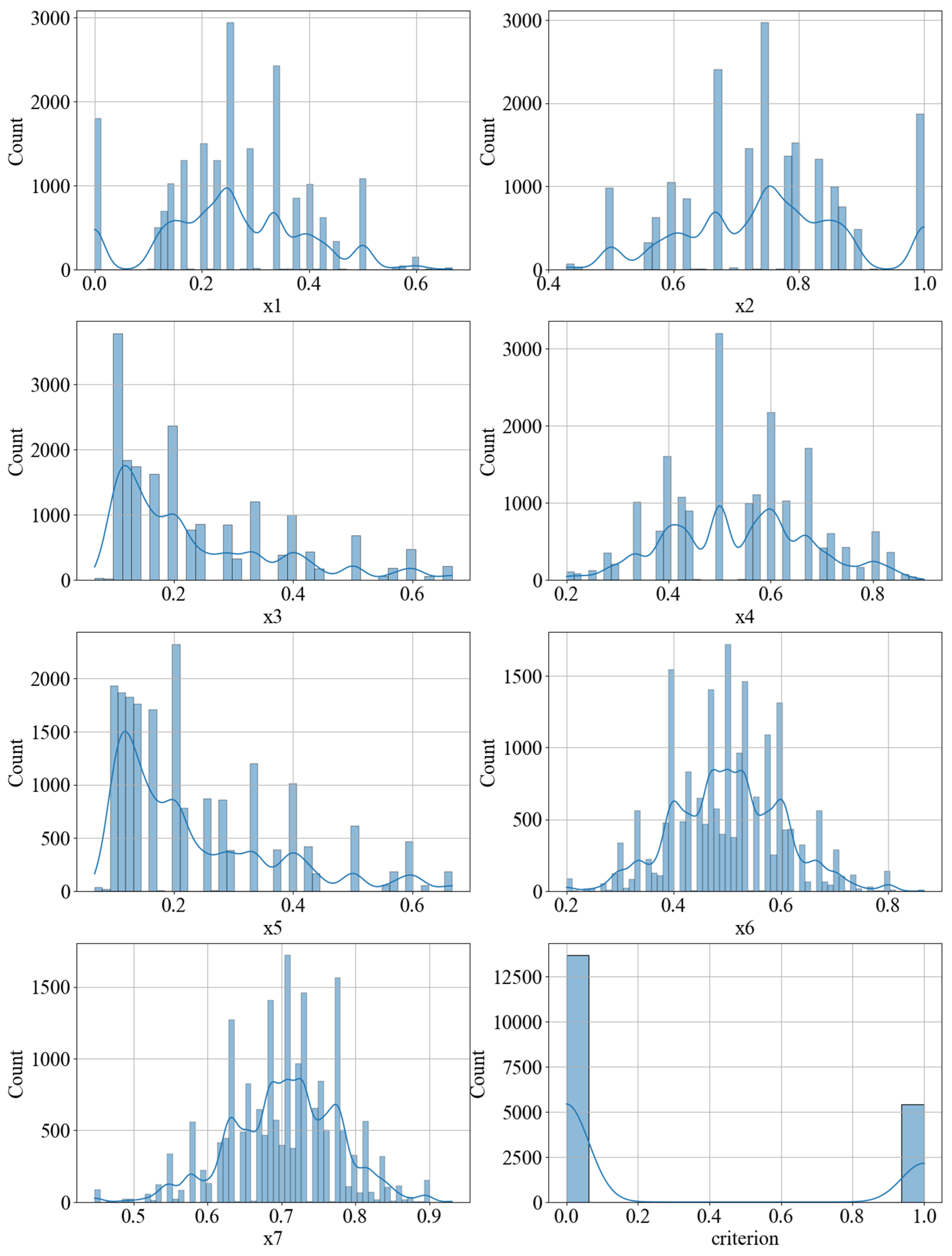
3.2. Analysis of Training Dataset

To train a machine learning model that identifies the fulfillment of Condition (1) based on the parameters in (2), a total of 20,200 randomly generated graphs were used, modeling the structure of the information system. The mentioned parameters were calculated, and the fulfillment of Condition (1) was checked. It is clear that before training any machine learning model on a given dataset, it is necessary to thoroughly explore the dataset. First, potential anomalies need to be identified. For this purpose, we will construct the corresponding frequency histograms (Figure 1).

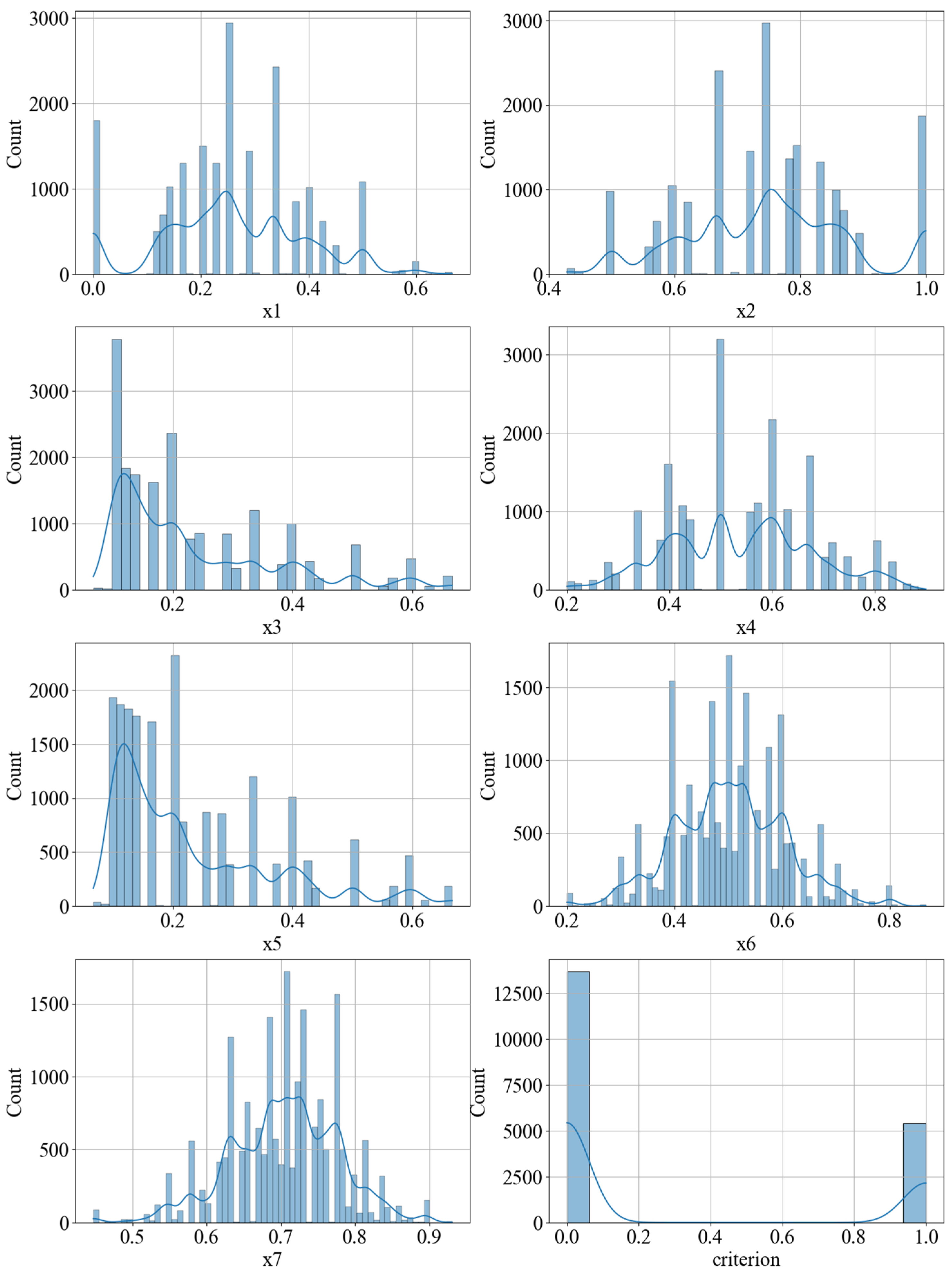
In Figure 1, it is clearly visible that the dataset contains anomalies. Accordingly, it is desirable to remove them, as they could negatively impact the accuracy of predicting the fulfillment of Condition (1) and the subsequent computation of necessary parameters. After removing these anomalies from the dataset, the histograms presented in Figure 1 will appear as shown in Figure 2.

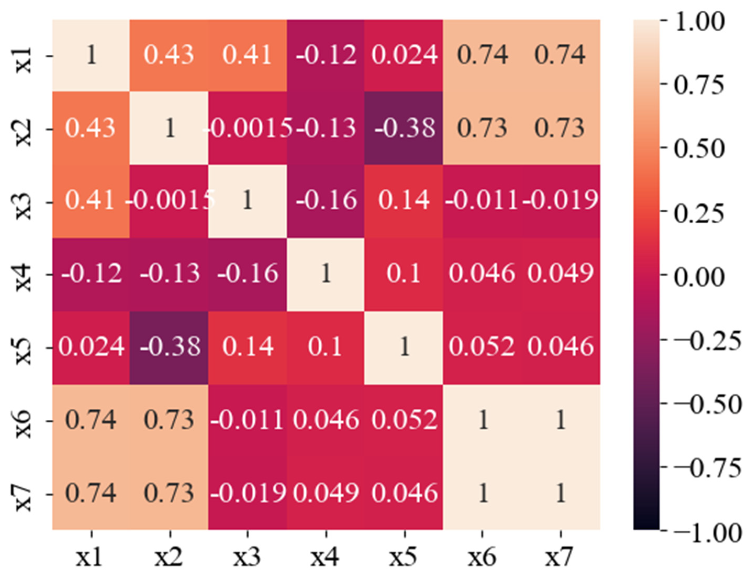
Based on Figure 2, there are no anomalies in the dataset anymore. Thus, it is now possible to investigate the internal relationships between the selected parameters for prediction. To begin with, let us construct a correlation matrix for these parameters and visualize it (Figure 3).

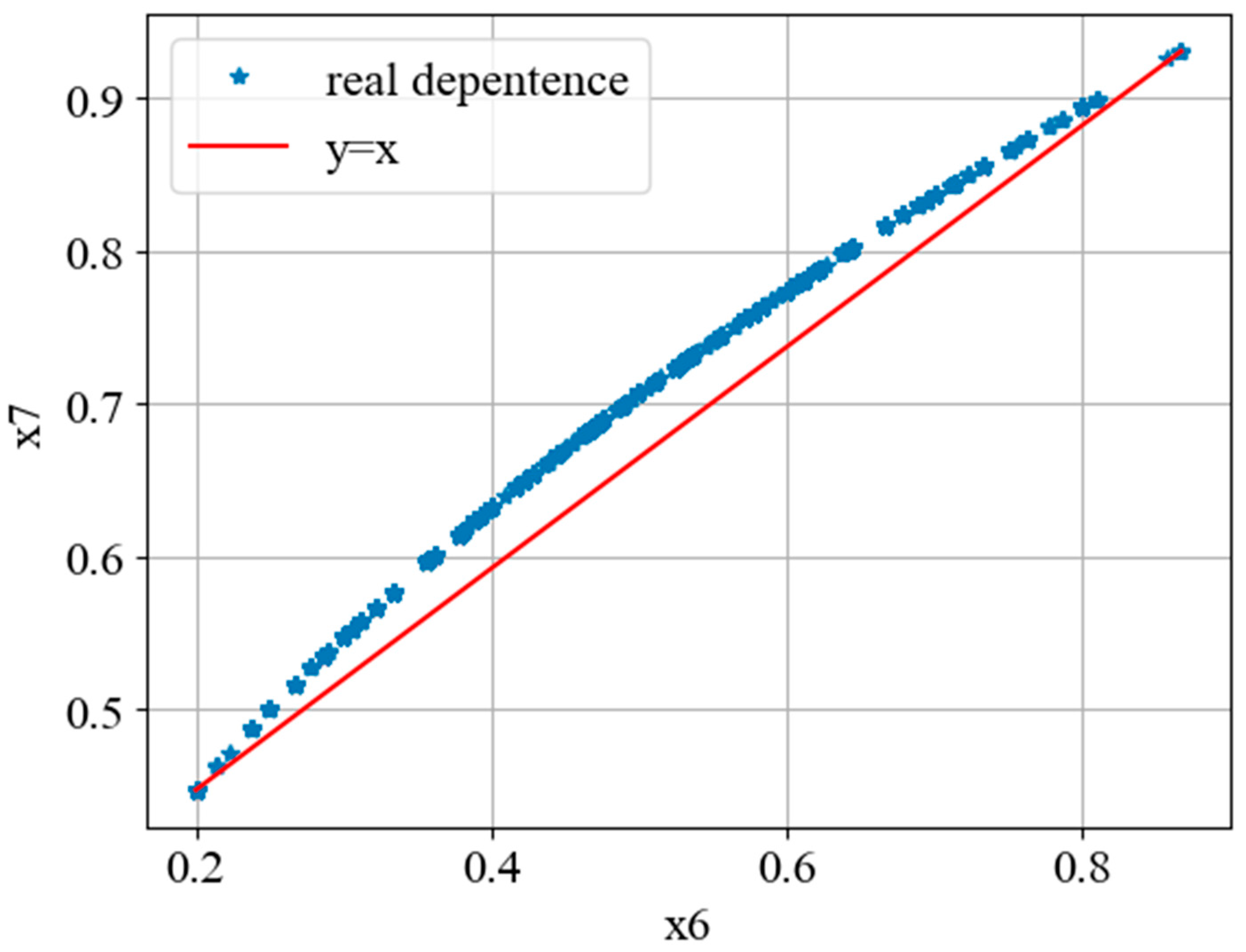
As can be seen in Figure 3, the parameters $x_6$$x_7$ are highly correlated. It is well known that when the correlation coefficient is very close to 1, this indicates a linear relationship between these parameters. To verify that there is indeed a linear dependency between parameters $x_6$$x_7$, we will additionally plot a graph with parameter $x_6$ on the x-axis and parameter $x_7$ on the y-axis (Figure 4).

In Figure 4, it is clearly visible that there is indeed a strong relationship between parameters $x_6$ and $x_7$ and it is nonlinear. If we analyze this more deeply, we may see that the following statement holds:

$$x_7=\sqrt{x_6}.$$

Despite this, it is safe to remove parameter $x_7$ from the dataset. As a result, we now have the following six parameters:

$$x_1={\displaystyle \frac{d_{\min }}{n-1}},x_2={\displaystyle \frac{d_{\max }}{n-1}},x_3={\displaystyle \frac{n_{d=\min }}{n}},x_4={\displaystyle \frac{n_{d\ge mean}}{n}},x_5={\displaystyle \frac{n_{d=\max }}{n}},x_6={\displaystyle \frac{2l}{n\left(n-1\right)}}.$$

(3)

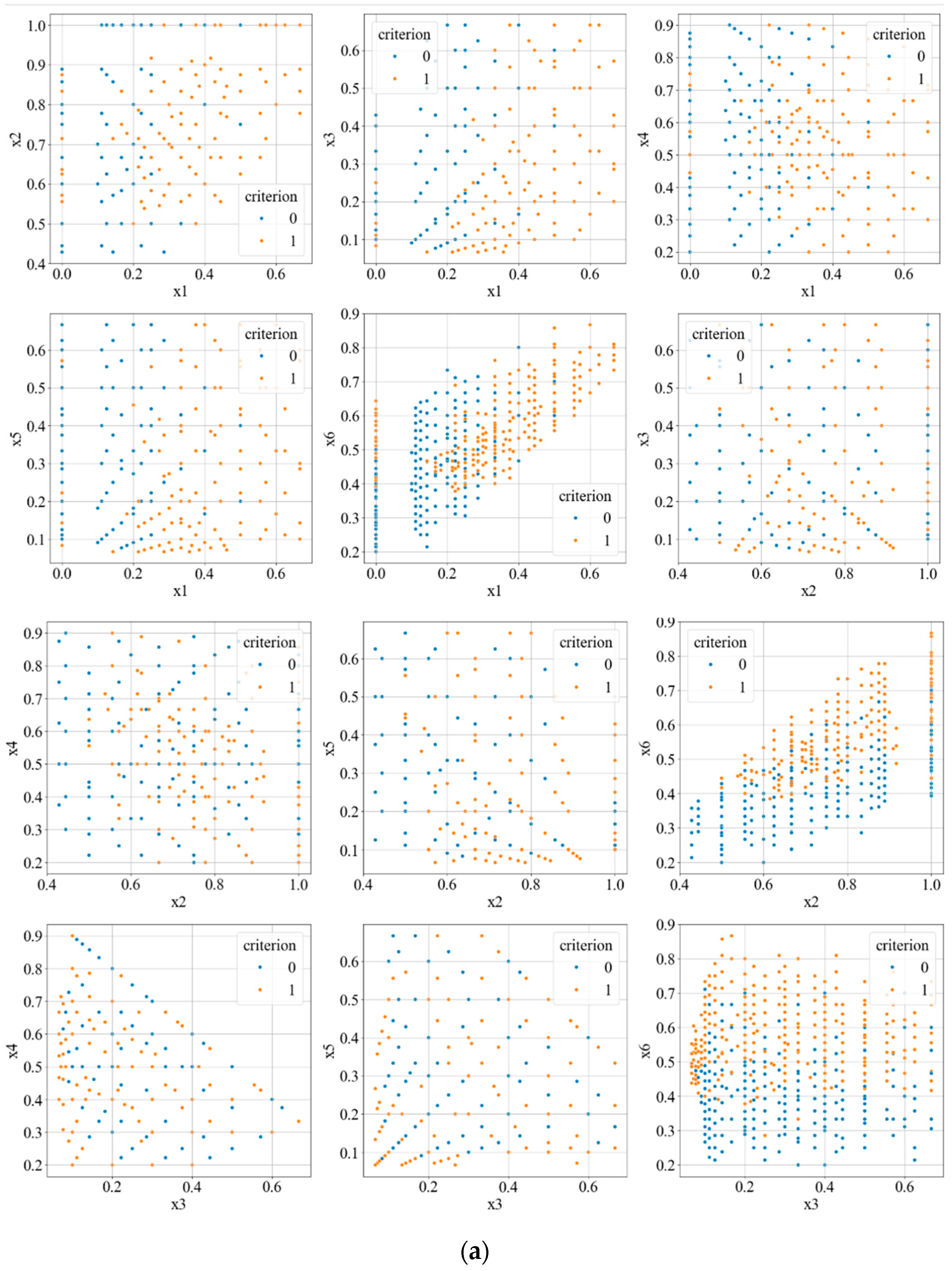
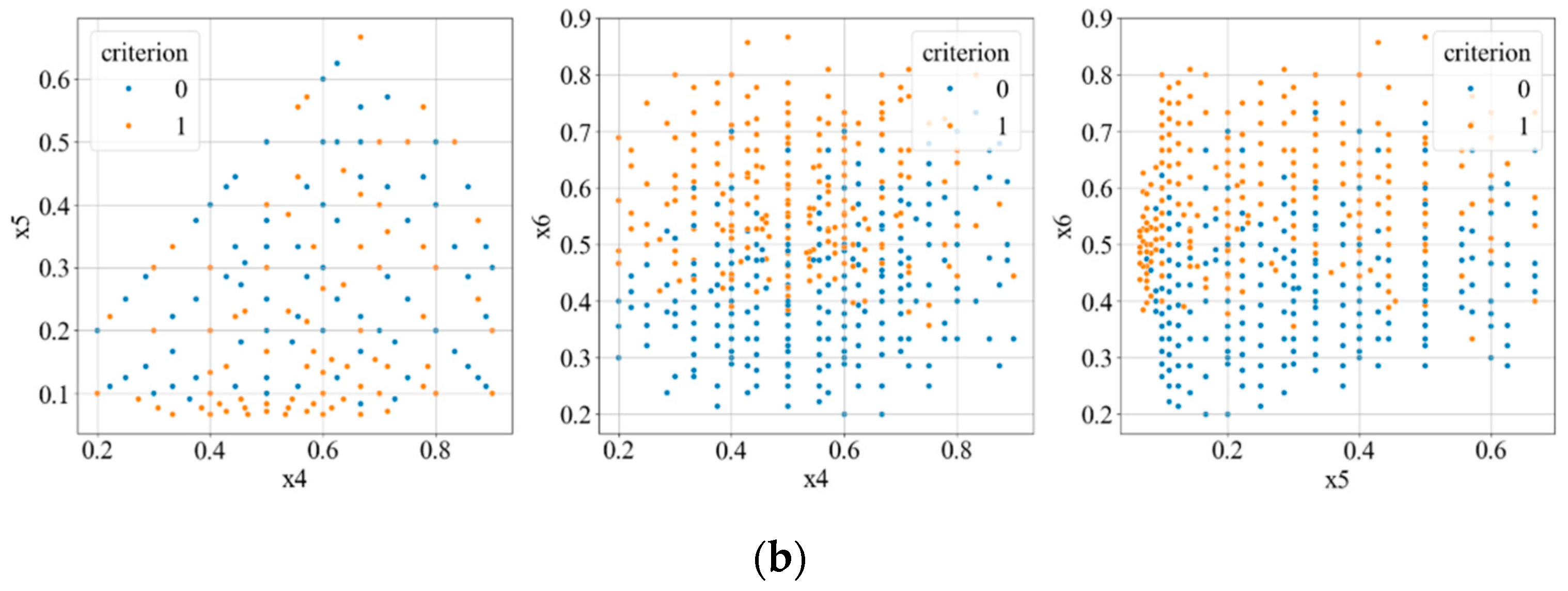
Now, let us investigate how the values of the parameters in the dataset are distributed when Condition (1) is satisfied and when it is not. To do this, we will create scatterplot slices, selecting all pairs of parameters from set (3). The first parameter in each pair will be plotted along the x-axis, and the second along the y-axis (see Figure 5). We will use blue to denote where Condition (1) is met, and red for where it is not met.

In Figure 5a,b, it is clearly visible that by dividing the entire dataset with a certain nonlinear hypersurface, a sufficiently high accuracy in identifying the satisfaction of Condition (1) based on the parameters in (3) can be achieved. In this case, it seems evident that the support vector machine (SVM) method should be used. However, considering the nature of the scatterplots (Figure 5a,b), a significant interest arises in determining how accurately a multilayer perceptron could identify the satisfaction of Condition (1).

3.3. Research on the Applicability of the Support Vector Machine Method for Classifying the Fulfillment of Requirement (1) Based on the Parameters in (3)

When studying the use of the support vector machine with a polynomial kernel, it was decided to explore some cases where the degree of this kernel is higher than one. To study it, let us use three classical metrics of accuracy of classifiers. The first metric is general accuracy (or simply, accuracy), which is usually calculated by the formula

$$accuracy={\displaystyle \frac{TP+TN}{TP+FP+TN+FN}},$$

where $TP$ is the number of correct positive answers, $FP$ is the number of incorrect positive answers, $TN$ is the number of correct negative answers, and $FN$ is the number of incorrect negative answers. The second metric is the true positive rate (in the case of this study, it is the accuracy of identifying the fulfillment of Condition (1)), which is calculated by the formula

$$true\_positive\_rate={\displaystyle \frac{TP}{TP+FP}}.$$

The third metric of marking of classifiers is the true negative rate (in the case of this study it is the accuracy of identifying the non-fulfillment of Condition (1)), which is calculated by the formula

$$true\_negative\_rate={\displaystyle \frac{TN}{TN+FN}}.$$

Using these metrics for studying of the accuracy given by different degrees of the polynomial kernel of the SVM, we obtain the results, which are presented in

Table 1. Accuracy of trained machine learning models based on support vector method with polynomial kernel.

Kernel Power	Accuracy, %	Accuracy of Identifying Fulfillment of Condition (1), %	Accuracy of Identifying Non-Fulfillment of Condition (1), %
2	86.2	84.9	86.5
3	88.3	90.2	87.9
4	89.3	90.7	88.96
5	90.2	96.1	88.7
6	90.7	96.1	89.2

.

As can be seen from Table 1, as the degree of the model kernel increases, the accuracy of correctly identifying the fulfillment of requirement (1) increases. However, such a situation is observed only until the degree of the core is not higher than six. In other words, we may build some surface, described by some function,

$$f\left(x_1,x_2,x_3,x_4,x_5,x_6\right)={\displaystyle \sum _{i_1+i_2+i_3+i_4+i_5+i_6\le 6}{c}_{i_1,i_2,i_3,i_4,i_5,i_6}{x}_1^{i_1}{x}_2^{i_2}{x}_3^{i_3}{x}_4^{i_4}{x}_5^{i_5}{x}_6^{i_6}},$$

on every side, for which the objects will mainly be of one type (points $\left(x_1,x_2,x_3,x_4,x_5,x_6\right)$), which describe the topology of studied information system.

With further increases, the training time grows faster, but the accuracy begins to fall simultaneously. Accordingly, the most optimal option in the case of using the method of support vectors is the use of a polynomial kernel of a degree of 6.

3.4. Research on the Applicability of the Multilayer Perceptron for Classifying the Fulfillment Satisfaction of Requirement (1) Based on the Parameters of (3)

Perceptrons with one to four layers, each with 10 to 100 neurons, were considered within the scope of this study. The activation function in this study was chosen by the authors as ReLU, which is described by the formula

$$\mathrm{Re}LU=\mathrm{Re}LU\left(x\right)=\max \left(0,x\right).$$

It may be augmented by quicker calculations and model training.

As a result, it was found that under the conditions indicated above, it is enough to take a four-layer perceptron, as each layer has 75 neurons. During its testing, the results presented in

Table 2. The accuracy of the described multilayer perceptron.

Accuracy, %	Accuracy of Identifying Fulfillment of Condition (1), %	Accuracy of Identifying Non-Fulfillment of Condition (1), %
91.4	97.7	87.9

were obtained.

During further research, it was found that changing either the number of layers or the number of neurons per layer within the specified range leads to one of two scenarios:

• A decrease in at least one of the metrics listed in Table 2;
• All three metrics listed in Table 2 will increase, but this growth will remain within 0.5%.

On the other hand, comparing the results presented in Table 1 and Table 2, it is easy to see that the use of multilayer perceptrons can provide the same accuracy in identifying the fulfillment of Condition (1) based on the parameters of (3). This raises a logical question: is it possible to improve the accuracy of identification by using support vector machines and multilayer perceptrons together?

If the prediction of the fulfillment of Condition (1) is made by simultaneously using both machine learning models described above, and assuming that Condition (1) is met if either model indicates so, the resulting prediction can indeed be slightly improved (see

Table 3. The accuracy of identifying the fulfillment of Condition (1) with the parallel use of both aforementioned models.

Accuracy, %	Accuracy of Identifying Fulfillment of Condition (1), %	Accuracy of Identifying Non-Fulfillment of Condition (1), %
91.8	97.4	90.3

).

As shown in Table 3, the accuracy of correctly identifying the fulfillment of Condition (1) when using the multilayer perceptron and support vector method in parallel is slightly lower (though this decrease is insignificant) than when using only the multilayer perceptron. However, in this case, the non-fulfillment of Condition (1) is detected with the highest accuracy. This indicates that the combined use of the two machine learning models described above helps to better identify the fulfillment of Condition (1) compared to using each of these models individually.

3.5. Building of Ensembles of Machine Learning Models for Classification of Condition (1) Fulfillment Based on Parameters in (3)

As shown above, using an ensemble of machine learning models can provide better accuracy in identifying the fulfillment of condition (1). Based on this, a logical question arises: can the accuracy of the ensemble comprising the two models described above be improved by adding a third classifier?

To explore this, a classifier based on the k-nearest neighbors (KNN or k-NN) method was selected. In the case of this study, it was ensured that this classifier uses $m$-dimentional Euclidean distance between points $x^1$ and $x^2$, which can be described by the formula

$$\rho \left(x^1,x^2\right)=\sqrt{{\displaystyle \sum _{k=1}^m{\left(x_k^1-x_k^2\right)}^2}}.$$

The tests show that we may use a $k$ parameter equal to 2. In this case, the accuracy of the models was assessed, and the results are presented in

Table 4. The accuracy of identifying the fulfillment of Condition (1) using the k-nearest neighbors method.

Accuracy, %	Accuracy of Identifying Fulfillment of Condition (1), %	Accuracy of Identifying Non-Fulfillment of Condition (1), %
91.2	94.7	90.3

.

Comparing the data presented in Table 3 and Table 4, it becomes evident that the k-nearest neighbors classifier has a slightly lower accuracy than the ensemble of the multilayer perceptron and the support vector classifier with a polynomial kernel. Let us assume that we predict the fulfillment of Condition (1) separately using each of the three described machine learning models. We will consider Condition (1) as fulfilled if at least two of the three models agree on this. The accuracy of such a prediction, obtained through the aforementioned calculations, is presented in

Table 5. The accuracy of identifying the fulfillment of Condition (1) using an ensemble of the support vector method, the k-nearest neighbors method, and the multilayer perceptron in one ensemble.

Accuracy, %	Accuracy of Identifying Fulfillment of Condition (1), %	Accuracy of Identifying Non-Fulfillment of Condition (1), %
91	96.4	89.6

.

Comparing the results presented in Table 3, Table 4 and Table 5, one can conclude that the combined use of all three described models may be impractical. To ensure maximum accuracy, it is more advisable to use either an ensemble of the multilayer perceptron and the classifier based on the support vector method or the classifier based on the k-nearest neighbors method. The first option guarantees higher accuracy, but the second will compute significantly faster. Therefore, the choice between them should depend on what is more critical in a specific situation: speed or accuracy. However, using an ensemble of the three described models will result in the highest calculation time and will not guarantee the highest accuracy.

Comparing the described results, it is logical to ask the following question: if the classifier based on $k$-nearest neighbors gives the best accuracy, what happens if we try to build an ensemble only with these classifiers by analogy with decision trees and random forests? Will we improve the accuracy, as described in Table 4, or not?

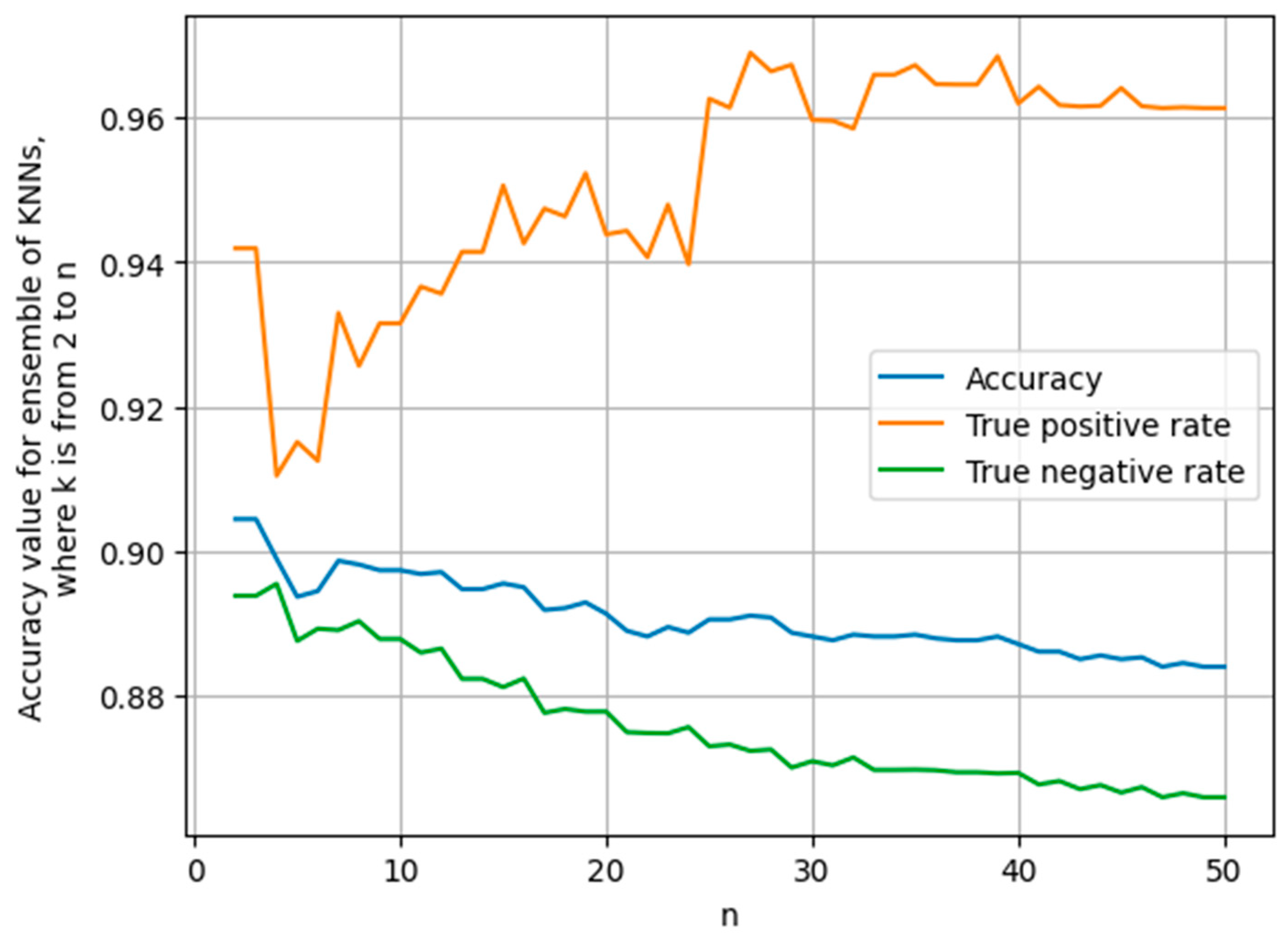
To answer these questions, let us assume that we have an ensemble, which includes all classifiers, based on $k$-nearest neighbors, where $k$ is from 2 to $n$. Now, we must understand how they will depend on the accuracy of the parameter $n$. To achieve this, let us build a schedule (see Figure 6).

In Figure 6, we see two opposite tendencies. The first tendency is an increase in the accuracy of the described ensemble with an increase in parameter $n$: when we increase this parameter, we may have higher accuracy. On the other hand, we see that an increase in parameter $n$ on average results in less accuracy in the identification of the fulfillment of Condition (1) (true positive rate) and less accuracy in the identification of the non-fulfillment of Condition (1) (true negative rate), but this decrease will be little with little deviation in $n$. This may be explained by unbalanced data. This means that this tendency may potentially be corrected. In other words, the previously described ensemble will give higher accuracy than the models described earlier.

If we analogically build an ensemble of machine models which is based on the support vector machine method with the polynomial kernel and build an analogical picture (see Figure 7), we will see that this ensemble does not have the second tendency of the ensemble described previously. This may mean that the ensemble based only on SVMs with different polynomial degrees may better identify Condition (1) using the parameters in (3).

We see that the accuracy (including true positive rate and true negative rate) will increase when the parameter $n$ increases. This means that to guarantee good accuracy in identifying the fulfillment of Condition (1), we may use this ensemble, but not the previously described machine learning models.

4. Discussion

As the experiments show, the usage of classical classifiers and their ensembles with the use of the parameters in (3) as input may give good accuracy in identifying the functional reliability of condition (1). However, the potential accuracy, presented in Table 1, Table 2, Table 3 and Table 4, may be not enough. It would be interesting to try to experiment with other parameters as input (For example, what if we try to add to the parameters in (3) to some other numerical parameters of the topology of the information system?). On the other hand, there is a probability that we may use other ways to solve required tasks [17,18,19,20,21,22,23,24], for example, using ensembles, described above in Figure 6 or Figure 7. But these ensembles have specifics like high training requirements and a high calculation time. As a result, may we solve these problems?

5. Conclusions

This study explored the applicability of the support vector method and multilayer perceptrons for identifying the fulfillment of a functional stability requirement based on Condition (1). Preliminary calibration of each machine learning model was performed, and the accuracy of each model individually and in combination was analyzed. As shown by the presented results, the combined use of multilayer perceptrons and the support vector method provides the best outcomes: only by simultaneously employing these models can the probabilities of both type I and type II errors be kept below 10%. Further investigation revealed that the k-nearest neighbors method with k = 2 can achieve approximately the same level of accuracy. However, any attempt to form an ensemble of all three described machine learning models leads to a decrease in the resulting accuracy of predicting the fulfillment of Condition (1). On the other hand, we may potentially increase the accuracy by using ensembles with classifiers based only on models that use the k-nearest neighbors method. This implies that the combined use of an ensemble with all three models may be impractical. Therefore, it is advisable to use either an ensemble of the multilayer perceptron and the support vector-based classifier (if accuracy is the priority) or the k-nearest neighbors-based classifier (if speed is the priority).

As the experiments show, we may solve the task in another way: for identification of the fulfillment of Condition (1) by using the parameters in (3), we may try to study only ensembles of machine learning models based on the same principles but with different “parameters”. This work studied ensembles of models based on the k-NN method and SVMs with a polynomial kernel with a degree equal to $k$, where $k$ is from 1 (or 2) to $n$. As the tests show, the first variant needs less time for calculations, but the trend of increase in accuracy in the case of an increase in $n$ is unstable. In the case of using SVMs in this context, we may see the opposite situation: an increase in the parameter $n$ guarantees an increase in the accuracy of the ensemble, but such study is very hard to conduct due to computational difficulties.

Initially, the parameters in (2) were chosen as input features. However, analysis of the training dataset showed that the last parameter could be excluded, leaving the parameters in (3) as input features. Preliminary evaluations demonstrated that the parameters in (3) are pairwise uncorrelated and statistically significant at a confidence level of 0.0001. This indicates that they indeed influence the fulfillment of Condition (1). Generally, additional research on other methods of identifying the fulfillment of (1) may potentially continue.

These results may be explained by the following. As we may see in Figure 5a,b, to identify the fulfillment of Condition (1), we may break the hyperspace of points with coordinates $\left(x_1,x_2,x_3,x_4,x_5,x_6\right)$ on parts where there are points, which represent topologies of information systems with a mainly fulfilled or non-fulfilled Condition (1). Because geometrically this break may be realized by SVMs with a polynomial kernel and decision trees, we may use SVMs as classifiers due to their good accuracy (see Table 1) or they may improve ensembles of other classifiers (see Table 2). In a similar geometric sense, one could use the k-NN method. This is why we may use it for identifying the fulfillment of (1) too with better accuracy (see Table 4) than that of the classifier based on multilayer perceptrons (see Table 2). Small differences between the geometric implementation of SVMs and k-NN and their ensembles result in different accuracies in identifying the fulfillment of (1), which is the main reason for the different behavior demonstrated in Figure 6 and Figure 7.

References

- Albini, L.C.; Duarte, E.P.; Ziwich, R.P. A generalized model for distributed comparison-based system-level diagnosis. J. Braz. Comput. 2005, 10, 44–56. [Google Scholar] [CrossRef]
- Barabash, O.V. Construction of Functionally Stable Distributed Information Systems (Ukraine); NAOU: Kyiv, Ukraine, 2004; 226p. [Google Scholar]
- Krishnamachari, B.; Iyengar, S. Distributed Bayesian algorithms for fault-tolerant event region detection in wireless sensor networks. IEEE Trans. Comput. 2004, 53, 241–250. [Google Scholar] [CrossRef]
- Mashkov, V.; Bicanek, J.; Bardachov, Y.; Voronenko, M. Unconventional Approach to Unit Self-diagnosis. Adv. Intell. Syst. Comput. 2020, 1020, 81–96. [Google Scholar] [CrossRef]
- Kalashnyk, G.A.; Kalashnyk-Rybalko, M.A. Signs and criteria of functional stability of the integrated complex of on-board equipment of a modern aircraft and prospective directions of its development. Kharkiv Natl. Univ. Air Force 2021, 68, 7–15. [Google Scholar] [CrossRef]
- Mashkov, V.; Nevliudov, I.; Romashov, Y. Computing the Risk of Failures for High-Temperature Pressurized Pipelines. CEUR Workshop Proc. 2021, 3101, 146–157. [Google Scholar]
- Kravchenko, Y.V.; Nikiforov, S.V. Definition of the problems of the theory of functional stability in relation to application in computer systems. Telecommun. Inf. Technol. 2014, 1, 12–18. [Google Scholar]
- Kravchenko, Y.; Vialkova, V. The problem of providing functional stability properties of information security systems. In Proceedings of the 13th International Conference on Modern Problems of Radio Engineering, Telecommunications and Computer Science (TCSET), Lviv, Ukraine, 23–26 February 2016; pp. 526–530. [Google Scholar] [CrossRef]
- Bellini, E.; Coconea, L.; Nesi, P. A Functional Resonance Analysis Method Driven Resilience Quantification for Socio-Technical Systems. IEEE Syst. J. 2020, 14, 1234–1244. [Google Scholar] [CrossRef]
- Zamrii, I.; Vyshnivskyi, V.; Sobchuk, V. Method of Ensuring the Functional Stability of the Information System Based on Detection of Intrusions and Reconfiguration of Virtual Networks. CEUR Workshop Proc. 2024, 3654, 252–264. [Google Scholar]
- Barabash, O.V.; Musienko, A.P.; Makarchuk, A.V. Comparative analysis of methods for determining the functional stability of information systems using the example of a complete search and the Litvak-Ushakov method. Meas. Comput. Equip. Technol. Syst. 2023, 4, 57–63. [Google Scholar] [CrossRef]
- Cen, J.; Chen, X.; Xu, M.; Zou, Q. Deep finite volume method for high-dimensional partial differential equations. arXiv 2023, preprint. [Google Scholar]
- Zhang, X.; Helwig, J.; Lin, Y.; Xie, Y.; Fu, C.; Wojtowytsch, S.; Ji, S. SineNet: Learning temporal dynamics in time-dependent partial differential equations. arXiv 2025, arXiv:2403.19507v1. [Google Scholar]
- Dulny, A.; Heinisch, P.; Hotho, A.; Krause, A. GrINd: Grid Interpolation Network for Scattered Observations. arXiv 2024, arXiv:2403.19570v1. [Google Scholar]
- Olszewski, S.; Tanasiichuk, Y.; Mashkov, V.; Lytvynenko, V.; Lurie, I. Digital Method of Automated Non-destructive Diagnostics for High-power Magnetron Resonator Blocks. Int. J. Image Graph. Signal Process. 2022, 14, 40–49. [Google Scholar] [CrossRef]
- Mukhin, V.; Komaga, Y.; Zavgorodnii, V.; Zavgorodnya, A.; Herasymenko, O.; Mukhin, O. Social Risk Assessment Mechanism Based on the Neural Networks. In Proceedings of the 2019 IEEE International Conference on Advanced Trends in Information Theory (ATIT), Kyiv, Ukraine, 18–20 December 2019; pp. 179–182. [Google Scholar] [CrossRef]
- Pichkur, V.; Sobchuk, V.; Cherniy, D. Mathematical Models and Control of Functionally Stable Technological Process. In Computational Methods and Mathematical Modeling in Cyberphysics and Engineering Applications; Wiley: Hoboken, NJ, USA, 2024; Volume 1, pp. 101–119. [Google Scholar] [CrossRef]
- Chihara, N.; Takata, T.; Fujiwara, Y.; Noda, K.; Toyoda, K.; Higuchi, K.; Onizuka, M. Effective detection of variable celestial objects using machine learning-based periodic analysis. Astron. Comput. 2023, 45, 100765. [Google Scholar] [CrossRef]
- Hori, K.; Sasaki, Y.; Amagata, D.; Murosaki, Y.; Onizuka, M. Learned Spatial Data Partitioning. In Proceedings of the 6th International Workshop on Exploiting Artificial Intelligence Techniques for Data Management, Seattle, WA, USA, 18 June 2023; p. 3. [Google Scholar] [CrossRef]
- Koval, O.; Barabash, O.; Makarchuk, A.; Havrylko, Y.; Musienko, A.; Salanda, I. Comparison of Two Methods of Signal Smoothing in the Development of Navigation Systems. In Proceedings of the 2023 IEEE 7th International Conference on Methods and Systems of Navigation and Motion Control (MSNMC), Kyiv, Ukraine, 24–27 October 2023; pp. 42–46. [Google Scholar] [CrossRef]
- Makarchuk, A.; Kal’chuk, I.; Kharkevych, Y.; Kharkevych, Y.; Kharkevych, G. Application of Trigonometric Interpolation Polynomials to Signal Processing. In Proceedings of the 2022 IEEE 4th International Conference on Advanced Trends in Information Theory (ATIT), Lviv, Ukraine, 15–17 December 2022; pp. 156–159. [Google Scholar] [CrossRef]
- Mashkov, V.; Fiser, J.; Lytvynenko, V.; Voronenko, M. Diagnosis of intermittently faulty units at system level. Data 2019, 4, 44. [Google Scholar] [CrossRef]
- Pichkur, V.; Sobchuk, V.; Cherniy, D.; Ryzhov, A. Functional Stability of Production Processes as Control Problem of Discrete Systems with Change of State Vector Dimension. Bull. Taras Shevchenko Natl. Univ. Kyiv. Phys. Math. 2024, 1, 105–110. [Google Scholar] [CrossRef]
- Petrivskyi, V.; Shevchenko, V.; Yevseiev, S.; Milov, O.; Laptiev, O.; Bychkov, O.; Fedoriienko, V.; Tkachenko, M.; Kurchenko, O.; Opirskyy, I. Development of a Modification of the Method for Constructing Energy-Efficient Sensor Networks Using Static and Dynamic Sensors. East. Eur. J. Enterp. Technol. 2022, 1, 15–23. [Google Scholar] [CrossRef]