Newly Improved Two-Parameter Ridge Estimators: A Better Approach for Mitigating Multicollinearity in Regression Analysis

Abstract

This study tackles the common issues of multicollinearity arising in regression models due to high correlations among predictor variables, leading to unreliable coefficient estimates and inflated variances, ultimately affecting the model’s accuracy. To address this issue, we introduce four improved two-parameter ridge estimators, named as MIRE1, MIRE2, MIRE3, and MIRE4, which incorporate innovative adjustments such as logarithmic transformations and customized penalization strategies to enhance estimation efficiency. These biased estimators are evaluated through a comprehensive Monte Carlo simulation using the minimum estimated mean square error (MSE) criterion. Although no single ridge estimator performs optimally under all conditions, our proposed estimators consistently outperform existing estimators in most scenarios. Notably, MIRE2 and MIRE3 emerge as the best-performing estimators across a variety of conditions. Their practical utility is further demonstrated through applications to two real-world datasets. The results of the analysis confirm that the proposed ridge estimators offer a reliable and effective approach for improving estimation precision in regression models, as they consistently yield the lowest MSE compared to other estimators.

1. Introduction

Linear regression is a widely used statistical technique for modeling the relationship between a dependent variable and one or more independent variables. The standard linear regression model is expressed as:

$$y=X\varnothing +ϵ,$$

(1)

where $y=\left[\begin{array}{c}{y}_1\\ y_2\\ ⋮\\ y_n\end{array}\right]$ represents an $n\times 1$ vector of response observations, $\mathrm{\varnothing }=\left[\begin{array}{c}{\mathrm{\varnothing }}_1\\ {\mathrm{\varnothing }}_2\\ ⋮\\ {\mathrm{\varnothing }}_p\end{array}\right]$ is a $p\times 1$ vector of unknown regression coefficients, $X=\left[\begin{array}{cccc}{x}_{11}& x_{12}& \dots & x_{1p}\\ x_{21}& x_{22}& \dots & x_{2p}\\ ⋮& ⋮& \ddots & ⋮\\ x_{n1}& x_{n2}& \dots & x_{np}\end{array}\right]$ is an $n\times p$ matrix of predictor observations, and $\mathsf{ϵ}=\left[\begin{array}{c}{ϵ}_1\\ {ϵ}_2\\ ⋮\\ {ϵ}_n\end{array}\right]$ is an $n\times 1$ vector of error terms.

The ordinary least squares (OLS) solution for estimating the regression coefficients is given in Equation (2):

$${\widehat{\varnothing }}_{ols}=\left[\begin{array}{c}{\widehat{\varnothing }}_1\\ {\widehat{\varnothing }}_2\\ ⋮\\ {\widehat{\varnothing }}_p\end{array}\right]={\left(X^{\prime }X\right)}^{-1}{X}^{\prime }y.$$

(2)

However, OLS estimates can become unstable in the presence of multicollinearity among predictor variables, leading to inflated variances of regression coefficients [1]. Ridge regression is a robust alternative to address this problem by introducing a penalty term to the OLS method. The ridge regression estimator is defined in Equation (3) as:

$${\widehat{\varnothing }}_{Rd}={\left(X^{\prime }X+kI\right)}^{-1}{X}^{\prime }y.$$

(3)

In this equation, $I$ is the identity of the order p × p and $k$is a positive scalar usually called a ridge parameter. The ridge parameter is the level of shrinkage used on the coefficient estimates and the choice of $k$ is very integral in the determination of the tradeoff between bias and variance.

To enhance ridge regression’s flexibility, a two-parameter ridge estimator has been proposed [2]. This generalized form introduces a scaling factor $q$ and is expressed in Equation (4) as:

$${\widehat{\varnothing }}_{\left(q,k\right)}={q\left(X^{\prime }X+kI\right)}^{-1}{X}^{\prime }y.$$

(4)

Here, $q$ is a scaling factor, and the presence of both $q$ and $k$ gives a more flexible class of solutions to the ridge regression problem. The scaling factor $q$ can be computed as:

$$\widehat{q}={\displaystyle \frac{{\left(X^{\prime }y\right)}^{\prime }{\left(X^{\prime }X+kI\right)}^{-1}{X}^{\prime }y}{{\left(X^{\prime }y\right)}^{\prime }{\left(X^{\prime }X+kI\right)}^{-1}{X}^{\prime }X{\left(X^{\prime }X+kI\right)}^{-1}{X}^{\prime }y}}.$$

(5)

Equation (4) reduces to the conventional OLS and ridge regression estimating equation when $q=1$ and $k=k$ or $k=0$. Therefore, the new idea of the two-parameter ridge estimator is helpful in providing a better solution to the problem of multicollinearity in regression analysis. Ref. [3] provided further information about the cross-sectional analysis of variance and ordinary least square estimator and its development to enhance multicollinearity.

Several studies have explored specific improvements in ridge regression. Ref. [4] conducted a Monte Carlo evaluation of various ridge-type estimators, providing empirical comparisons of their performance. Further, the work of [5] offered refined methods for selecting ridge parameters, essential for optimizing model accuracy. Ref. [6] also evaluated new ridge regression estimators, contributing to the empirical understanding of these methods.

The development of ridge regression has also crossed into specialized fields. For instance, Ref. [7] examined its role in logistic regression, while [8] focused on improved ridge regression estimators for logistic models, offering more robust options in binary classification problems. Ref. [9] reviewed ridge-type estimators, highlighting raise estimators for geometric data perturbation and parameter selection. More recently, Ref. [10] developed new ridge estimators to examine the severe multicollinearity data. The authors of [11] further explored robust ridge estimators, particularly under conditions of multicollinearity and the presence of outliers. These robust methods provide a more reliable estimation framework in real-world datasets.

Modern applications of ridge regression are evident in various fields, including environmental science and econometrics. For example, Ref. [12] developed a carbon price forecasting model based on Lasso regression and optimal integration, blending traditional ridge regression with machine learning techniques for improved forecasting accuracy. Ref. [10] developed two-parameter estimators to address linear regression models with correlated predictors. Additionally, the work of [13] introduced two-parameter ridge estimators, further advancing ridge regression in dealing with correlated predictors.

Although significant progress has been made in the development of ridge estimators, no single ridge estimator has consistently demonstrated optimal performance across varying multicollinearity conditions. Existing estimators often excel in specific scenarios but lack robustness and adaptability when applied to diverse datasets. To fill this gap, this study proposes four novel ridge estimators referred to as MIRE1, MIRE2, MIRE3, and MIRE4. These estimators are rigorously evaluated through comprehensive Monte Carlo simulations and compared to other existing estimators using MSE criterion. The results of the analysis indicate that the proposed estimators offer superior performance, particularly in multicollinear datasets, providing a significant contribution to the ongoing development of robust regression techniques. This work fills a critical gap in the literature by offering a set of estimators that provide more reliable performance across diverse datasets, marking a significant advancement in the development of more flexible and effective regression techniques.

The article is structured as follows. Section 2 discusses ridge regression methodology, introducing the proposed and existing estimators. Section 3 covers the simulation study and results analysis. Section 4 applies the estimators to two real datasets, and Section 5 concludes the study.

2. Statistical Methodology for Ridge Regression

To simplify the model, we can express Equation (1) in its canonical form as:

$$y=Z\phi +ϵ,$$

(6)

where

• $Z=XD$, a transformed design matrix.
• $\phi =D^{\prime }\varnothing$, where $D$ is an orthogonal matrix containing the eigenvectors of $X^{\prime }X$.
• $\varnothing$ is the parameter vector, and ϵ represents the noise.
• $D^{\prime }D=I_p$ ensuring orthogonality, with $I_p$ being the identity matrix.
• The transformation $Z=XD$ aligns $Z$ with the principal components of $X$.

Additionally, we define:

$$\Lambda =D^{\prime }{X}^{\prime }XD.$$

Here, $\Lambda$ is a diagonal matrix of the eigenvalues ${\lambda }_1,{\lambda }_2,\dots ,{\lambda }_p$ arranged in ascending order.

Using the canonical form, ridge regression estimators can be rewritten in terms of the transformed parameters $\phi$ instead of $\varnothing$.

The standard OLS estimator in canonical form becomes:

$$\widehat{\phi }={\Lambda }^{-1}{Z}^{\prime }y.$$

(7)

Here, ${\Lambda }^{-1}$ directly scales the projections $Z^{\prime }y$ by the reciprocal of eigenvalues, leading to instability when ${\lambda }_i$ are small.

The ridge regression estimator in its canonical form is given as:

$${\widehat{\phi }}_k={\left(\Lambda +k{I}_p\right)}^{-1}{Z}^{\prime }y.$$

(8)

This formulation ensures stability by adding $k$ to each eigenvalue, effectively shrinking the coefficients corresponding to small eigenvalues.

The two-parameter ridge regression estimator in canonical form is:

$${\widehat{\phi }}_{q,k}=q{\left(\Lambda +k{I}_p\right)}^{-1}{Z}^{\prime }y.$$

(9)

2.1. Ridge Estimators

In this section, we discuss both existing ridge regression techniques and the newly proposed ridge estimators.

2.1.1. Existing Ridge Estimators

Several ridge estimators were introduced in the literature; here, we will consider some of them that are relevant to our study. In the following, ${\widehat{\sigma }}^2$ represents the estimated error variance of the regression model and ${\lambda }_{max}$ denotes the largest eigenvalue of the covariance matrix $X^{\prime }X.$

The authors of [1] introduced the first ridge estimator, referred to as HK. It is defined as:

$${\widehat{k}}_{HK}={\displaystyle \frac{{\widehat{\sigma }}^2}{{\widehat{\phi }}_{Max}^2}}, \mathrm{where} {\widehat{\phi }}_{Max}=Max({\widehat{\phi }}_1 , {\widehat{\phi }}_2 , \dots , {\widehat{\phi }}_p).$$

(10)

Ref. [14] modified the HK estimator by incorporating the number of predictors and the modified version is referred to as the HKB estimator. Its form is:

$${\widehat{k}}_{HKB}={\displaystyle \frac{p {\widehat{\sigma }}^2}{{\sum }_{i=1}^p{\widehat{\phi }}_i^2}}.$$

(11)

Kibria [6] introduced three ridge estimators based on averaging techniques, referred to as KAM (Arithmetic Mean), KGM (Geometric Mean), and KMed (Median). These estimators are defined as follows:

$$\begin{array}{c}\mathrm{K}\mathrm{A}\mathrm{M}={\widehat{k}}_{AM}={\displaystyle \frac{1}{p}}{\sum }_{i=1}^p{\displaystyle \frac{{\widehat{\sigma }}^2}{{\widehat{\phi }}_i^2}},\\ \mathrm{K}\mathrm{G}\mathrm{M}={\widehat{k}}_{GM}={\displaystyle \frac{{\widehat{\sigma }}^2}{{\left({\prod }_{i=1}^p{\widehat{\phi }}_i^2\right)}^{\frac{1}{p}}}},\\ \mathrm{K}\mathrm{M}\mathrm{e}\mathrm{d}={\widehat{k}}_{Med}=\mathrm{M}\mathrm{e}\mathrm{d}\left({\displaystyle \frac{{\widehat{\sigma }}^2}{{\widehat{\phi }}_i^2}}\right).\end{array}$$

(12)

Researchers in [15] focused on eigenvalue-based adjustments to introduce a new estimator referred to as KMS with the following expression:

$${\widehat{k}}_{KMS}={\displaystyle \frac{{\mathsf{\lambda }}_{\max }{\sum }_{i=1}^p\left|{\widehat{\phi }}_i\right|}{\left\{\frac{{\widehat{\sigma }}^2}{{\widehat{\phi }}_{Max}^2}\right\}}}.$$

(13)

In [16], an enhanced ridge regression method was proposed by introducing a two-parameter ridge estimator, termed LC estimator in this study. The ridge parameter $k$ is determined through Equation (10), while the second parameter $q$ is derived using Equation (5). Similarly, the authors of [3] developed another two-parameter ridge estimator, referred to as TK estimator, with optimal values for $q$ and $k$ calculated using Equation (14).

$$\begin{array}{c}{\widehat{q}}_{opt}={\displaystyle \frac{{\sum }_{i=1}^p{\widehat{\phi }}_i^2\frac{{\mathsf{\lambda }}_i}{{\mathsf{\lambda }}_i+k}}{{\sum }_{i=1}^p\frac{{\widehat{\sigma }}^2{\mathsf{\lambda }}_i+{\widehat{\phi }}_i^2{\mathsf{\lambda }}_i^2}{{\left({\mathsf{\lambda }}_i+k\right)}^2}}} ,\\ {\widehat{k}}_{opt}={\displaystyle \frac{{\widehat{q}}_{opt}{\sum }_{i=1}^p\frac{{\widehat{\sigma }}^2}{{\mathsf{\lambda }}_i}+\left({\widehat{q}}_{opt}-1\right) {\sum }_{i=1}^p{\widehat{\phi }}_i^2{\mathsf{\lambda }}_i^2}{{\sum }_{i=1}^p{\widehat{\phi }}_i^2{\mathsf{\lambda }}_i}} .\end{array}$$

(14)

The authors of [17] proposed three modified versions of the two-parameter ridge estimators, referred to as MTPR1, MTPR2, and MTPR3, which are defined as follows:

$$\begin{array}{c}\mathrm{M}\mathrm{T}\mathrm{P}\mathrm{R}1:{\widehat{k}}_{AM}^{*}={\displaystyle \frac{\sum _{i=1}^p{k}_i^{*}}{p}},\\ \mathrm{M}\mathrm{T}\mathrm{P}\mathrm{R}2:{\widehat{k}}_{GM}^{*}={\left(\prod _{i=1}^p{k}_i^{*}\right)}^{{\displaystyle \frac{1}{p}}},\\ \mathrm{M}\mathrm{T}\mathrm{P}\mathrm{R}3:{\widehat{k}}_{HM}^{*}={\displaystyle \frac{p}{\sum _{i=1}^p\frac{1}{k_i^{*}}}}.\end{array}$$

(15)

In each instance above, the adjusted $k$-value for the $i^{th}$ predictor is computed as:

$$k_i^{*}=w_i{\widehat{k}}_{opt},$$

${\widehat{k}}_{opt}$ is the optimal $k$-value determined through an optimization process in these ridge estimation models. The weighted $w_i$ is defined as:

$$w_i={\displaystyle \frac{{\mathit{\lambda }}_{\mathit{i}}}{\left|{\phi }_i\right|}},$$

where $\left|{\phi }_i\right|$is the absolute regression coefficient, and ${\mathit{\lambda }}_{\mathit{i}}$ is its corresponding eigenvalue of $X^{\prime }X.$

The $k\text{-}$values of the estimators mentioned above are used to determine $q$ from Equation (14).

The above competitive ridge estimators, HK, HKB, KAM, KGM, KMed, KMS, LC, TK, MTPR1, MTPR2, and MTPR3, were assessed and compared with our newly proposed ridge estimators, MIRE1, MIRE2, MIRE3, and MIRE4 using simulations and real-life datasets exhibiting severe multicollinearity.

2.1.2. New Proposed Ridge Estimators

We introduce four modified Lipovetsky–Conklin ridge (MLCR) estimators, which integrate the methodologies of [3,16] to determine the optimal values of $q$ and $k$. Given the maximum eigenvalue ${\mathsf{\lambda }}_{max}$, the $k$-values for our four estimators are outlined as follows:

$$\mathrm{M}\mathrm{I}\mathrm{R}\mathrm{E}1:k_1=\left.\left(log\sqrt{\left(1+{\displaystyle \frac{1}{p}}{\sum }_{i=1}^p\left(({\mathsf{\lambda }}_i\left|{\widehat{\phi }}_i\right|{)}^2\right)\right)}\right.\right)\left({\displaystyle \frac{{\widehat{\sigma }}^2}{{\widehat{\phi }}_{max}^2}}\right),$$

(16)

$${\mathrm{M}\mathrm{I}\mathrm{R}\mathrm{E}2:k}_2={\displaystyle \frac{{\mathsf{\lambda }}_{max}}{\sqrt{{\widehat{\phi }}_i}}} \left({\displaystyle \frac{{\widehat{\sigma }}^2}{{\widehat{\phi }}_{max}^2}}\right),$$

(17)

$${\mathrm{M}\mathrm{I}\mathrm{R}\mathrm{E}3:k}_3={\mathsf{\lambda }}_{max} log(1+\left|{\widehat{\phi }}_i\right|),$$

(18)

$${ \mathrm{M}\mathrm{I}\mathrm{R}\mathrm{E}4:k}_4={\displaystyle \frac{{\mathsf{\lambda }}_{max}}{{\left|{\widehat{\phi }}_i\right|}^2}} \left({\displaystyle \frac{{\widehat{\sigma }}^2}{{\widehat{\phi }}_{max}^2}}\right).$$

(19)

Equation (5) is used for calculating the estimated $q$-value. Based on these calculations, our four novel two-parameter ridge estimators, denoted as MIRE1, MIRE2, MIRE3, and MIRE4, can be obtained.

2.1.3. Performance of Estimators Under Mean Square Error

The performance of the proposed estimators was evaluated using the Mean Squared Error (MSE) criterion. This approach has been widely employed in previous studies, including [13,18] to analyze the effectiveness of various estimators. The MSE is represented by the following expression:

$$MSE\left(\widehat{\phi }\right)=E\left[(\widehat{\phi }-\phi {)}^{\prime }\left(\widehat{\phi }-\phi \right)\right]$$

(20)

$$={\displaystyle \frac{1}{p}}{\sum }_{i=1}^p({\widehat{\phi }}_i-\phi {)}^2$$

(21)

Since theoretical comparisons of ridge estimators based on MSE are complex, the ridge estimators, shown in Equation (10) to Equation (19), were evaluated through Monte Carlo simulations as described in the following section.

3. Monte Carlo Simulations

This section outlines the Monte Carlo simulation process used to assess the performance of the proposed ridge estimators in comparison to OLS and other existing ridge estimators.

3.1. Simulation Study

This study investigates ridge regression performance by generating predictor variables under controlled multicollinearity settings. Predictors $x_{ij}$ were simulated using the following equation, a process adopted by many researchers, including [19,20], to generate predictor variables as shown in Equation (22).

$$x_{ij}=\sqrt{1-{\rho }^2}. z_{ji}+\rho z_{jp}, i=\mathrm{1,2},\dots ,p and j=\mathrm{1,2},\dots ,n ,$$

(22)

where $x_{ij}$ represents the $j^{th}$ observation for the $i^{th}$ predictor, $\rho$ denotes the correlation between predictors, $z_{ji}$ are independent random samples drawn from a standard normal distribution, $p$ is the total number of predictors, and $n$ represents the sample size. To examine a range of multicollinearity conditions, $\rho$ was varied across $0.80, 0.90, 0.95, \mathrm{a}\mathrm{n}\mathrm{d} 0.99$. Sample sizes $(n=20, 50, 100)$ and predictor counts $(p=4, 10)$ were selected to assess model robustness across different dimensionalities.

The response variable $y_j$ is generated using the following model:

$$y_j={\phi }_0+{\phi }_1{x}_{j1}+{\phi }_2{x}_{j2}+\dots +{\phi }_p{x}_{jp}+{\mathsf{ϵ}}_j , j=1,2\dots ,n$$

(23)

where ${\phi }_0$ is the intercept (set to zero), ${\phi }_i$ are the regression coefficients chosen based on optimal conditions, and ${\mathsf{ϵ}}_j$ is an error term drawn from a normal distribution with variance ${\sigma }^2$. Error variance was examined at four levels: ${\sigma }^2=0.4, 1, 5, \mathrm{a}\mathrm{n}\mathrm{d} 10$. The regression coefficients ${\phi }_i$ were calculated by identifying the optimal direction, as outlined in the methodology proposed in [21]. Algorithm 1 was used to execute the estimated MSE of the estimators.

Algorithm 1: MSE Computation.

i. Generate and standardize the matrix of independent variables using Equation (22). ii. Calculate eigenvalues $\left({\lambda }_1,\dots ,{\lambda }_p\right)$ and eigenvectors $\left(e_1,\dots ,e_p\right)$ of $X^{\prime }X$, ensuring $\sum _{i=1}^p{\mathsf{\lambda }}_{\mathrm{i}}$ $=p.$ iii. Determine regression coefficients $\phi$ in canonical form using $\phi$ $={\lambda }_{\mathrm{m}\mathrm{a}\mathrm{x}} P$, where $P=\left[e_1,\dots ,e_p\right]$ and ${\lambda }_{\mathrm{m}\mathrm{a}\mathrm{x}}$corresponds to the largest eigenvalue, and generate random error terms based on distributions $N\left(\mathrm{0,1}\right)$. iv. Compute the dependent variable values using Equation (9). v. Calculate OLS and ridge regression estimates for $\phi$ using appropriate equations. vi. Repeat steps i–v for $N$ = 10,000 Monte Carlo iterations. vii. Calculate the MSE for all estimators using:

$MSE\left(\widehat{\phi }\right)={\displaystyle \frac{1}{N}}\sum _{j=1}^N\left[({\widehat{\phi }}_j-\phi {)}^{\prime }\left({\widehat{\phi }}_j-\phi \right)\right]$.  (24)

A simulation study with $N=\mathrm{10,000}$ runs was performed to evaluate the MSE for varying values of $\rho$, $n$, and $p$ using R programming language. The results are summarized in Table A1, Table A2, Table A3, Table A4, Table A5, Table A6 and Table A7 in Appendix A, where bolded values indicate the lowest MSE for each estimator, highlighting higher accuracy and improved predictive performance. A detailed analysis and discussion of these results are provided in following section.

3.2. Discussion of the Results

The performance of the newly proposed estimators (MIRE1, MIRE2, MIRE3, and MIRE4), OLS, and other existing estimators was tested using the estimated MSE as the evaluation criterion. The study comprehensively considered varying sample sizes $(n=20, 50, 100)$, numbers of predictors $(p=4, 10)$, levels of correlation $\left(\rho \right)$, and error variances $\left({\sigma }^2\right)$. The simulation findings can be highlighted in the following points.

Proposed Estimators (MIRE1, MIRE2, MIRE3, and MIRE4): Across different scenarios of $n, p, \rho , \mathrm{a}\mathrm{n}\mathrm{d} {\sigma }^2$, the proposed estimators consistently achieved lower MSE values compared to most existing estimators. Among the proposed estimators, MIRE3 often outperformed MIRE1 and MIRE2, particularly in scenarios with higher correlations $(\rho \ge 0.95)$ and larger numbers of predictors$\left(p=10\right)$. This suggests that MIRE3 is better suited to handling multicollinearity in these scenarios.

Existing Estimators: OLS and estimator KAM estimator showed higher MSE values in nearly all scenarios, particularly when $\rho$ and $p$ are large. This highlights their sensitivity to multicollinearity. Other existing estimators such as KMed, KMS, and HK tended to perform better than other existing estimators but were generally outperformed by our proposed MIRE estimators. The performance of the estimators LC, TK, MTPR1, MTPR2, and MTPR3 was heavily dependent on the combination of $n, p$, and ${\sigma }^2$. For instance, lc and tk achieved lower mse in smaller error variances (${\sigma }^2=0.40$); however, they fell short in scenarios with high${\sigma }^2$.

Impact of correlation ($\mathsf{\rho }$): As the correlation increased, the challenge of multicollinearity becomes more pronounced. The proposed estimators demonstrated robustness under high correlations $(\mathsf{\rho }=0.95,0.99)$, maintaining lower mse values compared to other estimators. The ols and hk estimators suffered significantly under high $\mathsf{\rho }$, with their mse values increasing dramatically, particularly when $\mathrm{p}=10$.

Impact of Sample Size ($\mathbf{n}$): Larger sample sizes $(\mathrm{n}=50,100)$ generally led to reduced MSE values across all estimators, reflecting the benefits of increased data availability. For small sample sizes $(\mathrm{n}=20)$, our MIRE estimators remained competitive, with MTPR3 emerging as particularly reliable.

The performance gap between the proposed and existing estimators narrowed with increasing $\mathrm{n}$; however, the proposed estimators maintained their advantage, especially in high-dimensional settings $(\mathrm{p}=10)$.

Impact of Predictors ($\mathbf{p}$): Increasing the number of predictors ($\mathrm{f}\mathrm{o}\mathrm{r} \mathrm{e}\mathrm{x}\mathrm{a}\mathrm{m}\mathrm{p}\mathrm{l}\mathrm{e} \mathrm{p}=10)$ exacerbated multicollinearity, leading to a noticeable rise in MSE for existing estimators. The proposed estimators showed their strength in handling high-dimensional data, with MIRE3 consistently delivering the lowest MSE among all methods.

Impact of Error Variance (${\mathit{\sigma }}^2$): A smaller error variance (${\sigma }^2=0.40)$ favored all estimators, resulting in a reduced MSE. As ${\sigma }^2$ increased, the gap between the proposed and existing estimators widened, highlighting the robustness of MIRE1, MIRE2, MIRE3, and MIRE4 under high error variances.

The summary of Table A7 (provided in Appendix A) demonstrates the performance of ridge estimators across varying sample sizes (n), error variances ($\sigma$), and multicollinearity levels $\left(\rho \right)$, showcasing that the proposed estimators (MIRE1, MIRE2, MIRE3, and MIRE4) performed best in 30 out of 32 scenarios. They exceled under severe multicollinearity $(\rho >0.95$) and high noise $({\sigma }^2=5, 10)$. For a small sample $(n=20)$, MTPR1 performed well in five cases under low noise, while MIRE3 and MIRE2 dominated in eight scenarios as noise increases. For larger samples $(n=50, 100)$, MIRE3 and MIRE2 achieved the lowest MSE in $15$ scenarios, with MTPR’s estimators excelling in three low-noise cases. These results underline the adaptability and consistency of the proposed estimators, particularly in challenging multicollinear settings.

4. Real-Life Applications

The first dataset we considered is the Blood Pressure dataset, sourced from Applied Regression Analysis [22], which serves as a benchmark in regression analysis. The second dataset, Acetylene Conversion data, was taken from [23] and foundational research by [24]. We utilized these two real datasets to evaluate the performance of the proposed and existing ridge estimators.

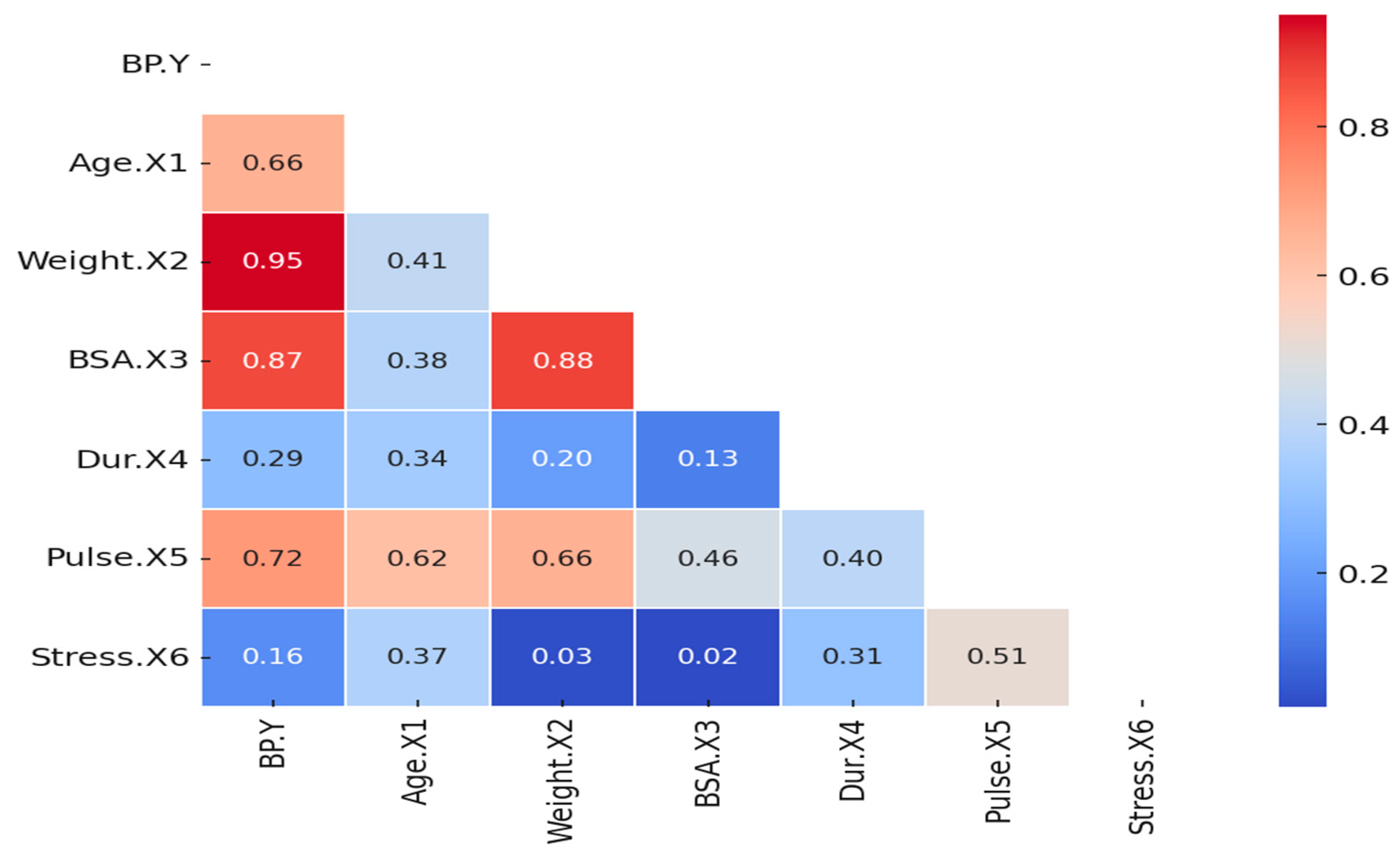
4.1. Blood Pressure Patients Dataset

The Blood Pressure (BP) Patients dataset includes 20 patients and seven variables, with BP as the response variable and six predictors, age ($X_1)$, weight ($X_2)$, BSA ($X_3)$, duration ($X_4)$, pulse ($X_5)$, and stress ($X_6$). We fit a linear regression model using BP as the dependent variable and the six predictors as independent variables. The linear regression model can be expressed as:

$$y={\phi }_0+{\phi }_1{X}_1+{\phi }_2{X}_2+{\phi }_3{X}_3+{\phi }_4{X}_4+{\phi }_5{X}_5+{\phi }_6{X}_6+\mathsf{ϵ},$$

where ${\phi }_0$ is the intercept and ${\phi }_1$, ${\phi }_2$, ${\phi }_3$, ${\phi }_4, {\phi }_5, \mathrm{a}\mathrm{n}\mathrm{d} {\phi }_6$ are the coefficients for each predictor, and ϵ represents the error term.

To check for multicollinearity in the Blood Pressure Patients dataset, we use the Condition Number $\left(CN\right)$, Eigenvalues, Variance Inflation Factors (VIFs), and Heatmap pairs wise correlation display. A $\mathrm{C}\mathrm{N}$ above 30, small eigenvalues, or $\mathrm{V}\mathrm{I}\mathrm{F}$ values exceeding 5 indicate multicollinearity, which can distort regression results. Addressing multicollinearity may require methods such as ridge regression.

The dataset demonstrates severe multicollinearity, evidenced by a high value of $CN$(1746.33) and a smallest eigenvalue of 0.0022, indicating near-linear dependency among predictors. VIF values are also excessively high for key variables such as BP (259.76), age (29.02), and weight (161.35). Furthermore, Figure 1 reveals strong positive correlations between BP and predictors such as weight and BSA, while stress shows weaker correlations with other variables. These findings confirm the significant multicollinearity present, which can lead to unstable and unreliable regression coefficient estimates. To mitigate this issue, the newly proposed and existing ridge estimators were applied to stabilize the model and improve estimation precision.

Figure 1. Blood Pressure Patients dataset pairwise correlations display.

The analysis of this real dataset validates the simulation results, confirming that our proposed ridge parameter estimator (MIRE2) performs better than other existing ridge estimators as shown in Table 1.

Table 1. Estimated MSE of ridge estimators for Blood Pressure dataset.

Estimators	MSE	${\widehat{\mathit{\phi }}}_0$	${\widehat{\mathit{\phi }}}_1$	${\widehat{\mathit{\phi }}}_2$	${\widehat{\mathit{\phi }}}_3$	${\widehat{\mathit{\phi }}}_4$	${\widehat{\mathit{\phi }}}_5$	${\widehat{\mathit{\phi }}}_6$
OLS	2.188755	−0.0454	0.163987	0.120501	0.031811	0.015822	−0.25681	−0.12711
HK	0.17853	0.222696	0.473453	0.013541	−0.005	−0.08594	−0.08294	0.040346
HKB	0.217631	0.037362	−0.25313	−0.08097	−0.07582	0.03347	0.229902	0.073195
KAM	1.433083	−0.2745	−0.04539	0.035688	0.240916	0.031939	0.022055	−0.02748
KGM	0.174262	0.180185	0.222602	0.039666	0.02516	−0.00502	−0.12498	−0.07193
KMed	0.175311	0.651653	0.03733	−0.00662	−0.14654	−0.05415	0.05123	0.240152
KMS	0.534015	−3.69391	−0.27418	−0.04536	0.062261	0.25003	0.051809	0.051425
LC	0.179084	−0.04377	0.179822	0.222172	0.065845	0.038097	−0.00832	−0.16124
TK	0.17798	0.202627	0.646686	0.03718	−0.01076	−0.26317	−0.04791	0.096102
MTPR1	0.179128	0.030995	−2.89173	−0.27269	−0.10028	0.14928	0.234429	0.042678
MTPR2	0.17908	−0.2146	−0.03557	0.178178	0.185786	0.279471	0.03916	−0.00226
MTPR3	0.192746	0.122337	0.128407	0.624832	0.015046	−0.06611	−0.28684	−0.00647
MIRE1	0.400804	−0.04505	0.039991	0.191766	0.029953	0.039203	−1.05962	−0.19052
MIRE2	0.173548	0.218182	0.045384	0.015773	−0.0047	−0.28349	−0.0614	0.031881
MIRE3	0.17806	0.035825	−0.00764	−0.08565	−0.09856	0.178682	0.253537	0.395008
MIRE4	0.751334	−0.25938	−0.03442	0.033347	0.192158	0.507683	0.008764	−1.9928

4.2. Acetylene Conversion Dataset

This dataset includes 16 observations with a response variable $y$, and three predictors$X_1$, $X_2$, and $X_3$. The corresponding linear regression model is expressed as:

$$y={\phi }_0+{\phi }_1{X}_1+{\phi }_2{X}_2+{\phi }_3{X}_3+\mathsf{ϵ},$$

where ${\phi }_0$ is the intercept and ${\phi }_1$, ${\phi }_2$, and ${\phi }_3$ are the coefficients for each predictor, and ϵ represents the error term.

Figure 2 reveals severe multicollinearity, particularly a strong correlation between the independent variables $X_1$ and $X_3$ (−0.96). These dependencies can undermine the stability of regression models. To address this, we compared the performance of our proposed and existing ridge estimators using the estimated MSE as the evaluation criterion.

Figure 2. Heatmap of Acetylene Conversion dataset.

It is clear from Table 2 that our proposed estimator (MIRE3) achieved the minimum estimated MSE compared to OLS and other existing ridge estimators. This demonstrates the superior performance and effectiveness of MIRE3 in handling multicollinearity and providing more accurate regression estimates.

Table 2. Estimated MSE of ridge estimators for Acetylene Conversion dataset.

Estimators	MSE	${\widehat{\mathit{\phi }}}_0$	${\widehat{\mathit{\phi }}}_1$	${\widehat{\mathit{\phi }}}_2$	${\widehat{\mathit{\phi }}}_3$
OLS	1.224021	0.488659	−0.13759	0.527294	−0.11288
HK	1.141057	−0.53522	−0.74052	−0.33586	−0.48008
HKB	1.156782	−0.14273	0.48835	−0.01194	0.488664
KAM	1.219503	−0.80977	−0.5341	−0.02796	−0.53522
KGM	1.113903	0.488323	−0.13925	0.514907	−0.1427
KMed	1.147368	−0.53399	−0.76219	−0.43638	−0.80942
KMS	1.176266	−0.13895	0.488473	−0.02578	0.488996
LC	0.760537	−0.75815	−0.53454	−0.0642	−0.53521
TK	0.659068	0.488391	−0.14062	0.498588	−0.13954
MTPR1	0.33718	−0.53424	−0.78045	−0.5124	−0.79075
MTPR2	0.430533	−0.1397	0.493592	−0.06977	0.527509
MTPR3	0.56701	−0.76818	−0.53073	−0.21949	−0.33276
MIRE1	1.223442	−0.14253	0.495315	−0.14236	0.489342
MIRE2	1.192328	−0.80704	−0.52534	−0.80425	−0.53506
MIRE3	0.335577	0.488197	−0.09392	0.493304	−0.09916
MIRE4	1.172576	−0.53354	−0.34577	−0.53142	−0.78466

Additionally, we assessed the significance of the regression coefficients for each estimator for the Acetylene Conversion dataset by calculating the corresponding t-statistics. These t-statistics were obtained by dividing the estimated coefficients by their respective standard errors, which were derived from the MSE values. The t-statistics for the coefficients across all estimators are summarized in Table 3.

Table 3. Significance coefficient of ridge estimators.

Estimator	MSE	t-Test for  ${\widehat{\mathit{\phi }}}_0$	t-Test for  ${\widehat{\mathit{\phi }}}_1$	t-Test for  ${\widehat{\mathit{\phi }}}_2$	$\mathit{t}\text{-}\mathbf{Test} \mathbf{for} {\widehat{\mathit{\phi }}}_3$	$\mathit{p}\text{-}\mathbf{Value} \mathbf{for} {\widehat{\mathit{\phi }}}_0$	$\mathit{p}\text{-}\mathbf{Value} \mathbf{for} {\widehat{\mathit{\phi }}}_1$	$\mathit{p}\text{-}\mathbf{Value} \mathbf{for} {\widehat{\mathit{\phi }}}_2$	$\mathit{p}\text{-}\mathbf{Value} \mathbf{for} {\widehat{\mathit{\phi }}}_3$
OLS	1.224021	1.766735	−0.49745	1.906419	−0.40812	0.10497	0.628663	0.083043	0.691021
HK	1.141057	−2.00419	−2.77296	−1.25766	−1.79771	0.070298	0.018131	0.234557	0.099696
HKB	1.156782	−0.53082	1.816207	−0.04441	1.817375	0.606093	0.096663	0.965377	0.096474
KAM	1.219503	−2.93312	−1.9346	−0.10128	−1.93866	0.013614	0.079165	0.921154	0.078621
KGM	1.113903	1.850732	−0.52775	1.951484	−0.54083	0.091225	0.608151	0.076923	0.599406
KMed	1.147368	−1.99408	−2.84624	−1.62957	−3.02261	0.071526	0.015903	0.131467	0.011601
KMS	1.176266	−0.51247	1.801556	−0.09508	1.803485	0.618457	0.099058	0.925961	0.09874
LC	0.760537	−3.4774	−2.45177	−0.29447	−2.45484	0.005172	0.032145	0.773885	0.03197
TK	0.659068	2.406371	−0.69285	2.456613	−0.68753	0.034838	0.502767	0.03187	0.505985
MTPR1	0.33718	−3.68015	−5.37618	−3.5297	−5.44714	0.003625	0.000225	0.004717	0.000202
MTPR2	0.430533	−0.85163	3.009019	−0.42533	3.215782	0.412574	0.011887	0.678798	0.082211
MTPR3	0.56701	−4.08063	−2.81928	−1.16595	−1.76765	0.001818	0.016689	0.268294	0.104811
MIRE1	1.223442	−0.51544	1.791224	−0.51482	1.769623	0.616449	0.10078	0.616865	0.104467
MIRE2	1.192328	−2.95636	−1.92443	−2.94614	−1.96004	0.01306	0.080545	0.013301	0.075809
MIRE3	0.335577	3.371002	−0.64852	3.406266	−0.6847	0.006241	0.529956	0.005864	0.507703
MIRE4	1.172576	−1.97086	−1.27725	−1.96303	−2.89848	0.074422	0.227814	0.075423	0.014484

The MIRE2, MIRE3, and MTPR1 estimators showed significance for most of their coefficients in this dataset, suggesting that these models are particularly effective in capturing the relationships between the predictors and the response variable. In contrast, OLS and other existing estimators, including HK, HKB, KAM, KGM, KMed, KMS, LC, and TK, exhibited several non-significant coefficients, which indicated that while these models capture certain relationships within the data, they may not fully account for the variability in the dependent variable. Overall, the existing estimator MTPR1 and the newly proposed estimator MIRE3 outperform others in both predictive accuracy and the statistical significance of their coefficients.

5. Conclusions

In this study, we introduced four novel improved two-parameter ridge estimators (MIRE1, MIRE2, MIRE3, and MIRE4) developed especially to combat the issue of multicollinearity in regression analysis. Based on the results of simulations and the analysis of the two real-life datasets, our newly proposed estimators consistently demonstrated superior performance compared to existing estimators, particularly in scenarios characterized by severe multicollinearity and high error variance.

MIRE2 and MIRE3, in particular, had the minimum estimated MSE and offered superior performance in both simulated and real datasets. When using t-tests to evaluate the significance of the regression coefficients for both OLS and ridge regression estimators in the Acetylene Conversion dataset, our newly proposed estimators, MIRE2 and MIRE3, demonstrated statistical significance for most of their coefficients, further confirming their effectiveness. Overall, these new estimators provided more accurate and stable estimates, making them a reliable solution for handling multicollinearity in regression models.

Future research could focus on improving the proposed ridge estimators for more complex data, incorporating variable selection techniques, and evaluating their performance across diverse real-world applications to further enhance their robustness and applicability.

References

- Hoerl, A.E.; Kennard, R.W. Ridge Regression: Biased Estimation for Nonorthogonal Problems. Technometrics 1970, 12, 55–67. [Google Scholar] [CrossRef]
- Muniz, G.; Kibria, B.M.G. On Some Ridge Regression Estimators: An Empirical Comparisons. Commun. Stat.-Simul. Comput. 2009, 38, 621–630. [Google Scholar] [CrossRef]
- Toker, S.; Kaçıranlar, S. On the performance of two parameter ridge estimator under the mean square error criterion. Appl. Math. Comput. 2013, 219, 4718–4728. [Google Scholar] [CrossRef]
- McDonald, G.C. A Monte Carlo Evaluation of Some Ridge-Type Estimators. J. Am. Stat. Assoc. 1975, 70, 407–416. [Google Scholar] [CrossRef]
- Khalaf, G.; Shukur, G. Choosing Ridge Parameter for Regression Problems. Commun. Stat.-Theory Methods 2005, 34, 1177–1182. [Google Scholar] [CrossRef]
- Kibria, B.M.G. Performance of some New Ridge regression estimators. Commun. Stat. Part B Simul. Comput. 2003, 32, 419–435. [Google Scholar] [CrossRef]
- Månsson, K.; Shukur, G. On Ridge Parameters in Logistic Regression. Commun. Stat.-Theory Methods 2011, 40, 3366–3381. [Google Scholar] [CrossRef]
- Saleh AM, E.; Kibria, B.G. Improved ridge regression estimators for the logistic regression model. Comput. Stat. 2013, 28, 2519–2558. [Google Scholar] [CrossRef]
- O’Driscoll, D.; Ramirez, D.E. Mitigating collinearity in linear regression models using ridge, surrogate and raised estimators. Cogent Math. 2016, 3, 1144697. [Google Scholar] [CrossRef]
- Khan, M.S.; Ali, A.; Suhail, M.; Kibria, B.M.G. On some two parameter estimators for the linear regression models with correlated predictors: Simulation and application. Commun. Stat.-Simul. Comput. 2024, 1, 1–15. [Google Scholar] [CrossRef]
- Suhail, M.; Chand, S.; Kibria, B.M.G. Quantile-based robust ridge m-estimator for linear regression model in presence of multicollinearity and outliers. Commun. Stat.-Simul. Comput. 2021, 50, 3194–3206. [Google Scholar] [CrossRef]
- Li, Y.; Yang, R.; Wang, X.; Zhu, J.; Song, N. Carbon Price Combination Forecasting Model Based on Lasso Regression and Optimal Integration. Sustainability 2023, 15, 9354. [Google Scholar] [CrossRef]
- Akhtar, N.; Alharthi, M.F.; Khan, M.S. Mitigating Multicollinearity in Regression: A Study on Improved Ridge Estimators. Mathematics 2024, 12, 3027. [Google Scholar] [CrossRef]
- Hoerl, A.E.; Kannard, R.W.; Baldwin, K.F. Ridge regression: Some simulations. Commun. Stat.-Theory Methods 1975, 4, 105–123. [Google Scholar] [CrossRef]
- Khalaf, G.; Månsson, K.; Shukur, G. Modified Ridge Regression Estimators. Commun. Stat.-Theory Methods 2013, 42, 1476–1487. [Google Scholar] [CrossRef]
- Lipovetsky, S.; Conklin, W.M. Ridge regression in two-parameter solution. Appl. Stoch. Model. Bus. Ind. 2005, 21, 525–540. [Google Scholar] [CrossRef]
- Yasin, S.; Salem, S.; Ayed, H.; Kamal, S.; Suhail, M.; Khan, Y.A. Modified Robust Ridge M-Estimators in Two-Parameter Ridge Regression Model. Math. Probl. Eng. 2021, 2021, 1845914. [Google Scholar] [CrossRef]
- Jensen, D.R.; Ramirez, D.E. On mitigating collinearity through mixtures. J. Stat. Comput. Simul. 2018, 88, 1437–1453. [Google Scholar] [CrossRef]
- Akhtar, N.; Alharthi, M.F. A comparative study of the performance of new ridge estimators for multicollinearity: Insights from simulation and real data application. AIP Adv. 2024, 14, 14. [Google Scholar] [CrossRef]
- Özbay, N. Two-Parameter Ridge Estimation for the Coefficients of Almon Distributed Lag Model. Iran. J. Sci. Technol. Trans. A Sci. 2019, 43, 1819–1828. [Google Scholar] [CrossRef]
- Halawa, A.M.; El Bassiouni, M.Y. Tests of regression coefficients under ridge regression models. J. Stat. Comput. Simul. 2000, 65, 341–356. [Google Scholar] [CrossRef]
- Norman, H.S.; Draper, R. Applied Regression Analysis, 3rd ed.; WILLEY: Hoboken, NJ, USA, 1998. [Google Scholar]
- Irandoukht, A. Optimum Ridge Regression Parameter Using R-Squared of Prediction as a Criterion for Regression Analysis. J. Stat. Theory Appl. 2021, 20, 242–250. [Google Scholar] [CrossRef]
- Kunugi, T.N.T. New Acetylene Process Uses Hydrogen Dilution. Chem. Eng. Prog. 1961, 57, 43–49. [Google Scholar]