Article

An Improved Analytical Approximation of the Bessel Function J2(x)

1
Department of Mathematics, Faculty of Science, King Abdulaziz University, P.O. Box 80203, Jeddah 21589, Saudi Arabia
2
Department of Mathematics and Statistics, Faculty of Science, University of Jeddah, P.O. Box 80327, Jeddah 21589, Saudi Arabia
*
Author to whom correspondence should be addressed.
Axioms 2025, 14(3), 157; https://doi.org/10.3390/axioms14030157
Submission received: 8 February 2025 / Revised: 19 February 2025 / Accepted: 21 February 2025 / Published: 22 February 2025
(This article belongs to the Special Issue Advanced Approximation Techniques and Their Applications, 2nd Edition)

Abstract

:
In this paper, we derive an analytical and explicit approximation for the Bessel function J 2 ( x ) for positive real x with a maximum absolute error of approximately 0.004 , which refines some new published analytic approximation. The absolute errors for large x decrease logarithmically, according to our analysis of these errors in the interval [ 0 , 10 3 ] . The power series and the asymptotic series are used in the process to produce this analytic approximation. Additionally, extremely minor relative errors are shown for the values of x at which the zeros of our approximation function and the function J 2 ( x ) occur. The first positive zero has the biggest relative error equal to 0.00219574 . The relative errors then steadily drop, reaching 9.13302 × 10 7 for the eleventh zero.

1. Introduction

The first-order Bessel function of the kind J ν ( x ) has a very important role in various physical and engineering applications, as it is used to solve problems where wave propagation or cylindrical symmetry plays an important part. For instance, the function J 2 ( x ) is associated with several physical scenarios, such as vibrations of circular membranes, diffraction phenomena of light, and heat conduction in cylindrical objects; its use is essential for practical considerations in optics, acoustics, and mechanical vibrations [1,2]. This latter property makes it extremely useful in physics where many systems have cylindrical symmetry, as in, for example, electromagnetic wave theory [3] and fluid mechanics [4].
The Bessel function J n ( x ) is a transcendental function and has the following form: a series of ascending powers of the argument x,
J n ( x ) = r = 0 ( 1 ) r r ! ( n + r ) ! x 2 2 r + n , x R , n = 0 , 1 , 2 , .
These series are ideally suited for numerical calculation when x 2 is not large in comparison to 4 ( n + 1 ) , 4 ( n + 2 ) , 4 ( n + 3 ) , , since the series converge fairly rapidly for such values of x. But the series converge slowly for large values for x, and examining their early terms does not reveal any information about the approximate values of J n ( x ) (see [1]). This means that we must sum a lot of terms of these series to get accepted to some extent of accuracy for large values of x.
To deal with the problem of calculation of the approximations for values of the Bessel function when x is large, Jacobi [1] presented the asymptotic series,
J n ( x ) 2 π x cos x ( 2 n + 1 ) π 2 r = 0 ( 1 ) r i = 1 2 r ( 4 n 2 ( 2 i 1 ) 2 ) ( 2 r ) ! ( 8 x ) 2 r sin x ( 2 n + 1 ) π 2 r = 0 i = 1 2 r + 1 ( 4 n 2 ( 2 i 1 ) 2 ) ( 2 r + 1 ) ! ( 8 x ) 2 r + 1 , x ; n = 0 , 1 , 2 , .
This asymptotic series gives good accuracy for very large values of x, but it fails for small values of x. Also, the series on the right are not convergent, so there is no investigation of the remainders for these series.
Thus, there are actually two sides of the problem to take into account: the approximation formulas differ greatly depending on whether x is large or not.
In a wide range of real-world problems, analytic approximation formulas that offer precision are needed in many practical applications where numerical stability and convergence are critical [5]. There are several approximation formulas of J n ( x ) for some orders. We refer to [6,7,8,9] for the approximation formulae of J 0 ( x ) , and [7,10,11] for the approximation formulas of J 1 ( x ) . Please refer to [12,13,14,15,16,17,18,19,20,21] for approximation formulae for additional orders of J n ( x ) .
Recently, in 2024, Martin et al. presented the following new analytic approximation formulas for the function J 2 ( x ) [22],
J ˜ 2 a ( x ) = 2005.13 ( 0.902 ) 4 x 2 + 1 1086.36 x 2 + 1575.47 x sin x 8 327.974 x 2 + 1 ( 0.902 ) 4 x 2 + 1 3 / 4 1335.24 ( 0.902 ) 4 x 2 + 1 + 2244.35 x 2 cos x 8 327.974 x 2 + 1 ( 0.902 ) 4 x 2 + 1 3 / 4 , x 0 .
In this analytic approximation, at approximately x = 3.3307 , the maximum absolute error found is approximately 0.009 . Also, in the range from x = 10 to x = 1000 , the errors outside of a small interval around this value are and decrease logarithmically with x. Furthermore, the zeros of J 2 ( x ) and J ˜ 2 a ( x ) are likewise quite near to one another, with the second zero’s largest relative error in zero position being 0.0004 . These errors also decrease faster, as it is calculated from the second zero to the eleventh zero. The chosen form (3) for approximating the function J 2 ( x ) depends on the “Multipoint Quasirational Approximation” (MPQA) method. Each of the MPQA technique and the Padé approximants are similar by matching power series expansions to determine unknown coefficients. However, the MPQA technique extends the idea by ensuring accuracy for both small and large x by focusing on rational function approximations, roots, and other terms to avoid singularities. The form (3) transfers smoothly between the power series for small x and the asymptotic expansion for large x. The square roots and rational terms ensure that the approximation satisfies both the oscillatory nature and decay of the function J 2 ( x ) while maintaining a good level of accuracy. In addition, this choice provides a continuous representation of the function J 2 ( x ) for x > 0 .
The paper is organized as follows: First, a thorough explanation of how to obtain the refined estimate will be provided in Section 2. Section 3 will address the approximation’s results and errors. Furthermore, the analysis of the zeros of the approximation and their relative errors will be conducted. Lastly, the conclusion will be covered in Section 4.

2. Theoretical Analysis

Firstly, in refining the approximation J ˜ 2 a ( x ) of the function J 2 ( x ) , we will consider the case when its argument x tends zero. We consider the problem of finding the following analytic approximation formula:
J ˜ 2 b ( x , μ ) = μ 4 x 2 + 1 + a 0 x 2 8 x 2 + 1 μ 4 x 2 + 1 3 / 4 cos x + b 1 μ 4 x 2 + 1 + b 2 x 2 + b 0 x 8 x 2 + 1 μ 4 x 2 + 1 3 / 4 sin x , x 0
where the parameters a 0 , b 0 , b 1 , b 2 , μ R . Using the asymptotic series (1), we have
J 2 ( x ) = r = 0 ( 1 ) r r ! ( r + 2 ) ! x 2 2 r + 2 , x R .
Now, using (4) and (5), we have
8 + 6 μ 4 + 8 x 2 3 4 μ 4 μ 4 8 x 4 + 1 16 5 μ 4 12 μ 8 x 6 + 5 256 16 9 μ 4 μ 12 x 8 + x 2 8 x 4 96 + x 6 3072 x 8 184320 + x 10 17694720 x 12 2477260800 + x 14 475634073600 + ( a 0 + b 0 + b 1 + 1 ) x 2 + 1 6 3 a 0 + 3 ( b 1 + 1 ) μ 4 b 0 b 1 + 6 b 2 3 x 4 + 5 a 0 15 ( b 1 + 1 ) μ 8 10 ( b 1 + 3 ) μ 4 + b 0 + b 1 20 b 2 + 5 x 6 120 7 a 0 + 21 μ 4 5 μ 4 3 ( b 1 + 1 ) μ 4 + b 1 + 3 + b 1 + 5 b 0 b 1 + 42 b 2 7 x 8 5040 + , x 0 .
By equaling the coefficients of the series, we obtain the following system:
a 0 b 0 b 1 = 0 6 a 0 + ( 3 6 b 1 ) μ 4 + 2 b 0 + 2 b 1 12 b 2 + 17 = 0 80 a 0 + 20 μ 4 3 ( 4 b 1 + 1 ) μ 4 + 8 b 1 + 90 16 b 0 16 b 1 + 320 b 2 235 = 0 224 a 0 + 21 μ 4 20 μ 4 3 ( 8 b 1 + 3 ) μ 4 + 8 b 1 + 57 32 b 1 625 + 32 b 0 + 32 b 1 1344 b 2 + 637 = 0 .
One solution of this system in terms of μ is given by
a 0 = 7 9 μ 4 60 μ 8 2660 μ 4 1049 767 256 21 μ 4 + 4 b 0 = 3 μ 4 5 63 60 μ 8 + 2660 μ 4 + 1081 μ 4 + 17945 μ 4 + 5816 344 3840 μ 8 21 μ 4 + 4 b 1 = 43 3 μ 4 1260 μ 8 + 7860 μ 4 + 727 480 μ 8 21 μ 4 + 4 b 2 = 3 μ 4 15 420 μ 8 17836 μ 4 2623 μ 4 + 1213 172 3840 μ 4 21 μ 4 + 4 .
The analytic approximation J ˜ 2 b ( x , μ ) of J 2 ( x ) will improve near x = 0 , if we choose μ 1 0.4178150159848217 . But we will choose μ 0.4305387745002928 , which improves the approximation near x = 4 . Therefore, we obtain the following analytical approximation:
J ˜ 2 b ( x ) = 0.125 0.0343597 x 2 + 1 0.81051 x 2 0.0343597 x 2 + 1 3 / 4 x 2 + 1 cos x + 0.0439123 x 2 2.79982 0.0343597 x 2 + 1 + 3.61033 x 0.0343597 x 2 + 1 3 / 4 x 2 + 1 sin x , 0 x < 4 .
Secondly, in refining the approximation J ˜ 2 a ( x ) of the function J 2 ( x ) , we will consider the case when its argument x tends to infinity. We consider the problem of finding the following analytic approximation formula:
J ˜ 2 c ( x , λ , ρ , σ ) = c 1 λ 4 x 2 + 1 + c 0 x 2 8 c 2 x 2 + 1 λ 4 x 2 + 1 3 / 4 cos x + d 1 σ 4 x 2 + 1 + d 2 x 2 + d 0 x 8 ρ x 2 + 1 σ 4 x 2 + 1 3 / 4 sin x , x 0
where the parameters c 0 , c 1 , c 2 , λ , d 0 , d 1 , d 2 , ρ , σ R and c 2 , ρ > 0 .
Using the asymptotic series (2), we have
J 2 ( x ) 1 x P 1 ( x ) cos x + P 2 ( x ) sin x , x
where
P 1 ( x ) = 1 π 15 8 π x + 105 128 π x 2 315 1024 π x 3 10395 32768 π x 4 +
and
P 2 ( x ) = 1 π 15 8 π x 105 128 π x 2 315 1024 π x 3 + 10395 32768 π x 4 + .
Now, using (7) and (8), we have
6 λ 3 c 2 4 λ 5 + 6 c 2 λ + 8 λ 3 x 2 + 8 c 2 λ 3 x 4 + 5 c 2 16 λ 9 3 4 λ 5 x 2 + 1 π 15 8 π x + 105 128 π x 2 315 1024 π x 3 10395 32768 π x 4 + c 1 8 λ 6 + c 1 x 2 2 λ 2 + c 0 x 3 + c 1 λ 2 x 4 + c 1 16 λ 10 x 2 5 c 1 128 λ 14 x 4 + , x
and
6 σ 3 ρ 4 σ 5 + 6 ρ σ + 8 σ 3 x 2 + 8 ρ σ 3 x 4 + 5 ρ 16 σ 9 3 4 σ 5 x 2 + 1 π 15 8 π x 105 128 π x 2 315 1024 π x 3 + 10395 32768 π x 4 + d 1 x 2 σ 2 + d 0 x 2 + d 1 σ 2 x 3 + d 2 x 4 d 1 8 σ 6 x + d 1 16 σ 10 x 3 + , x
By equaling the coefficients of the series, we obtain the following system:
8 c 2 λ π c 1 = 0 15 c 2 λ 3 π c 0 = 0 105 c 2 2 λ 5 + 16 π c 1 λ 4 + 4 π c 1 c 2 = 0 ρ σ 3 π d 2 = 0 π d 1 15 ρ σ = 0 16 π d 0 σ 105 ρ σ 4 + 96 ρ + 128 σ 4 = 0 .
One solution of this system in terms of λ , ρ and σ is given by
c 0 = 1920 λ 7 π 105 λ 4 32 c 1 = 1024 λ 5 π 105 λ 4 32 c 2 = 128 λ 4 105 λ 4 32 d 0 = 105 ρ σ 4 + 96 ρ + 128 σ 4 16 π σ d 1 = 15 ρ σ π d 2 = 8 ρ σ 3 π .
Hence, we obtain, for σ 0 , ρ > 0 , λ > 32 105 4 ; λ , ρ , σ R , that
J ˜ 2 c ( x , λ , ρ , σ ) = 15 λ 7 + 8 λ 5 λ 4 x 2 + 1 16 x 2 π λ 4 x 2 + 1 3 / 4 λ 4 128 x 2 + 105 32 cos x + 96 ρ + σ 4 ρ 128 x 2 105 + 128 240 ρ σ 2 σ 4 x 2 + 1 x 128 π σ 4 x 2 + 1 3 / 4 σ + ρ σ x 2 sin x , x 0 .
Now, we will fix the values λ = σ = 2 and find a positive value of ρ to obtain an improvement of the approximation J ˜ 2 c ( x , 2 , ρ , 2 ) near x = 4 . We find that ρ 1.6246140967031193 improves the approximation near x = 4 (see Figure 1).
Therefore, we obtain the following analytical approximation:
J ˜ 2 c ( x ) = 1.12838 16 x 2 + 1 8.46284 x 2 ( x 2 + 0.804688 ) 16 x 2 + 1 3 / 4 cos x + 4.51352 x 2 + 2.11571 16 x 2 + 1 + 0.712715 x ( x 2 + 0.615531 ) 16 x 2 + 1 3 / 4 sin x , x 4 .

3. Results

In the interval 0 x < 4 , by analyzing the plotting of the absolute errors ε b ( x ) = | J 2 ( x ) J ˜ 2 b ( x ) | and ε a ( x ) = | J 2 ( x ) J ˜ 2 a ( x ) | , we can show that the approximation J ˜ 2 b ( x ) is better than J ˜ 2 a ( x ) , where max ( ε b ( x ) ) 0.0003 and max ( ε a ( x ) ) 0.01 (see Figure 2 and Figure 3). Also, Figure 4 and Figure 5 show the priority of the approximation J ˜ 2 b ( x ) over the approximation J ˜ 2 a ( x ) in comparison with the function J 2 ( x ) .
For x 4 , by analyzing the plotting of the absolute errors ε c ( x ) = | J 2 ( x ) J ˜ 2 c ( x ) | and ε a ( x ) = | J 2 ( x ) J ˜ 2 a ( x ) | , we can show that the approximation J ˜ 2 c ( x ) is better than J ˜ 2 a ( x ) (see Figure 6, Figure 7, Figure 8 and Figure 9), since
max ( ε c ( x ) ) 0.004 , max ( ε a ( x ) ) 0.008 , 4 x 15
and
max ( ε c ( x ) ) 0.0001 , max ( ε a ( x ) ) 0.003 , 15 x 33 .
Also, Figure 10 and Figure 11 clarify the superiority of the approximation J ˜ 2 c ( x ) over the approximation J ˜ 2 a ( x ) for large values of the variable x.
In Table 1, we present the first eleven positive zeros x i , x ˜ i c , and x ˜ i a , of the functions J 2 ( x ) , J ˜ 2 c ( x ) , and J ˜ 2 a ( x ) , respectively. Also, it contains the relative errors ε ˜ r e l c ( n ) and ε ˜ r e l a ( n ) of each one, where
ε ˜ r e l c ( n ) = | x i x ˜ i c | x i and ε ˜ r e l c ( n ) = | x i x ˜ i a | x i , i = 1 , 2 , , 11 .
Figure 12 and Figure 13, show that the approximation J ˜ 2 c ( x ) is better than J ˜ 2 a ( x ) in estimating positive zeros of the function J 2 ( x ) for the first eleven ones.

4. Conclusions

The power series and the asymptotic series of the Bessel function J 2 ( x ) are both used to obtain its analytic, precise approximation formula,
J ˜ 2 ( x ) = J ˜ 2 b ( x ) 0 x < 4 J ˜ 2 c ( x ) x 4
which is a refinement of the analytic approximation formula J ˜ 2 a ( x ) . Compared to the approximation J ˜ 2 a ( x ) , some improvements have been made for the absolute error and estimating zeros.
The approximately maximum absolute errors obtained here are 0.0003 , 0.004 , and 0.0001 in the intervals 0 x < 4 , 4 x 15 , and 15 x < 33 , respectively (see Figure 2, Figure 3, Figure 6, Figure 7, Figure 8 and Figure 9). Also, the absolute error of our approximation will be much smaller with the increasing of x, and has a superiority over the absolute error of the approximation J ˜ 2 a ( x ) in the domain 33 x 10 3 (see Figure 10 and Figure 11). Also, the absolute errors for large x decrease logarithmically, according to our analysis of these errors in the interval [ 0 , 10 3 ] . The absolute errors for large x decrease logarithmically, according to our analysis of these errors in the interval [ 0 , 10 3 ] . Furthermore, our approximation will present estimations of the first eleven positive zeros of the function J 2 ( x ) better than the approximation J ˜ 2 a ( x ) , and the zeros of our approximation and the function J 2 ( x ) are very close with increases in x (see Table 1 and Figure 12 and Figure 13). The approach taken in this work can in principle be extended to other Bessel functions J n ( x ) , I n ( x ) , Y n ( x ) , and K n ( x ) of integer and non-integer orders n with making the necessary modifications to take into account the properties and nature of each function. This generalization could be an interesting avenue for future work.

Author Contributions

Writing to Original draft, M.M. and H.A. All authors contributed equally to the writing of this paper. All authors have read and agreed to the published version of the manuscript.

Funding

This research received no external funding.

Data Availability Statement

Data are contained within the article.

Conflicts of Interest

The authors declare no conflicts of interest.

References

  1. Watson, G.N. A Treatise on the Theory of Bessel Functions; Cambridge University Press: Cambridge, UK, 1922. [Google Scholar]
  2. Abramowitz, M.; Stegun, I.A. Handbook of Mathematical Functions with Formulas, Graphs, and Mathematical Tables; Dover Publications: New York, NY, USA, 1964. [Google Scholar]
  3. Bowman, F. Introduction to Bessel Functions; Dover Publications: New York, NY, USA, 1958. [Google Scholar]
  4. Strutt, J.W. The Theory of Sound; Dover Publications: New York, NY, USA, 1945; Volume 2. [Google Scholar]
  5. Olver, F.W.J. Asymptotics and Special Functions; AK Peters/CRC Press: Wellesley, MA, USA, 1974. [Google Scholar]
  6. Baratella, P.; Garetto, M.; Vinardi, G. Approximation of the Bessel Function Jν(x) by Numerical Integration. J. Comput. Appl. Math. 1981, 7, 87–91. [Google Scholar] [CrossRef]
  7. Guerrero, A.L.; Martin, P. Higher Order Two-Point Quasi-Fractional Approximations to the Bessel Functions J0(x) and J1(x). J. Comput. Phys. 1988, 77, 276–281. [Google Scholar] [CrossRef]
  8. Maass, F.; Martin, P.; Olivares, J. Analytic Approximation to the Bessel Function J0(x). Comput. Appl. Math. 2020, 39, 222. [Google Scholar] [CrossRef]
  9. Molinari, L.G. A Note on Trigonometric Approximations of Bessel Functions of the First Kind, and Trigonometric Power Sums. Fundam. J. Math. Appl. 2022, 5, 266–272. [Google Scholar] [CrossRef]
  10. Maass, F.; Martin, P. Precise Analytic Approximations for the Bessel Function J1(x). Results Phys. 2018, 8, 1234–1238. [Google Scholar] [CrossRef]
  11. Maass, F.; Martin, P. A New Method to Obtain Analytic Approximations Applied to the J1(x) Function. J. Phys. Conf. Ser. 2018, 1043, 012002. [Google Scholar] [CrossRef]
  12. Millane, R.P.; Eads, J.L. Polynomial Approximations to Bessel Functions. IEEE Trans. Antennas Propag. 2003, 51, 1398–1400. [Google Scholar] [CrossRef]
  13. Harrison, J. Fast and Accurate Bessel Function Computation. In Proceedings of the 2009 19th IEEE Symposium on Computer Arithmetic, Portland, OR, USA, 8–10 June 2009; IEEE: New York, NY, USA, 2009; pp. 104–113. [Google Scholar]
  14. Yang, Z.H.; Chu, Y.M. On Approximating the Modified Bessel Function of the First Kind and Toader-Qi Mean. J. Inequal. Appl. 2016, 2016, 40. [Google Scholar] [CrossRef]
  15. Yang, Z.H.; Chu, Y.M. On Approximating the Modified Bessel Function of the Second Kind. J. Inequal. Appl. 2017, 2017, 41. [Google Scholar] [CrossRef] [PubMed]
  16. Cuyt, A.; Lee, W.; Wu, M. High Accuracy Trigonometric Approximations of the Real Bessel Functions of the First Kind. Comput. Math. Math. Phys. 2020, 60, 119–127. [Google Scholar] [CrossRef]
  17. Funes, J.O.; Kari, E.R.V.; Martin, P. The Modified Bessel Functions I3/4(x) and I−3/4(x) in Certain Fractional Differential Equations. J. Phys. Conf. Ser. 2021, 1730, 012065. [Google Scholar] [CrossRef]
  18. Martin, P.; Rojas, E.; Olivares, J.; Sotomayor, A. Quasi-Rational Analytic Approximation for the Modified Bessel Function I1(x) with High Accuracy. Symmetry 2021, 13, 741. [Google Scholar] [CrossRef]
  19. Blachman, N.M.; Mousavinezhad, S.H. Trigonometric approximations for Bessel functions. IEEE Trans. Aerosp. Electron. Syst. 1986, AES-22, 2–7. [Google Scholar] [CrossRef]
  20. Li, L.-L.; Li, F.; Gross, F.B. A new polynomial approximation for Jν Bessel functions. Appl. Math. Comput. 2006, 183, 1220–1225. [Google Scholar] [CrossRef]
  21. Krasikov, I. Approximations for the Bessel and Airy functions with an explicit error term. Lms J. Comput. Math. 2014, 17, 209–225. [Google Scholar] [CrossRef]
  22. Martin, P.; Ramos-Andrade, J.P.; Caro-Pérez, F.; Lastra, F. Accurate Analytical Approximation for the Bessel Function J2(x). Math. Comput. Appl. 2024, 29, 63. [Google Scholar] [CrossRef]
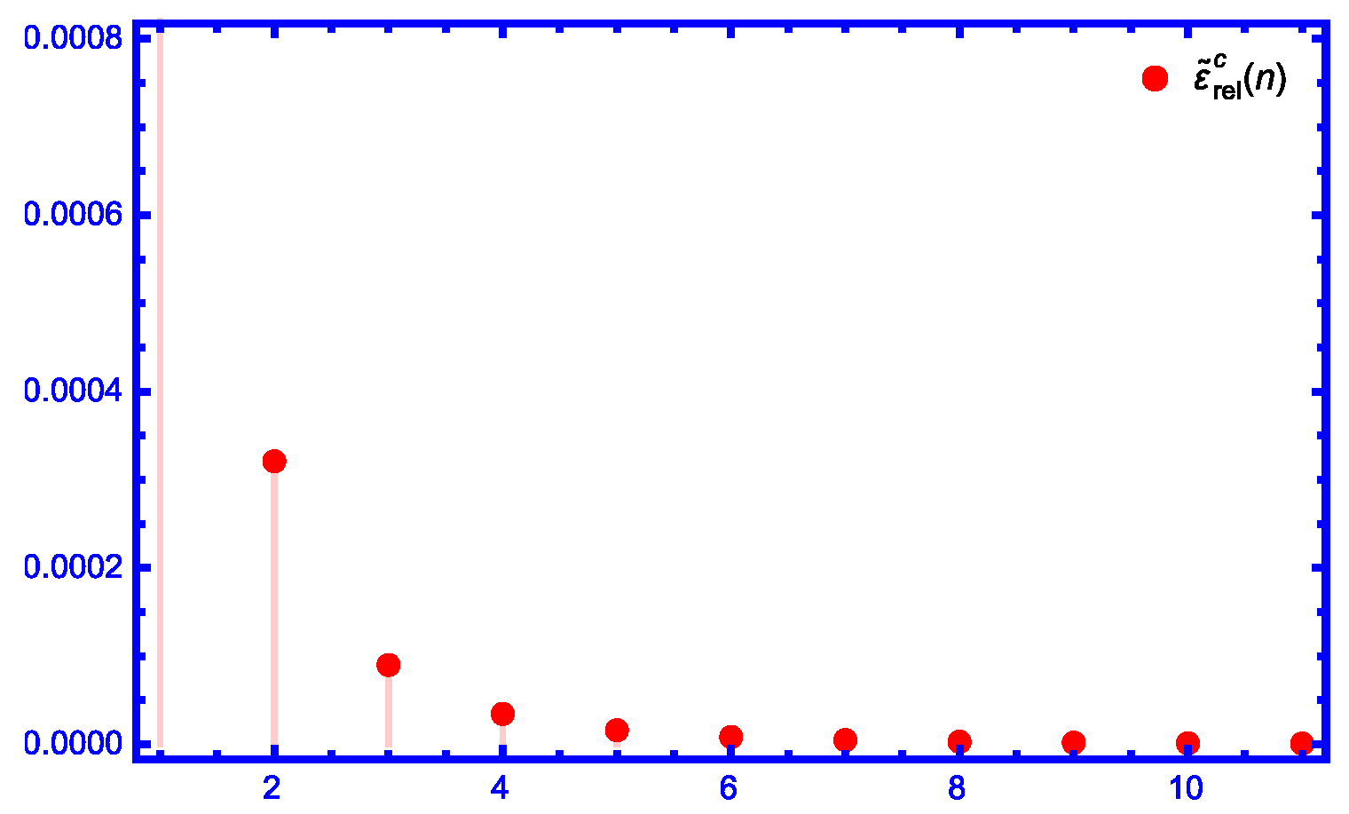
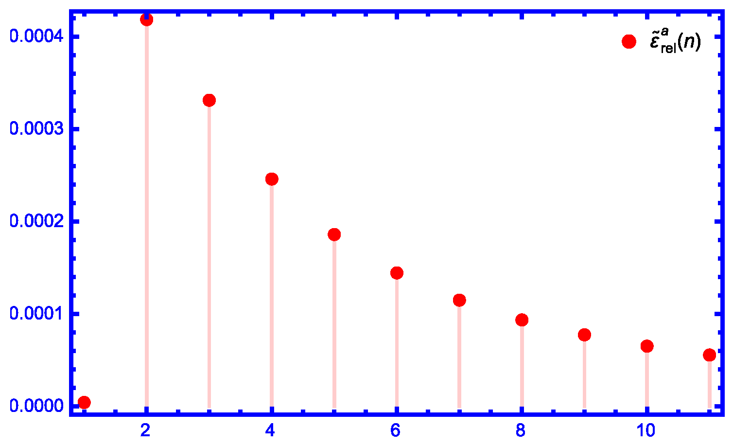
Figure 1. Comparison between the two functions J 2 ( x ) and J ˜ 2 c ( x ) for 0 x 10 .
Axioms 14 00157 g001
Figure 2. The absolute error ε b ( x ) = | J 2 ( x ) J ˜ 2 b ( x ) | for 0 x < 4 .
Axioms 14 00157 g002
Figure 3. The absolute error ε b ( x ) = | J 2 ( x ) J ˜ 2 a ( x ) | for 0 x < 4 .
Axioms 14 00157 g003
Figure 4. Comparison between the two functions J 2 ( x ) and J ˜ 2 b ( x ) for 0 x < 4 .
Axioms 14 00157 g004
Figure 5. Comparison between the two functions J 2 ( x ) and J ˜ 2 a ( x ) for 0 x < 4 .
Axioms 14 00157 g005
Figure 6. The absolute error ε c ( x ) = | J 2 ( x ) J ˜ 2 c ( x ) | for 4 x 15 .
Axioms 14 00157 g006
Figure 7. The absolute error ε a ( x ) = | J 2 ( x ) J ˜ 2 a ( x ) | for 4 x 15 .
Axioms 14 00157 g007
Figure 8. The absolute error ε c ( x ) = | J 2 ( x ) J ˜ 2 c ( x ) | for 15 x 33 .
Axioms 14 00157 g008
Figure 9. The absolute error ε a ( x ) = | J 2 ( x ) J ˜ 2 a ( x ) | for 15 x 33 .
Axioms 14 00157 g009
Figure 10. The absolute error ε c ( x ) = | J 2 ( x ) J ˜ 2 c ( x ) | for 33 x 10 3 .
Axioms 14 00157 g010
Figure 11. The absolute error ε a ( x ) = | J 2 ( x ) J ˜ 2 a ( x ) | for 33 x 10 3 .
Axioms 14 00157 g011
Figure 12. Relative error ε ˜ r e l c ( n ) of zeros for i = 1 , 2 , , 11 .
Axioms 14 00157 g012
Figure 13. Relative error ε ˜ r e l a ( n ) of zeros for i = 1 , 2 , , 11 .
Axioms 14 00157 g013
Table 1. The first eleven positive zeros of J 2 ( x ) , J ˜ 2 c ( x ) and J ˜ 2 a ( x ) .
x i x ˜ i c x ˜ i a Relative Error ε ˜ rel c ( n ) Relative Error ε ˜ rel a ( n )
Zeros of J 2 ( x ) Zeros of J ˜ 2 c ( x ) Zeros of J ˜ 2 a ( x ) of Zeros of J ˜ 2 c ( x ) of Zeros of J ˜ 2 a ( x )
x 1 = 5.1356 x ˜ 1 c = 5.1468 x ˜ 1 a = 5.1356 0.00219574 4.2101 × 10 6
x 2 = 8.4172 x ˜ 2 c = 8.4199 x ˜ 2 a = 8.4207 0.0003209980.000418401
x 3 = 11.6198 x ˜ 3 c = 11.6208 x ˜ 3 a = 11.6236 0.00009002920.0003311
x 4 = 14.7959 x ˜ 4 c = 14.7964 x ˜ 4 a = 14.7995 0.00003456150.000245909
x 5 = 17.9598 x ˜ 5 c = 17.9601 x ˜ 5 a = 17.9631 0.00001600770.000185908
x 6 = 21.1169 x ˜ 6 c = 21.1171 x ˜ 6 a = 21.1200 8.40612 × 10 6 0.00014435
x 7 = 24.2701 x ˜ 7 c = 24.2702 x ˜ 7 a = 24.2729 4.83041 × 10 6 0.000114911
x 8 = 27.4205 x ˜ 8 c = 27.4206 x ˜ 8 a = 27.4231 2.97061 × 10 6 0.0000934664
x 9 = 30.5692 x ˜ 9 c = 30.5692 x ˜ 9 a = 30.5715 1.9263 × 10 6 0.0000774272
x 10 = 33.7165 x ˜ 10 c = 33.7165 x ˜ 10 a = 33.7187 1.30342 × 10 6 0.0000651459
x 11 = 36.8628 x ˜ 11 c = 36.8628 x ˜ 11 a = 36.8649 9.13302 × 10 7 0.0000555473
Disclaimer/Publisher’s Note: The statements, opinions and data contained in all publications are solely those of the individual author(s) and contributor(s) and not of MDPI and/or the editor(s). MDPI and/or the editor(s) disclaim responsibility for any injury to people or property resulting from any ideas, methods, instructions or products referred to in the content.

