Convergence Analysis for Cayley Variational Inclusion Problem Involving XOR and XNOR Operations

Abstract

In this article, we introduce and study a generalized Cayley variational inclusion problem incorporating XOR and XNOR operations. We establish an equivalent fixed-point formulation and demonstrate the Lipschitz continuity of the generalized Cayley approximation operator. Furthermore, we analyze the existence and convergence of the proposed problem using an implicit iterative algorithm. The iterative algorithm and numerical results presented in this study significantly enhance previously known findings in this domain. Finally, a numerical result is provided to support our main result and validate the proposed algorithm using MATLAB programming.

1. Introduction

In 1994, Hassouni and Moudafi [1] introduced the concept of variational inclusion, a generalized form of variational inequalities. Since then, variational inclusions have been extensively studied by researchers to address challenges in diverse fields such as finance, economics, transportation, network analysis, engineering and technology.

A further generalization of Wiener–Hopf equations, known as resolvent equations, were introduced by Noor [2]. Various generalized resolvent operators associated with different monotone operators can be found in the literature. Among these, Cayley approximation operators play a significant role in variational analysis, as they are closely related to resolvent operators. These operators have been effectively applied to study wave equations, heat equations, heat flow and coupled linear sound equations.

Additionally, when dealing with two Boolean operands, the XOR operation determines whether they can pass one another or obstruct each other. A practical demonstration of XOR logic can be observed using polarizing filters, such as those found in polarizing sunglasses. If we hold a polarizing filter up to the lenses of these sunglasses and look through both filters in series, light will pass through when the filters are aligned. However, if one filter is rotated by 90 degrees, the combination blocks the light. This process visually demonstrates XOR logic behavior.

The XOR logical operation is a binary operation that takes two Boolean operands and returns true only if the operands differ, yielding a false result when both operands are identical. XOR is commonly employed to test for the simultaneous falsehood of two conditions and is extensively used in cryptography, error detection (producing parity bits) and fault tolerance. Similarly, the XNOR operation compares two input bits and produces one output bit. If the input bits are identical, the result is one; otherwise, it is zero. Like XOR, XNOR is both commutative and associative. These operations are utilized in hardware for generating pseudo-random numbers and are fundamental in digital computing and linear separability applications. For further details on the XOR operation, refer to the resources listed [3,4,5,6,7,8,9].

In this article, we explore a generalized Cayley inclusion problem involving multi-valued operators and the XOR operation, owing to the significance and applications of the previously mentioned concepts. An iterative algorithm is developed based on the fixed-point equation, and we derive results on existence and convergence. This has applications in solving heat, wave and heat flow problems. A numerical result is presented using MATLAB2024b, accompanied by computational tables and convergence graphs for illustration.

2. Elementary Tools

In this paper, we assume that $\breve{E}$ is a real-ordered Hilbert space equipped with norm $\left|\right|.\left|\right|$ and inner product $⟨.,.⟩$. Again, $C\subseteq \breve{E}$ is a closed convex cone, $C\left(\breve{E}\right)$ is the family of nonempty compact subsets of $\breve{E}$, and $2^{\breve{E}}$ represents the set of all nonempty subsets of $C\left(\breve{E}\right)$.

Definition 1 

([10]). Let r and t be two elements in the real-ordered Hilbert space $\breve{E}$. Consider lub $\{r,t\}$ and glb $\{r,t\}$ for the set $\{r,t\}$ to exist, where lub means least upper bound and glb means greatest lower bound for the set $\{r,t\}$. Then, some binary operations are defined as follows:

(i) 

$r\vee t$ = $inf\{r,t\}$;

(ii) 

$r\wedge t=sup\{r,t\}$;

(iii) 

$r\oplus t=(r-t)\vee (r-t)$;

(iv) 

$r\odot t$ = $(r-t)\wedge (t-r)$.

Here, ∨ is the least upper bound or inf for the set $\{r,t\},\wedge$ is the greatest lower bound or $sup$ for the set $\{r,t\},\oplus$ is called an XOR operation and ⊙ is called an XNOR operation.

Definition 2 

([10]). Let r be any element of the set $C_{\breve{E}}$; then, $C_{\breve{E}}$ is said to be a cone which implies $\lambda r\in C_{\breve{E}}$ for every positive scalar λ.

Definition 3 

([11,12]). A cone $C_{\breve{E}}$ is said to be a normal cone if and only if there exists a constant ${\lambda }_{{\Pi }_{\breve{E}}}>0$ such that $0\le r\le t$ implies $\left|\right|r\left|\right|\le {\lambda }_{{\Pi }_{\breve{E}}}\le \left|\right|t\left|\right|$.

Definition 4 

([11,12]). Let r and t be two elements in $\breve{E}$; then, $C_{\breve{E}}$ is called a cone, provided $r\le t$ holds if and only if $r-t\in C_{\breve{E}}$, where r and t are said to be comparable if either $r\le t$ or $t\le r$. The comparable elements are represented by $r\propto t.$

Proposition 1 

([12]). Let ⊕ and ⊙ be the XOR operation and XNOR operation, respectively. Then, the following conditions hold:

(i) 

$r\odot t=0,(r\odot t)=(t\odot r),(r\oplus t)=0,(r\oplus t)=(t\oplus r),(r\odot t)=-(r\oplus t)$;

(ii) 

if $r\propto 0$ then $-r\oplus 0\le r\le r\oplus 0$;

(iii) 

$\left(\lambda r\right)\oplus \left(\lambda t\right)=\left|\lambda \right|(r\oplus t)$;

(iv) 

$0\le r\oplus t,$ if $r\propto t$;

(v) 

if $r\propto t$ then $r\oplus t=0$ if and only if $r=t.$

Proposition 2 

([11]). Let $C_{\breve{E}}$ be a normal cone in $\breve{E}$ with normal constant ${\lambda }_{{\Pi }_{\breve{E}}}>0,$; then, for each $r,t\in \breve{E}$ the following postulate are holds:

(i) 

$\left|\right|0\oplus 0\left|\right|=\left|\right|0\left|\right|=0$;

(ii) 

$\left|\right|r\vee t\left|\right|=\left|\right|r\left|\right|\vee \left|\right|t\left|\right|\le \left|\right|r\left|\right|+\left|\right|t\left|\right|$;

(iii) 

$\left|\right|r\oplus t\left|\right|\le \left|\right|r-t\left|\right|\le {\lambda }_{\Pi }\left|\right|r\oplus t\left|\right|$;

(iv) 

if $r\propto t,$ then $\left|\right|r\oplus t\left|\right|\le \left|\right|r-t\left|\right|.$

Definition 5. 

A single-valued mapping $\breve{A}:\breve{E}\to \breve{E}$ is called Lipchitz-continuous if there exists a constant ${\lambda }_{\breve{A}}>0$ such that

$$\left|\right|\breve{A}\left(r\right)-\breve{A}\left(t\right)\left|\right|\le {\lambda }_{\breve{A}}\left|\right|r-t\left|\right|,\forall r,t\in \breve{E}.$$

Definition 6. 

Let us consider ${\rm Y}:\breve{E}\times \breve{E}\times \breve{E}\to \breve{E}$ as a single-valued mapping and $D:\breve{E}\to 2^{\breve{E}}$ as the multi-valued mapping. Then,

(i) 

Υ is called Lipschitz continuous in the first argument if there exists a constant ${\lambda }_{{{\rm Y}}_1}>0$ and for any ${\mu }_1\in D\left(r\right),{\mu }_2\in D\left(t\right)$ such that

$$\left|\right|{\rm Y}({\mu }_1,.,.)-{\rm Y}({\mu }_2,.,.)\left|\right|\le {\lambda }_{{{\rm Y}}_1}\left|\right|{\mu }_1-{\mu }_2\left|\right|,\forall r,t\in C\left(\breve{E}\right).$$

(ii) 

Υ is called Lipschitz continuous in the second argument if there exists a constant ${\lambda }_{{{\rm Y}}_2}>0$ and for any ${\mu }_1\in D\left(r\right),{\mu }_2\in D\left(t\right)$ such that

$$\left|\right|{\rm Y}(.,{\mu }_1,.)-{\rm Y}(.,{\mu }_2,.)\left|\right|\le {\lambda }_{{{\rm Y}}_2}\left|\right|{\mu }_1-{\mu }_2\left|\right|,\forall r,t\in C\left(\breve{E}\right).$$

(iii) 

Υ is called Lipschitz continuous in the third argument if there exists a constant ${\lambda }_{{{\rm Y}}_3}>0$ and for any ${\mu }_1\in D\left(r\right),{\mu }_2\in D\left(t\right)$ such that

$$\left|\right|{\rm Y}(.,.,{\mu }_1)-{\rm Y}(.,.,{\mu }_2)\left|\right|\le {\lambda }_{{{\rm Y}}_3}\left|\right|{\mu }_1-{\mu }_2\left|\right|,\forall r,t\in C\left(\breve{E}\right).$$

Definition 7. 

Consider a multi-valued mapping $\psi :\breve{E}\to C\left(\breve{E}\right)$ that is said to be $\mathcal{D}$-Lipschitz continuous. Then, there exists a constant ${\lambda }_{{\mathcal{D}}_{\psi }}>0$ such that

$$\mathcal{D}(\psi \left(r\right),\psi \left(t\right))\le {\lambda }_{{\mathcal{D}}_{\psi }}\left|\right|r-t\left|\right|,\forall r,t\in C\left(\breve{E}\right).$$

Definition 8. 

Suppose $D:\breve{E}\to 2^{\breve{E}}$ is a multi-valued mapping and $\breve{A}:\breve{E}\to \breve{E}$ is a single-valued mapping. The resolvent operator $R_{\breve{A},\rho }^D:\breve{E}\to \breve{E}$ is defined as

$$R_{\breve{A},\rho }^D\left(t\right)={[\breve{A}+\rho D]}^{-1}\left(t\right),\forall r,t\in \breve{E}.$$

τ is an identity mapping and $\rho >0$ is a constant.

Definition 9. 

Suppose $D:\breve{E}\to 2^{\breve{E}}$ is a multi-valued mapping and $\breve{A}:\breve{E}\to \breve{E}$ is a single-valued mapping. The Cayley approximation operator $C_{\breve{A},\rho }^D:\breve{E}\to \breve{E}$ is defined as

$$C_{\breve{A},\rho }^D\left(t\right)=\left[2R_{\breve{A},\rho }^D-\breve{A}\right]\left(t\right),\forall r,t\in \breve{E}.$$

τ is an identity mapping and $\rho >0$ is a constant.

Definition 10. 

Let $\breve{A}:\breve{E}\to \breve{E}$ be a single-valued mapping and $D:\breve{E}\to 2^{\breve{E}}$ be a multi-valued mapping. Then,

(i) 

$\breve{A}$ is called strong comparison mapping if $\breve{A}$ is comparison mapping and $\breve{A}\left(r\right)\propto \breve{A}\left(t\right)$ if and only if $r\propto t,\forall r,t\in \breve{E}.$

(ii) 

$\breve{A}$ is called ρ-order non-extended mapping if there exists a constant $\rho >0$ such that

$$\rho (r\oplus t)\le (\breve{A}\left(r\right)\oplus \breve{A}\left(t\right)),\forall r,t\in \breve{E}.$$

(iii) 

$\breve{A}$ is called a comparison mapping if $r\propto t,r\propto \breve{A}\left(r\right)$ and $t\propto \breve{A}\left(t\right),$ such that

$$\breve{A}\left(r\right)\propto \breve{A}\left(t\right),\forall r,t\in \breve{E}.$$

(iv) 

D is called a comparison mapping if any ${\vartheta }_r\in D\left(r\right),r\propto {\vartheta }_r$ and if $r\propto t,$ as well as for any ${\vartheta }_r\in D\left(r\right)$ and ${\vartheta }_t\in D\left(t\right),$ such that

$${\vartheta }_r\propto {\vartheta }_t,\forall r,t\in \breve{E}.$$

(v) 

The comparison mapping D is called an $\alpha -$ non-ordinary difference mapping if ${\vartheta }_r\in D\left(r\right)$ and ${\vartheta }_t\in D\left(t\right)$ such that

$$({\vartheta }_r\oplus {\vartheta }_t)\oplus {\alpha }_{\breve{A}}(r\oplus t)=0,\forall r,t\in \breve{E}.$$

(vi) 

The comparison mapping D is called ρ-ordered rectangular mapping. If there exists a constant $\rho >0,$ then there exists ${\vartheta }_r\in D\left(r\right)$ and ${\vartheta }_t\in D\left(t\right)$ such that

$$⟨({\vartheta }_r\odot {\vartheta }_t)-(r\oplus t)⟩\ge \rho \left|\right|r\oplus {t\left|\right|}^2,\forall r,t\in \breve{E}.$$

(vii) 

D is called a weak comparison mapping if any $r,t\in \breve{E}$ or $r\propto t$ and there exists ${\vartheta }_r\in D\left(r\right),{\vartheta }_t\in D\left(t\right),r\propto {\vartheta }_r,$ and $t\propto {\vartheta }_t$ such that

$${\vartheta }_r\propto {\vartheta }_t,\forall r,t\in \breve{E}.$$

(viii) 

D is called $\rho -$ weak-ordered different mapping if there exists a constant $\rho >0,$ and there exists ${\vartheta }_r\in D\left(r\right)$ and ${\vartheta }_t\in D\left(t\right)$ such that

$$\rho ({\vartheta }_r-{\vartheta }_t)\propto (r-t),\forall r,t\in \breve{E}.$$

(ix) 

A weak comparison mapping D is called $({\alpha }_{\breve{A}},\rho )-$ weak ANODD if it is an ${\alpha }_{\breve{A}}$ weak non-ordinary difference mapping and ρ-order different weak-comparison mapping with respect to $\breve{A}$ and

$$(\breve{A}+\rho D)\breve{E}=\breve{E},\forall \rho >0.$$

Lemma 1. 

Suppose a multi-valued mapping $D:\breve{E}\to 2^{\breve{E}}$ is an ordered $({\alpha }_{\breve{A}},\rho )$-weak ANODD mapping and $\breve{A}:\breve{E}\to \breve{E}$ is called ξ-order non-extended mapping with respect to $\breve{A}$ such that

$$\left|\left|R_{\breve{A},\rho }^D\left(r\right)\oplus R_{\breve{A},\rho }^D\left(t\right)\right|\right|\le R_{\theta }\left|\right|r\oplus t\left|\right|,\forall r,t\in \breve{E}.$$

where $R_{\theta }={\displaystyle \frac{1}{\xi ({\alpha }_{\breve{A}}\rho -1)}},\rho >{\displaystyle \frac{1}{\xi }},$ and ${\alpha }_{\breve{A}}>{\displaystyle \frac{1}{\rho }}.$

Thus, the resolvent operator $R_{\breve{A},\rho }^D$ is Lipschitz-type-continuous.

Proposition 3. 

Suppose $D:\breve{E}\to 2^{\breve{E}}$ is a multi-valued mapping and a single-valued mapping $\breve{A}:\breve{E}\to \breve{E}$ is ${\lambda }_{\breve{A}}$-Lipschitz continuous. Then, the generalized Cayley approximation operator $C_{\breve{A},\rho }^D$ is ${\lambda }_C$- Lipschitz continuous, which provides $r\propto t,\breve{A}\left(r\right)\propto \breve{A}\left(t\right),R_{\breve{A},\rho }^D\left(r\right)\propto R_{\breve{A},\rho }^D\left(t\right)$ and $C_{\breve{A},\rho }^D\left(r\right)\propto C_{\breve{A},\rho }^D\left(t\right)$ such that

$$\left|\left|C_{\breve{A},\rho }^D\left(r\right)\oplus C_{\breve{A},\rho }^D\left(t\right)\right|\right|\le {\lambda }_C\left|\left|r\oplus t\right|\right|,\forall r,t\in \breve{E}.$$

where ${\lambda }_C={\displaystyle \frac{\xi {\lambda }_{\breve{A}}({\alpha }_{\breve{A}}\rho -1)+2}{\xi ({\alpha }_{\breve{A}}\rho -1)}}.$

Proof. 

Using the Lipschitz continuity of $\breve{A}$ and $R_{\breve{A},\rho }^D$, we evaluate

$$\begin{array}{ccc}\hfill \left|\left|C_{\breve{A},\rho }^D\left(r\right)\oplus C_{\breve{A},\rho }^D\left(t\right)\right|\right|& =& \left|\left|[2R_{\breve{A},\rho }^D-\breve{A}]\left(r\right)\oplus [2R_{\breve{A},\rho }^D-\breve{A}]\left(t\right)\right|\right|\hfill \\ & \le & \left|\left|\breve{A}\left(r\right)\oplus \breve{A}\left(t\right)\right|\right|+2\left|\left|R_{\breve{A},\rho }^D\left(r\right)\oplus R_{\breve{A},\rho }^D\left(t\right)\right|\right|\hfill \\ & \le & {\lambda }_{\breve{A}}\left|\right|r\oplus t\left|\right|+{\displaystyle \frac{2}{\xi ({\alpha }_{\breve{A}}\rho -1)}}\left|\right|r\oplus t\left|\right|\hfill \\ & \le & {\displaystyle \frac{\xi {\lambda }_{\breve{A}}({\alpha }_{\breve{A}}\rho -1)+2}{\xi ({\alpha }_{\breve{A}}\rho -1)}}\left|\right|r\oplus t\left|\right|\hfill \\ & =& {\lambda }_C\left|\right|r\oplus t\left|\right|\hfill \end{array}$$

where ${\lambda }_C={\displaystyle \frac{\xi {\lambda }_{\breve{A}}({\alpha }_{\breve{A}}\rho -1)+2}{\xi ({\alpha }_{\breve{A}}\rho -1)}}.$    □

3. Statement of the Cayley Inclusion Problem

Suppose $g,\breve{A},\breve{B}:\breve{E}\to \breve{E}$ are the single-valued mappings and also $D:\breve{E}\to 2^{\breve{E}}$ are the multi-valued mapping; again, let us consider ${\rm Y}:\breve{E}\times \breve{E}\times \breve{E}\to \breve{E}$ to be another mapping and $\psi ,\varphi ,\phi :\breve{E}\to C\left(\breve{E}\right)$ to be the multi-valued mappings. Let $C_{\breve{A},\rho }^D$ be the generalized Cayley approximation operators for any $\rho >0.$

Find $r\in \breve{E},\breve{u}\in \psi \left(r\right),\breve{v}\in \varphi \left(r\right)$ and $\breve{w}\in \phi \left(r\right)$ such that

$$\begin{array}{c}\hfill 0\in C_{\breve{A},\rho }^D\left(\breve{B}\left(r\right)\right)+{\rm Y}(\breve{u},\breve{v},\breve{w})\oplus D\left(g\left(r\right)\right).\end{array}$$

(1)

If $C_{\breve{A},\rho }^D\left(\breve{B}\left(r\right)\right)=0,{\rm Y}(\breve{u},\breve{v},\breve{w})=0$ and $D\left(g\right(r\left)\right)=D\left(r\right)$, then problem (1) reduces to the problem of finding $r\in \breve{E}$ such that

$$\begin{array}{c}\hfill 0\in D\left(r\right)\end{array}$$

which is the fundamental issue involving the XOR operation and the Cayley approximation operator, represented by Rockafellar [13].

4. Fixed-Point Formulation and Iterative Algorithm

In this section, we demonstrate that problem (1) is equivalent to a fixed-point equation.

Lemma 2. 

Let us consider $r\in \breve{E},\breve{u}\in \psi \left(r\right),\breve{v}\in \varphi \left(r\right)$ and $\breve{w}\in \phi \left(r\right)$ to be the solutions of Cayley variational inclusion problem (1) involving an XOR operation and an XNOR operation if and only if the following equation is satisfied:

$$\begin{array}{c}\hfill g\left(r\right)=R_{\breve{A},\rho }^D\left[\breve{A}\left(g\left(r\right)\right)+\rho \left\{{\rm Y}(\breve{u},\breve{v},\breve{w})\odot C_{\breve{A},\rho }^D\left(\breve{B}\left(r\right)\right)\right\}\right].\end{array}$$

(2)

Proof. 

Suppose $r\in \breve{E},\breve{u}\in \psi \left(r\right),\breve{v}\in \varphi \left(r\right)$ and $\breve{w}\in \phi \left(r\right)$ satisfy Equation (2). Then, we have

$$\begin{array}{ccc}\hfill g\left(r\right)& =& R_{\breve{A},\rho }^D\left[\breve{A}\left(g\left(r\right)\right)+\rho \left\{{\rm Y}(\breve{u},\breve{v},\breve{w})\odot C_{\breve{A},\rho }^D\left(\breve{B}\left(r\right)\right)\right\}\right]\hfill \\ & =& {(\breve{A}+\rho D)}^{-1}\left[\breve{A}\left(g\left(r\right)\right)+\rho \left\{{\rm Y}(\breve{u},\breve{v},\breve{w})\odot C_{\breve{A},\rho }^D\left(\breve{B}\left(r\right)\right)\right\}\right]\hfill \\ \hfill (\breve{A}+\rho D)g\left(r\right)& =& \breve{A}\left(g\left(r\right)\right)+\rho \left\{({\rm Y}(\breve{u},\breve{v},\breve{w})\odot C_{\breve{A},\rho }^D\left(\breve{B}\left(r\right)\right)\right\}\hfill \\ & =& \breve{A}\left(g\left(r\right)\right)+\rho \left\{{\rm Y}(\breve{u},\breve{v},\breve{w})\odot C_{\breve{A},\rho }^D\left(\breve{B}\left(r\right)\right)\right\}\hfill \end{array}$$

$$\begin{array}{ccc}\hfill D\left(g\right(r\left)\right)& =& {\rm Y}(\breve{u},\breve{v},\breve{w})\odot C_{\breve{A},\rho }^D\left(\breve{B}\left(r\right)\right)\hfill \\ \hfill {\rm Y}(\breve{u},\breve{v},\breve{w})\odot D\left(g\left(r\right)\right)& =& {\rm Y}(\breve{u},\breve{v},\breve{w})\odot {\rm Y}(\breve{u},\breve{v},\breve{w})\odot C_{\breve{A},\rho }^D\left(\breve{B}\left(r\right)\right)\hfill \\ & =& C_{\breve{A},\rho }^D\left(\breve{B}\left(r\right)\right)\hfill \\ & 0& \in C_{\breve{A},\rho }^D\left(\breve{B}\left(r\right)\right)+{\rm Y}(\breve{u},\breve{v},\breve{w})\oplus D\left(g\left(r\right)\right),\hfill \end{array}$$

which is the required Cayley variational inclusion problem (1). Now, we establish the subsequent algorithm utilizing Lemma 2 to solve the Cayley variational inclusion problem (1).    □

5. Main Result

In this section, we establish an existence and convergence result via Algorithm 1 for the generalized Cayley variational inclusion problem, which incorporates XOR and XNOR operations (1).

Algorithm 1 For every $r_0\in \breve{E},\breve{u}\in \psi \left(r_0\right),\breve{v}\in \varphi \left(r_0\right)$ and $\breve{w}\in \phi \left(r_0\right)$, enumerate the sequence $\left\{r_n\right\},\left\{{\breve{u}}_n\right\},\left\{{\breve{v}}_n\right\}$ and $\left\{{\breve{w}}_n\right\}$ by taking after the iterative algorithm.

$$\begin{array}{c}\hfill g\left(r_{n+1}\right)=(1-\alpha )g\left(r_n\right)+\alpha R_{\breve{A},\rho }^D\left[\breve{A}\left(g\left(r_n\right)\right)+\rho \left\{{\rm Y}({\breve{u}}_n,{\breve{v}}_n,{\breve{w}}_n)\odot C_{\breve{A},\rho }^D\left(\breve{B}\left(r_n\right)\right)\right\}\right].\end{array}$$ (3) Let us consider ${\breve{u}}_{n+1}\in \psi \left(r_{n+1}\right),{\breve{v}}_{n+1}\in \varphi \left(r_{n+1}\right)$ and ${\breve{w}}_{n+1}\in \phi \left(r_{n+1}\right)$ such that $$\begin{array}{c}\hfill \left|\right|{\breve{u}}_n-{\breve{u}}_{n+1}\left|\right|\le \mathcal{D}(\psi \left(r_n\right),\psi \left(r_{n-1}\right)),\end{array}$$ (4) $$\begin{array}{c}\hfill \left|\right|{\breve{v}}_n-{\breve{v}}_{n+1}\left|\right|\le \mathcal{D}(\varphi \left(r_n\right),\varphi \left(r_{n-1}\right)),\end{array}$$ (5) $$\begin{array}{c}\hfill \left|\right|{\breve{w}}_n-{\breve{w}}_{n+1}\left|\right|\le \mathcal{D}(\phi \left(r_n\right),\phi \left(r_{n-1}\right)),\end{array}$$ (6) where $0\le \alpha \le 1$ and $\rho >0$ are constants and $n=0,1,2,3,···$

Theorem 1. 

Let $\breve{E}$ be a real-ordered Hilbert space and $C_{\breve{E}}$ be a normal cone in $\breve{E}$. Let us consider $g,\breve{A},\breve{B}:\breve{E}\to \breve{E}$ as Lipschitz continuous mappings with constants ${\lambda }_g>0,{\lambda }_{\breve{A}}>0,$ and ${\lambda }_{\breve{B}}>0,$ respectively. Also, we consider ${\rm Y}:\breve{E}\times \breve{E}\times \breve{E}\to \breve{E}$ to be a Lipschitz continuous mapping with constants ${\lambda }_{{{\rm Y}}_1}>0,{\lambda }_{{{\rm Y}}_2}>0$ and ${\lambda }_{{{\rm Y}}_3}>0,$ respectively, and $D:\breve{E}\to 2^{\breve{E}}$ to be the multi-valued mapping. Let $C_{\breve{A},\rho }^D$ be the generalized Cayley approximation operator with Lipschitz continuous ${\lambda }_C$, let the generalized resolvent operator $R_{\breve{A},\rho }^D$ be $R_{\theta }$ Lipschitz continuous and let $\psi ,\varphi ,\phi :\breve{E}\to C\left(\breve{E}\right)$ be the multi-valued mappings with constants ${\lambda }_{{\mathcal{D}}_{\psi }}>0,{\lambda }_{{\mathcal{D}}_{\varphi }}>0$ and ${\lambda }_{{\mathcal{D}}_{\phi }}>0,$ respectively. $r\propto t,R_{\breve{A},\rho }^D\left(r\right)\propto R_{\breve{A},\rho }^D\left(t\right),C_{\breve{A},\rho }^D\left(\breve{A}\left(r\right)\right)\propto C_{\breve{A},\rho }^D\left(\breve{A}\left(t\right)\right),$ $g\left(r_{n+1}\right)\propto g\left(r_n\right),{\rm Y}({\breve{u}}_n,{\breve{v}}_n,{\breve{w}}_n)\propto {\rm Y}({\breve{u}}_{n-1},{\breve{v}}_{n-1},{\breve{w}}_{n-1})$ and $\breve{A}\left(r\right)\propto \breve{A}\left(t\right)$ for all $r,t\in \breve{E}$, where $\rho >0$ is a constant. Suppose that the following conditions are satisfied:

$$\begin{array}{ccc}\hfill & 0<{\displaystyle \frac{{\lambda }_{{\Pi }_{\breve{E}}}}{{\delta }_g}}\{(1-\alpha ){\lambda }_g+\alpha R_{\theta }{\lambda }_{\breve{A}}{\lambda }_g+\alpha \rho R_{\theta }{\lambda }_C{\lambda }_{\breve{B}}+\alpha \rho R_{\theta }{\lambda }_{{{\rm Y}}_1}{\lambda }_{{\mathcal{D}}_{\psi }}+\alpha \rho R_{\theta }{\lambda }_{{{\rm Y}}_2}{\lambda }_{{\mathcal{D}}_{\varphi }}& \\ & +\alpha \rho R_{\theta }{\lambda }_{{{\rm Y}}_3}{\lambda }_{{\mathcal{D}}_{\phi }}\}<1\end{array}$$

(7)

where $R_{\theta }={\displaystyle \frac{1}{\xi ({\alpha }_{\breve{A}}\rho -1)}},\rho >{\displaystyle \frac{1}{\xi }},{\alpha }_{\breve{A}}>{\displaystyle \frac{1}{\rho }},{\lambda }_C={\displaystyle \frac{\xi {\lambda }_{\breve{A}}({\alpha }_{\breve{A}}\rho -1)+2}{\xi ({\alpha }_{\breve{A}}\rho -1)}},$ $0\le \alpha \le 1,\rho >0$, $n=0,1,2,3,···$ Then, $(r,\breve{u},\breve{v},\breve{w})$ is the solution of the Cayley variational inclusions problem (1) involving an XOR operation and an XNOR operation, and the sequences $\left\{r_n\right\},\left\{{\breve{u}}_n\right\},\left\{{\breve{v}}_n\right\}$ and $\left\{{\breve{w}}_n\right\},$ generated by Algorithm 1, strongly convergence at $r,\breve{u},\breve{v}$ and $\breve{w}$, respectively.

Proof. 

We have

$$\begin{array}{cc}\hfill 0\le g\left(r_{n+1}\right)\oplus g\left(r_n\right)& =\{(1-\alpha )g\left(r_n\right)+\alpha R_{\breve{A},\rho }^D[\breve{A}\left(g\left(r_n\right)\right)+\rho \{{\rm Y}({\breve{u}}_n,{\breve{v}}_n,{\breve{w}}_n)\hfill \\ \hfill & \odot C_{\breve{A},\rho }^D\left(\breve{B}\left(r_n\right)\right)\left\}\right]\}\oplus \{(1-\alpha )g\left(r_{n-1}\right)+\alpha R_{\breve{A},\rho }^D[\breve{A}\left(g\left(r_{n-1}\right)\right)\hfill \\ \hfill & +\rho \left\{{\rm Y}({\breve{u}}_{n-1},{\breve{v}}_{n-1},{\breve{w}}_{n-1})\odot C_{\breve{A},\rho }^D\left(\breve{B}\left(r_{n-1}\right)\right)\right\}\left]\right\}\hfill \\ \hfill & \le (1-\alpha )(g\left(r_n\right)\oplus g\left(r_{n-1}\right))+\alpha \left\{R_{\breve{A},\rho }^D\right[\breve{A}\left(g\left(r_n\right)\right)\hfill \\ \hfill & +\rho \{{\rm Y}({\breve{u}}_n,{\breve{v}}_n,{\breve{w}}_n)\odot C_{\breve{A},\rho }^D\left(\breve{B}\left(r_n\right)\right)\left\}\right]\oplus R_{\breve{A},\rho }^D[\breve{A}\left(g\left(r_{n-1}\right)\right)\hfill \\ \hfill & +\rho \left\{{\rm Y}({\breve{u}}_{n-1},{\breve{v}}_{n-1},{\breve{w}}_{n-1})\odot C_{\breve{A},\rho }^D\left(\breve{B}\left(r_{n-1}\right)\right)\right\}\left]\right\}.\hfill \end{array}$$

(8)

Using (4), (5), (6), (iii) of Proposition 2, and (8), we obtain,

$$\begin{array}{ccc}\hfill \left|\right|g\left(r_{n+1}\right)\oplus g\left(r_n\right)\left|\right|& \le & (1-\alpha ){\lambda }_{{\Pi }_{\breve{E}}}\left|\right|g\left(r_n\right)\oplus g\left(r_{n-1}\right)\left|\right|+\alpha {\lambda }_{{\Pi }_{\breve{E}}}\left|\right|R_{\breve{A},\rho }^D[\breve{A}\left(g\left(r_n\right)\right)\hfill \\ \hfill & & +\rho \{{\rm Y}({\breve{u}}_n,{\breve{v}}_n,{\breve{w}}_n)\odot C_{\breve{A},\rho }^D\left(\breve{B}\left(r_n\right)\right)\}]\oplus R_{\breve{A},\rho }^D[\breve{A}\left(g\left(r_{n-1}\right)\right)\hfill \\ \hfill & & +\rho \{{\rm Y}({\breve{u}}_{n-1},{\breve{v}}_{n-1},{\breve{w}}_{n-1})\odot C_{\breve{A},\rho }^D\left(\breve{B}\left(r_{n-1}\right)\right)\}\left]\right||\hfill \\ \hfill & \le & (1-\alpha ){\lambda }_{{\Pi }_{\breve{E}}}\left|\right|g\left(r_n\right)\oplus g\left(r_{n-1}\right)\left|\right|+\alpha {\lambda }_{{\Pi }_{\breve{E}}}{R}_{\theta }\left|\right|[\breve{A}\left(g\left(r_n\right)\right)\hfill \\ \hfill & & +\rho \{{\rm Y}({\breve{u}}_n,{\breve{v}}_n,{\breve{w}}_n)\odot C_{\breve{A},\rho }^D\left(\breve{B}\left(r_n\right)\right)\}]\oplus [\breve{A}\left(g\left(r_{n-1}\right)\right)\hfill \\ \hfill & & +\rho \{{\rm Y}({\breve{u}}_{n-1},{\breve{v}}_{n-1},{\breve{w}}_{n-1})\odot C_{\breve{A},\rho }^D\left(\breve{B}\left(r_{n-1}\right)\right)\}\left]\right||\hfill \\ \hfill & \le & (1-\alpha ){\lambda }_{{\Pi }_{\breve{E}}}\left|\right|g\left(r_n\right)\oplus g\left(r_{n-1}\right)\left|\right|+\alpha {\lambda }_{{\Pi }_{\breve{E}}}{R}_{\theta }\left|\right|\breve{A}\left(g\left(r_n\right)\right)\hfill \\ \hfill & & \oplus \breve{A}\left(g\left(r_{n-1}\right)\right)\left|\right|+\alpha \rho R_{\theta }{\lambda }_{{\Pi }_{\breve{E}}}\left|\right|{\rm Y}({\breve{u}}_n,{\breve{v}}_n,{\breve{w}}_n)\hfill \\ \hfill & & \oplus {\rm Y}({\breve{u}}_{n-1},{\breve{v}}_{n-1},{\breve{w}}_{n-1})\left|\right|+\alpha \rho R_{\theta }{\lambda }_{{\Pi }_{\breve{E}}}\left|\right|C_{\breve{A},\rho }^D\left(\breve{B}\left(r_n\right)\right)\hfill \\ \hfill & & \oplus C_{\breve{A},\rho }^D\left(\breve{B}\left(r_{n-1}\right)\right)\left|\right|\hfill \\ \hfill & \le & (1-\alpha ){\lambda }_{{\Pi }_{\breve{E}}}{\lambda }_g\left|\right|r_n\oplus r_{n-1}\left|\right|+\alpha {\lambda }_{{\Pi }_{\breve{E}}}{R}_{\theta }{\lambda }_{\breve{A}}\left|\right|g\left(r_n\right)\hfill \\ \hfill & & \oplus g\left(r_{n-1}\right)\left|\right|+\alpha \rho R_{\theta }{\lambda }_{{\Pi }_{\breve{E}}}\left|\right|{\rm Y}({\breve{u}}_n,{\breve{v}}_n,{\breve{w}}_n)\hfill \\ \hfill & & \oplus {\rm Y}({\breve{u}}_{n-1},{\breve{v}}_{n-1},{\breve{w}}_{n-1})\left|\right|+\alpha \rho R_{\theta }{\lambda }_{{\Pi }_{\breve{E}}}{\lambda }_C\left|\right|\breve{B}\left(r_n\right)\oplus \breve{B}\left(r_{n-1}\right)\left|\right|\hfill \\ \hfill & \le & (1-\alpha ){\lambda }_{{\Pi }_{\breve{E}}}{\lambda }_g\left|\right|r_n\oplus r_{n-1}\left|\right|+\alpha {\lambda }_{{\Pi }_{\breve{E}}}{R}_{\theta }{\lambda }_{\breve{A}}{\lambda }_g\left|\right|r_n\hfill \\ \hfill & & \oplus r_{n-1}\left|\right|+\alpha \rho R_{\theta }{\lambda }_{{\Pi }_{\breve{E}}}{\lambda }_C{\lambda }_{\breve{B}}\left|\right|r_n\oplus r_{n-1}\left|\right|\hfill \\ & & +\alpha \rho R_{\theta }{\lambda }_{{\Pi }_{\breve{E}}}\left|\right|{\rm Y}({\breve{u}}_n,{\breve{v}}_n,{\breve{w}}_n)\oplus {\rm Y}({\breve{u}}_{n-1},{\breve{v}}_{n-1},{\breve{w}}_{n-1})\left|\right|.\hfill \end{array}$$

(9)

Now, we have the following from the definition of $\mathcal{D}$-Lipschitz continuity and (i) of Proposition 1.

$$\begin{array}{ccc}\hfill & & \left|\right|{\rm Y}({\breve{u}}_n,{\breve{v}}_n,{\breve{w}}_n)\oplus {\rm Y}({\breve{u}}_{n-1},{\breve{v}}_{n-1},{\breve{w}}_{n-1})\left|\right|\hfill \\ \hfill & =& \left|\right|{\rm Y}({\breve{u}}_n,{\breve{v}}_n,{\breve{w}}_n)\oplus {\rm Y}({\breve{u}}_{n-1},{\breve{v}}_n,{\breve{w}}_n)\oplus {\rm Y}({\breve{u}}_{n-1},{\breve{v}}_n,{\breve{w}}_n)\hfill \\ \hfill & & \oplus {\rm Y}({\breve{u}}_{n-1},{\breve{v}}_{n-1},{\breve{w}}_n)\oplus {\rm Y}({\breve{u}}_{n-1},{\breve{v}}_{n-1},{\breve{w}}_n)\oplus {\rm Y}({\breve{u}}_{n-1},{\breve{v}}_{n-1},{\breve{w}}_{n-1})\left|\right|\hfill \\ \hfill & =& \left|\right|{\rm Y}({\breve{u}}_n,{\breve{v}}_n,{\breve{w}}_n)\oplus {\rm Y}({\breve{u}}_{n-1},{\breve{v}}_n,{\breve{w}}_n)\left|\right|+\left|\right|{\rm Y}({\breve{u}}_{n-1},{\breve{v}}_n,{\breve{w}}_n)\oplus {\rm Y}({\breve{u}}_{n-1},{\breve{v}}_{n-1},{\breve{w}}_n)\left|\right|\hfill \\ \hfill & & +\left|\right|{\rm Y}({\breve{u}}_{n-1},{\breve{v}}_{n-1},{\breve{w}}_n)\oplus {\rm Y}({\breve{u}}_{n-1},{\breve{v}}_{n-1},{\breve{w}}_{n-1})\left|\right|\hfill \\ \hfill & \le & {\lambda }_{{{\rm Y}}_1}\left|\right|{\breve{u}}_n\oplus {\breve{u}}_{n-1}\left|\right|+{\lambda }_{{{\rm Y}}_2}\left|\right|{\breve{v}}_n\oplus {\breve{v}}_{n-1}\left|\right|+{\lambda }_{{{\rm Y}}_3}\left|\right|{\breve{w}}_n\oplus {\breve{w}}_{n-1}\left|\right|\hfill \\ \hfill & \le & {\lambda }_{{{\rm Y}}_1}\mathcal{D}(\psi \left(r_n\right),\psi \left(r_{n-1}\right))+{\lambda }_{{{\rm Y}}_2}\mathcal{D}(\varphi \left(r_n\right),\varphi \left(r_{n-1}\right))+{\lambda }_{{{\rm Y}}_3}\mathcal{D}(\phi \left(r_n\right),\phi \left(r_{n-1}\right))\hfill \\ & \le & {\lambda }_{{{\rm Y}}_1}{\lambda }_{{\mathcal{D}}_{\psi }}\left|\right|r_n\oplus r_{n-1}\left|\right|+{\lambda }_{{{\rm Y}}_2}{\lambda }_{{\mathcal{D}}_{\varphi }}\left|\right|r_n\oplus r_{n-1}\left|\right|+{\lambda }_{{{\rm Y}}_3}{\lambda }_{{\mathcal{D}}_{\phi }}\left|\right|r_n\oplus r_{n-1}\left|\right|.\hfill \end{array}$$

(10)

Combining (9) and (10), we obtain

$$\begin{array}{ccc}\hfill \left|\right|g\left(r_{n+1}\right)\oplus g\left(r_n\right)\left|\right|& \le & (1-\alpha ){\lambda }_{{\Pi }_{\breve{E}}}{\lambda }_g\left|\right|r_n\oplus r_{n-1}\left|\right|+\alpha {\lambda }_{{\Pi }_{\breve{E}}}{R}_{\theta }{\lambda }_{\breve{A}}{\lambda }_g\left|\right|r_n\oplus r_{n-1}\left|\right|\hfill \\ \hfill & & +\alpha \rho R_{\theta }{\lambda }_{{\Pi }_{\breve{E}}}{\lambda }_C{\lambda }_{\breve{B}}\left|\right|r_n\oplus r_{n-1}\left|\right|+\alpha \rho R_{\theta }{\lambda }_{{\Pi }_{\breve{E}}}{\lambda }_{{{\rm Y}}_1}{\lambda }_{{\mathcal{D}}_{\psi }}\left|\right|r_n\hfill \\ \hfill & & \oplus r_{n-1}\left|\right|+\alpha \rho R_{\theta }{\lambda }_{{\Pi }_{\breve{E}}}{\lambda }_{{{\rm Y}}_2}{\lambda }_{{\mathcal{D}}_{\varphi }}\left|\right|r_n\oplus r_{n-1}\left|\right|\hfill \\ \hfill & & +\alpha \rho R_{\theta }{\lambda }_{{\Pi }_{\breve{E}}}{\lambda }_{{{\rm Y}}_3}{\lambda }_{{\mathcal{D}}_{\phi }}\left|\right|r_n\oplus r_{n-1}\left|\right|\hfill \\ \hfill & \le & \{(1-\alpha ){\lambda }_{{\Pi }_{\breve{E}}}{\lambda }_g+\alpha {\lambda }_{{\Pi }_{\breve{E}}}{R}_{\theta }{\lambda }_{\breve{A}}{\lambda }_g+\alpha \rho R_{\theta }{\lambda }_{{\Pi }_{\breve{E}}}{\lambda }_C{\lambda }_{\breve{B}}\hfill \\ \hfill & & +\alpha \rho R_{\theta }{\lambda }_{{\Pi }_{\breve{E}}}{\lambda }_{{{\rm Y}}_1}{\lambda }_{{\mathcal{D}}_{\psi }}+\alpha \rho R_{\theta }{\lambda }_{{\Pi }_{\breve{E}}}{\lambda }_{{{\rm Y}}_2}{\lambda }_{{\mathcal{D}}_{\varphi }}\hfill \\ & & +\alpha \rho R_{\theta }{\lambda }_{{\Pi }_{\breve{E}}}{\lambda }_{{{\rm Y}}_3}{\lambda }_{{\mathcal{D}}_{\phi }}\left\}\right||r_n\oplus r_{n-1}\left|\right|.\hfill \end{array}$$

(11)

Using (iv) of Proposition 2 in (11), we have

$$\begin{array}{ccc}\hfill \left|\right|g\left(r_{n+1}\right)-g\left(r_n\right)\left|\right|& \le & \{(1-\alpha ){\lambda }_{{\Pi }_{\breve{E}}}{\lambda }_g+\alpha {\lambda }_{{\Pi }_{\breve{E}}}{R}_{\theta }{\lambda }_{\breve{A}}{\lambda }_g+\alpha \rho R_{\theta }{\lambda }_{{\Pi }_{\breve{E}}}{\lambda }_C{\lambda }_{\breve{B}}\hfill \\ \hfill & & +\alpha \rho R_{\theta }{\lambda }_{{\Pi }_{\breve{E}}}{\lambda }_{{{\rm Y}}_1}{\lambda }_{{\mathcal{D}}_{\psi }}+\alpha \rho R_{\theta }{\lambda }_{{\Pi }_{\breve{E}}}{\lambda }_{{{\rm Y}}_2}{\lambda }_{{\mathcal{D}}_{\varphi }}\hfill \\ & & +\alpha \rho R_{\theta }{\lambda }_{{\Pi }_{\breve{E}}}{\lambda }_{{{\rm Y}}_3}{\lambda }_{{\mathcal{D}}_{\phi }}\left\}\right||r_n-r_{n-1}\left|\right|.\hfill \end{array}$$

(12)

Since g is strongly monotone, we have

$$\begin{array}{c}\hfill \left|\right|g\left(r_{n+1}\right)-g\left(r_n\right)\left|\right|\ge {\delta }_g\left|\right|r_{n+1}-r_n\left|\right|\end{array}$$

which implies that

$$\begin{array}{c}\hfill \left|\right|r_{n+1}-r_n\left|\right|\le {\displaystyle \frac{1}{{\delta }_g}}\left|\right|g\left(r_{n+1}\right)-g\left(r_n\right)\left|\right|.\end{array}$$

(13)

Now, combining (12) and (13), we obtain

$$\begin{array}{cc}\hfill \left|\right|r_{n+1}-r_n\left|\right|& \le {\displaystyle \frac{1}{{\delta }_g}}\{(1-\alpha ){\lambda }_{{\Pi }_{\breve{E}}}{\lambda }_g+\alpha {\lambda }_{{\Pi }_{\breve{E}}}{R}_{\theta }{\lambda }_{\breve{A}}{\lambda }_g+\alpha \rho R_{\theta }{\lambda }_{{\Pi }_{\breve{E}}}{\lambda }_C{\lambda }_{\breve{B}}+\alpha \rho R_{\theta }{\lambda }_{{\Pi }_{\breve{E}}}{\lambda }_{{{\rm Y}}_1}{\lambda }_{{\mathcal{D}}_{\psi }}\hfill \\ \hfill & +\alpha \rho R_{\theta }{\lambda }_{{\Pi }_{\breve{E}}}{\lambda }_{{{\rm Y}}_2}{\lambda }_{{\mathcal{D}}_{\varphi }}+\alpha \rho R_{\theta }{\lambda }_{{\Pi }_{\breve{E}}}{\lambda }_{{{\rm Y}}_3}{\lambda }_{{\mathcal{D}}_{\phi }}\left\}\right||r_n-r_{n-1}\left|\right|\hfill \\ \hfill & \le {\displaystyle \frac{{\lambda }_{{\Pi }_{\breve{E}}}}{{\delta }_g}}\{(1-\alpha ){\lambda }_g+\alpha R_{\theta }{\lambda }_{\breve{A}}{\lambda }_g+\alpha \rho R_{\theta }{\lambda }_C{\lambda }_{\breve{B}}+\alpha \rho R_{\theta }{\lambda }_{{{\rm Y}}_1}{\lambda }_{{\mathcal{D}}_{\psi }}\hfill \\ \hfill & +\alpha \rho R_{\theta }{\lambda }_{{{\rm Y}}_2}{\lambda }_{{\mathcal{D}}_{\varphi }}+\alpha \rho R_{\theta }{\lambda }_{{{\rm Y}}_3}{\lambda }_{{\mathcal{D}}_{\phi }}\left\}\right||r_n-r_{n-1}\left|\right|\hfill \\ \hfill & \le \mathsf{\Omega }\left(\theta \right)\left|\right|r_n-r_{n-1}\left|\right|,\hfill \end{array}$$

(14)

where

$$\begin{array}{cc}\hfill \mathsf{\Omega }\left(\theta \right)& ={\displaystyle \frac{{\lambda }_{{\Pi }_{\breve{E}}}}{{\delta }_g}}\{(1-\alpha ){\lambda }_g+\alpha R_{\theta }{\lambda }_{\breve{A}}{\lambda }_g+\alpha \rho R_{\theta }{\lambda }_C{\lambda }_{\breve{B}}+\alpha \rho R_{\theta }{\lambda }_{{{\rm Y}}_1}{\lambda }_{{\mathcal{D}}_{\psi }}\hfill \\ \hfill & +\alpha \rho R_{\theta }{\lambda }_{{{\rm Y}}_2}{\lambda }_{{\mathcal{D}}_{\varphi }}+\alpha \rho R_{\theta }{\lambda }_{{{\rm Y}}_3}{\lambda }_{{\mathcal{D}}_{\phi }}\}\hfill \end{array}$$

From condition (7), it is clear that $\mathsf{\Omega }\left(\theta \right)<1,$ where $\mathsf{\Omega }\left(\theta \right)={\displaystyle \frac{{\lambda }_{{\Pi }_{\breve{E}}}}{{\delta }_g}}\{(1-\alpha ){\lambda }_g+\alpha R_{\theta }{\lambda }_{\breve{A}}{\lambda }_g+\alpha \rho R_{\theta }{\lambda }_C{\lambda }_{\breve{B}}+\alpha \rho R_{\theta }{\lambda }_{{{\rm Y}}_1}{\lambda }_{{\mathcal{D}}_{\psi }}+\alpha \rho R_{\theta }{\lambda }_{{{\rm Y}}_2}{\lambda }_{{\mathcal{D}}_{\varphi }}+\alpha \rho R_{\theta }{\lambda }_{{{\rm Y}}_3}{\lambda }_{{\mathcal{D}}_{\phi }}\}$. Consequently, (14) implies that $\left\{r_n\right\}$ is a Cauchy sequence in $\breve{E}$. Thus, there exists $r\in \breve{E}$ such that $r_n\to r$ as $n\to \infty .$

From (4), (5) and (6), we have

$$\begin{array}{c}\hfill \left|\right|{\breve{u}}_n-{\breve{u}}_{n-1}\left|\right|\le \mathcal{D}(\psi \left(r_n\right),\psi \left(r_{n-1}\right))\le {\lambda }_{{\mathcal{D}}_{\psi }}\left|\right|r_n\oplus r\left|\right|\le {\lambda }_{{\mathcal{D}}_{\psi }}\left|\right|r_n-r\left|\right|,\end{array}$$

(15)

$$\begin{array}{c}\hfill \left|\right|{\breve{v}}_n-{\breve{v}}_{n-1}\left|\right|\le \mathcal{D}(\varphi \left(r_n\right),\varphi \left(r_{n-1}\right))\le {\lambda }_{{\mathcal{D}}_{\varphi }}\left|\right|r_n\oplus r\left|\right|\le {\lambda }_{{\mathcal{D}}_{\varphi }}\left|\right|r_n-r\left|\right|,\end{array}$$

(16)

$$\begin{array}{c}\hfill \left|\right|{\breve{w}}_n-{\breve{w}}_{n-1}\left|\right|\le \mathcal{D}(\phi \left(r_n\right),\phi \left(r_{n-1}\right))\le {\lambda }_{{\mathcal{D}}_{\phi }}\left|\right|r_n\oplus r\left|\right|\le {\lambda }_{{\mathcal{D}}_{\phi }}\left|\right|r_n-r\left|\right|.\end{array}$$

(17)

Thus $\left\{{\breve{u}}_n\right\},\left\{{\breve{v}}_n\right\}$ and $\left\{{\breve{w}}_n\right\},$ are also Cauchy sequences in $\breve{E}.$ Therefore, there exists $r\in \breve{E},\breve{u}\in \psi \left(r\right),\breve{v}\in \varphi \left(r\right)$ and $\breve{w}\in \phi \left(r\right)$ such that ${\breve{u}}_n\to \breve{u}$, ${\breve{v}}_n\to \breve{v}$ and ${\breve{w}}_n\to \breve{w}$ as $n\to \infty .$ Next, we show that ${\breve{u}}_n\to \breve{u}\in \psi \left(r\right),{\breve{v}}_n\to \breve{v}\in \varphi \left(r\right)$ and ${\breve{w}}_n\to \breve{w}\in \phi \left(r\right)$ as $n\to \infty .$

Furthermore,

$$\begin{array}{ccc}\hfill d(\breve{u},\psi \left(r\right))& \le & inf\left\{\right||\breve{u}-t||,t\in \psi \left(r\right)\}\hfill \\ \hfill & \le & \left|\right|\breve{u}-{\breve{u}}_n\left|\right|+d({\breve{u}}_n,\psi \left(r\right))\hfill \\ & \le & \left|\right|\breve{u}-{\breve{u}}_n\left|\right|+d(\psi \left(r_n\right),\psi \left(r\right))\hfill \\ & \le & \left|\right|\breve{u}-{\breve{u}}_n\left|\right|+{\lambda }_{{\mathcal{D}}_{\psi }}\left|\right|r_n\oplus r\left|\right|\hfill \\ & \le & \left|\right|\breve{u}-{\breve{u}}_n\left|\right|+{\lambda }_{{\mathcal{D}}_{\psi }}\left|\right|r_n\oplus r\left|\right|\to 0,asn\to \infty .\hfill \end{array}$$

Since $\psi \left(r\right)$ is closed, we have $\breve{u}\in \psi \left(r\right).$ Similarly, we can show that $\breve{v}\in \varphi \left(r\right)$ and $\breve{w}\in \phi \left(r\right)$. Finally, we apply the continuity of $g,\breve{A},\breve{B},{\rm Y},R_{\breve{A},\rho }^D,$ and $C_{\breve{A},\rho }^D$, which implies that

$$\begin{array}{c}\hfill g\left(r\right)=R_{\breve{A},\rho }^D\left[\breve{A}\left(g\left(r\right)\right)+\rho \left\{{\rm Y}(\breve{u},\breve{v},\breve{w})\odot C_{\breve{A},\rho }^D\left(\breve{B}\left(r\right)\right)\right\}\right].\end{array}$$

By Lemma 2, $r\in \breve{E}$ is the solution of the Cayley variational inclusion problem (1), where $\breve{u}\in \psi \left(r\right),\breve{v}\in \varphi \left(r\right)$ and $\breve{w}\in \phi \left(r\right)$. □

6. Numerical Result

To illustrate Theorem 1, we present the following numerical example, implemented using MATLAB 2024b, accompanied by three computation tables and three convergence graphs.

Example 1. 

Suppose $\breve{E}=R$ involving inner product $⟨.,.⟩$ and norm $\left|\right|.\left|\right|$, and $D:\breve{E}\to 2^{\breve{E}}$ is a multi-valued mapping.

(i) 

Again, let us consider $g,\breve{A},\breve{B}:\breve{E}\to \breve{E}$ to be the single-valued mappings, ${\rm Y}:\breve{E}\times \breve{E}\times \breve{E}\to \breve{E}$ to be another single-valued mapping, and $\psi ,\varphi ,\phi :\breve{E}\to C\left(\breve{E}\right)$ to be another multi-valued mapping such that

$$D\left(r\right)=\left\{4r\right\}andg\left(r\right)={\displaystyle \frac{5r}{3}}.$$

Then, for any $r_1,r_2\in \breve{E}$, we have

$$\begin{array}{ccc}\hfill \left|\right|g\left(r_1\right)-g\left(r_2\right)\left|\right|& =& \left|\left|{\displaystyle \frac{5r_1}{3}}-{\displaystyle \frac{5r_2}{3}}\right|\right|\hfill \\ & =& {\displaystyle \frac{5}{3}}\left|\right|r_1-r_2\left|\right|\hfill \\ & \le & 2\left|\right|r_1-r_2\left|\right|.\hfill \end{array}$$

Thus, g is Lipschitz continuous with constant ${\lambda }_g=2$ and

$$\begin{array}{ccc}\hfill \left|\right|g\left(r_1\right)-g\left(r_2\right)\left|\right|& =& \left|\left|{\displaystyle \frac{5}{3}}{r}_1-{\displaystyle \frac{5}{3}}{r}_2\right|\right|\hfill \\ & =& {\displaystyle \frac{5}{3}}\left|\right|r_1-r_2\left|\right|\hfill \\ & \ge & {\displaystyle \frac{4}{3}}\left|\right|r_1-r_2\left|\right|.\hfill \end{array}$$

Similarly, g is strongly monotone with constant ${\delta }_g$ =${\displaystyle \frac{4}{3}}.$

(ii) 

Suppose ${\rm Y}:\breve{E}\times \breve{E}\times \breve{E}\to \breve{E}$ is the single-valued mapping and $\psi ,\varphi ,\phi :\breve{E}\to C\left(\breve{E}\right)$ is the multi-valued mappings such that

$$\psi \left(r\right)=\left\{{\displaystyle \frac{r}{6}}\right\},\varphi \left(r\right)=\left\{{\displaystyle \frac{r}{5}}\right\},\phi \left(r\right)=\left\{{\displaystyle \frac{r}{4}}\right\},and{\rm Y}(\breve{u},\breve{v},\breve{w})=\left\{{\displaystyle \frac{\breve{u}}{2}}+{\displaystyle \frac{\breve{v}}{2}}+{\displaystyle \frac{\breve{w}}{2}}\right\}.$$

Now, we have

$$\begin{array}{ccc}\hfill \mathcal{D}\left(\psi \right(r),\psi (t\left)\right)& =& max\left\{\underset{r\in S\left(r\right)}{sup}d(r,F\left(t\right)),\underset{t\in S\left(t\right)}{sup}d(F\left(r\right),t)\right\}\hfill \\ & \le & max\left\{\left|\left|{\displaystyle \frac{r}{6}}-{\displaystyle \frac{t}{6}}\right|\right|,\left|\left|{\displaystyle \frac{t}{6}}-{\displaystyle \frac{r}{6}}\right|\right|\right\}\hfill \\ & \le & {\displaystyle \frac{1}{6}}max\left\{\right||r-t\left|\right|,\left|\right|t-r\left|\right|\}\hfill \\ & \le & {\displaystyle \frac{1}{5}}max\left|\right|r-t\left|\right|.\hfill \end{array}$$

So, ψ is $\mathcal{D}$-Lipschitz continuous with constant ${\lambda }_{{\mathcal{D}}_{\psi }}={\displaystyle \frac{1}{5}}.$ Similarly, we have to show that ${\lambda }_{{\mathcal{D}}_{\varphi }}={\displaystyle \frac{1}{4}},$ and ${\lambda }_{{\mathcal{D}}_{\phi }}={\displaystyle \frac{1}{3}}.$

Hence, Υ is Lipschitz continuous in three arguments with constant ${\lambda }_{{{\rm Y}}_1}={\lambda }_{{{\rm Y}}_2}={\lambda }_{{{\rm Y}}_3}=1.$ Thus, we obtain

$$\begin{array}{ccc}\hfill {\rm Y}(\breve{u},\breve{v},\breve{w})& =& \left({\displaystyle \frac{r}{12}}+{\displaystyle \frac{r}{10}}+{\displaystyle \frac{r}{8}}\right)\hfill \\ & =& {\displaystyle \frac{37}{120}}r.\hfill \end{array}$$

(iii) 

Suppose $\breve{A},\breve{B}:\breve{E}\to \breve{E}$ is the single-valued mappings; $D:\breve{E}\to 2^{\breve{E}}$ is a multi-valued mapping such that

$$\breve{A}\left(r\right)={\displaystyle \frac{r}{3}}and\breve{B}\left(r\right)={\displaystyle \frac{r}{2}}.$$

Now, we have

$$\begin{array}{ccc}\hfill \left|\right|\breve{A}\left(r_1\right)-\breve{A}\left(r_2\right)\left|\right|& =& \left|\left|{\displaystyle \frac{r_1}{3}}-{\displaystyle \frac{r_2}{3}}\right|\right|\hfill \\ & =& {\displaystyle \frac{1}{3}}\left|\right|r_1-r_2\left|\right|\hfill \\ & \le & {\displaystyle \frac{1}{2}}\left|\right|r_1-r_2\left|\right|.\hfill \end{array}$$

Thus, $\breve{A}$ is Lipschitz continuous with constant ${\lambda }_{\breve{A}}={\displaystyle \frac{1}{2}}$. Similarly, we have to show that $\breve{B}$ is Lipschitz continuous with constant ${\lambda }_{\breve{B}}={\displaystyle \frac{2}{3}}$. In addition, $\breve{A}$ and $\breve{B}$ are ξ-ordered non-extended mappings with constant $\xi =1.$

(iv) 

Suppose $D:\breve{E}\to 2^{\breve{E}}$ is the multi-valued mappings and for every constant $\rho >0$ such that

$$\begin{array}{ccc}\hfill D\left(r\right)& =& \left\{4r\right\}.\hfill \end{array}$$

Now, letting $\rho =1$, it is clear that D is $({\alpha }_{\breve{A}},\rho )$-weak ANODD mapping with ${\alpha }_{\breve{A}}=3$.

(v) 

Now, we calculate the obtained resolvent operators $R_{\breve{A},\rho }^D$ such that

$$\begin{array}{ccc}\hfill R_{\breve{A},\rho }^D\left(r\right)& =& {(\breve{A}+\rho D)}^{-1}\left(r\right)\hfill \\ \hfill & =& {\displaystyle \frac{3r}{13}}.\hfill \end{array}$$

Also, we have

$$\begin{array}{ccc}\hfill \left|\left|R_{\breve{A},\rho }^D\left(r_1\right)\oplus R_{\breve{A},\rho }^D\left(r_2\right)\right|\right|& =& \left|\left|{\displaystyle \frac{3r_1}{13}}\oplus {\displaystyle \frac{3r_2}{13}}\right|\right|\hfill \\ \hfill & =& {\displaystyle \frac{3}{13}}\left|\right|r_1\oplus r_2\left|\right|\hfill \\ \hfill & \le & {\displaystyle \frac{1}{2}}\left|\right|r_1\oplus r_2\left|\right|.\hfill \end{array}$$

Thus, $R_{\breve{A},\rho }^D$ is Lipschitz continuous with constant $R_{\theta }={\displaystyle \frac{1}{2}}$, where $R_{\theta }={\displaystyle \frac{1}{\xi ({\alpha }_{\breve{A}}\rho -1)}},\rho >{\displaystyle \frac{1}{{\alpha }_{\breve{A}}}}.$

(vi) 

Using the values of $R_{\breve{A},\rho }^D$, we obtain the generalized Cayley approximation operator as

$$\begin{array}{ccc}\hfill C_{\breve{A},\rho }^D\left(r\right)& =& \left[2R_{\breve{A},\rho }^D-\breve{A}\right]\left(r\right)\hfill \\ \hfill & =& {\displaystyle \frac{6r}{13}}-{\displaystyle \frac{r}{3}}\hfill \\ \hfill & =& {\displaystyle \frac{5r}{39}}.\hfill \end{array}$$

Now, we have

$$\begin{array}{ccc}\hfill \left|\right|C_{\breve{A},\rho }^D\left(r_1\right)\oplus C_{\breve{A},\rho }^D\left(r_2\right)\left|\right|& =& \left|\left|{\displaystyle \frac{5r_1}{39}}\oplus {\displaystyle \frac{5r_2}{39}}\right|\right|\hfill \\ & =& {\displaystyle \frac{5}{39}}\left|\right|r_1\oplus r_2\left|\right|\hfill \\ & \le & {\displaystyle \frac{3}{2}}\left|\right|r_1\oplus r_2\left|\right|.\hfill \end{array}$$

Thus, $C_{\breve{A},\rho }^D$ is Lipschitz continuous with constant ${\lambda }_C={\displaystyle \frac{3}{2}}$ where ${\lambda }_C={\displaystyle \frac{\xi {\lambda }_{\breve{A}}({\alpha }_{\breve{A}}\rho -1)+2}{\xi ({\alpha }_{\breve{A}}\rho -1)}}.$

(vii) 

Now, we consider the interval $0\le {\displaystyle \frac{1}{10}}\le r\le t\le 1$ and ${\lambda }_{{\Pi }_{\breve{E}}}={\displaystyle \frac{1}{2}}$.

(viii) 

Considering the constants calculated above, condition (7) of Theorem 1 is satisfied.

(ix) 

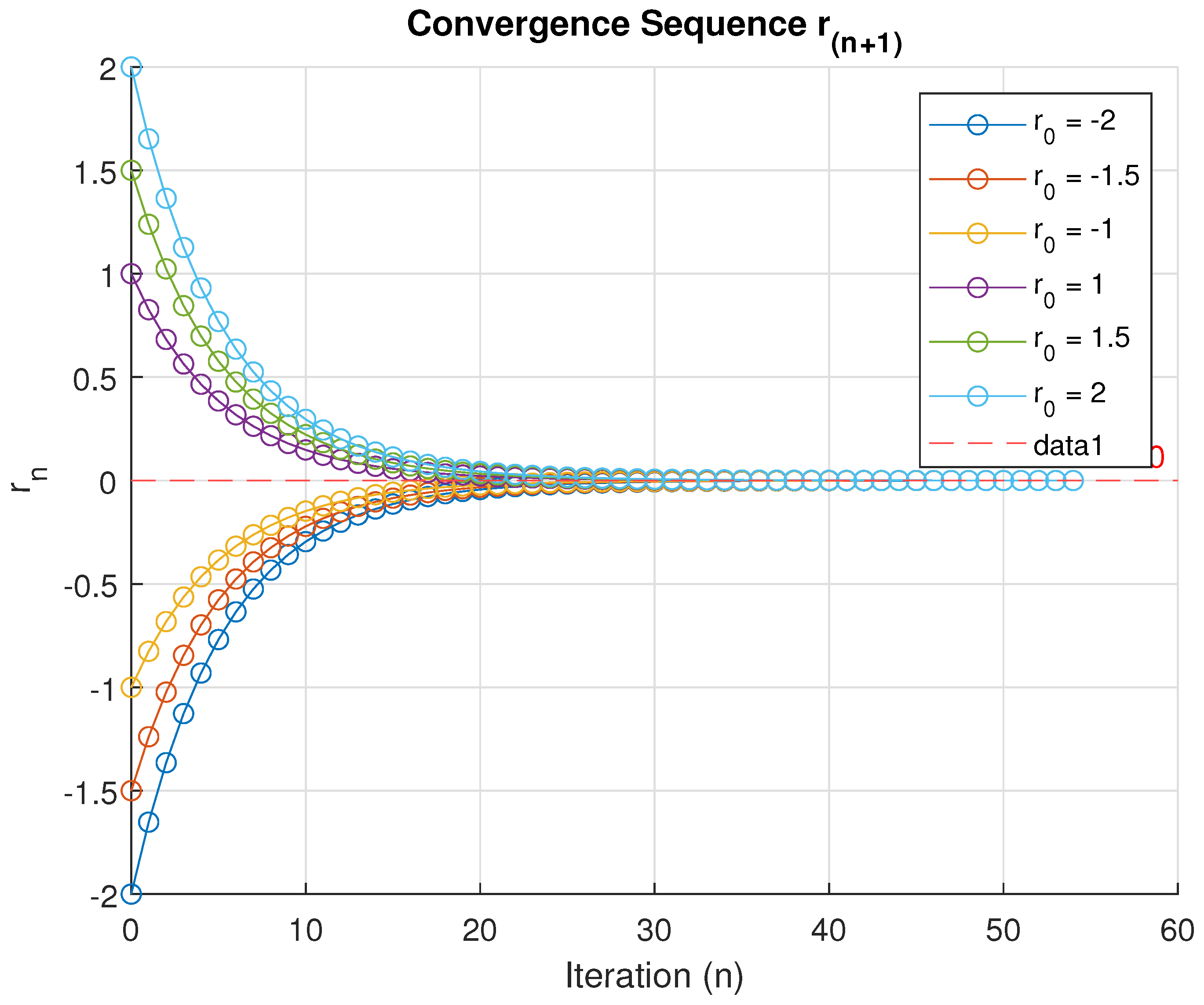
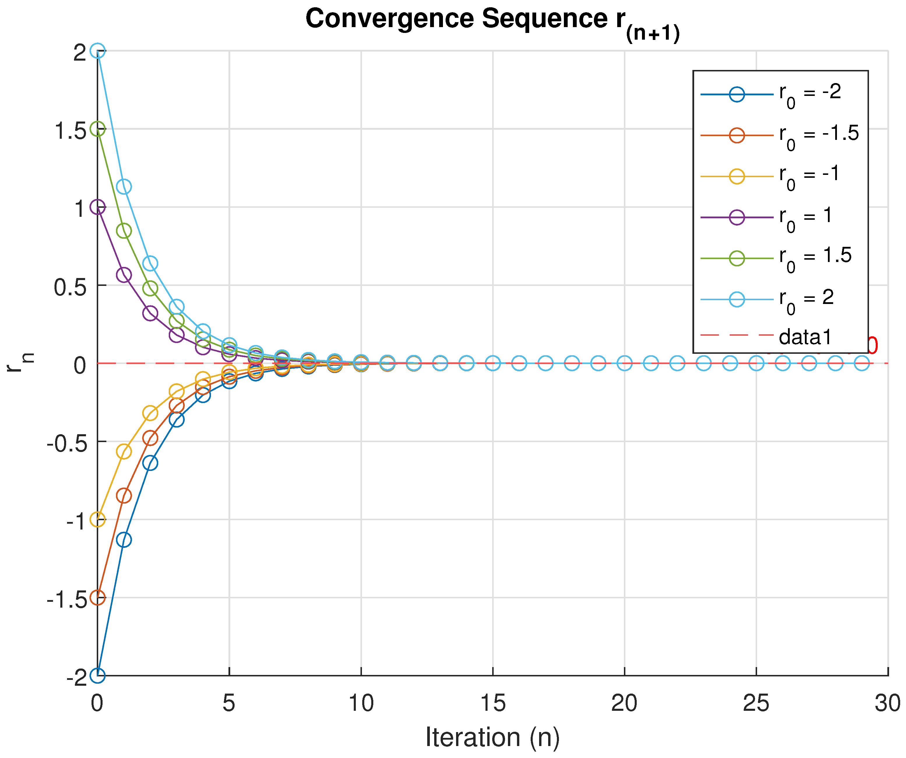
Now putting all values in Equation (3), we obtain

$$\begin{array}{ccc}\hfill g\left(r_{n+1}\right)& =& (1-\alpha )g\left(r_n\right)+\alpha R_{\breve{A},\rho }^D\left[\breve{A}\left(g\left(r_n\right)\right)+\rho \left\{{\rm Y}({\breve{u}}_n,{\breve{v}}_n,{\breve{w}}_n)\odot C_{\breve{A},\rho }^D\left(\breve{B}\left(r_n\right)\right)\right\}\right]\hfill \\ \hfill r_{n+1}& =& (1-\alpha )r_n+{\displaystyle \frac{78174}{608400}}\alpha r_n=(1-0.87\alpha )r_n.\hfill \end{array}$$

In this numerical result, we consider three cases for the composition of the computation table and convergence graph we use the tools of MATLAB-R2024b with some different initial values of $r_0$ and the value of constant α, where $0\le \alpha \le 1$.

In the first case, Consider $\alpha ={\displaystyle \frac{1}{5}}$, and various initial values $r_0=-2,-1.5,-1,1,1.5,2.$ We obtain an excellent graph of the convergence sequence $\left\{r_{n+1}\right\}$ which converges at $r=0$ (after fifty-one iterations), which is the solution of the Cayley variational inclusion problem (1). It is shown through a computation table (Table 1) and convergence graph (Figure 1).

Table 1. The values of the convergent sequence $\left\{r_n\right\}$ with initial values $r_0=-2,-1.5,-1,1,1.5,2$.

No. of Iterations	${\mathit{r}}_0=-2$	${\mathit{r}}_0=-1.5$	${\mathit{r}}_0=-1$	${\mathit{r}}_0=1$	${\mathit{r}}_0=1.5$	${\mathit{r}}_0=2$
n = 1	−1.65200	−1.23900	−0.82600	0.82600	1.23900	1.65200
n = 2	−1.36460	−1.02340	−0.68220	0.68220	1.02340	1.36460
n = 3	−1.12710	−0.84534	−0.56356	0.56356	0.84534	1.12710
n = 4	−0.93100	−0.69825	−0.46550	0.46550	0.69825	0.93100
n = 5	−0.76901	−0.57676	−0.38450	0.38450	0.57676	0.76901
n = 6	−0.63520	−0.47640	−0.31760	0.31760	0.47640	0.63520
n = 15	−0.11369	−0.08526	−0.05684	0.05684	0.08526	0.11369
n = 20	−0.04371	−0.03278	−0.02185	0.02185	0.03278	0.04371
n = 25	−0.01680	−0.01260	−0.00840	0.00840	0.01260	0.01680
n = 35	−0.00248	−0.00186	−0.00124	0.00124	0.00186	0.00248
n = 51	−0.00011	−0.00000	−0.00000	0.00000	0.00000	0.00011
n = 55	−0.00000	−0.00000	−0.00000	0.00000	0.00000	0.00000

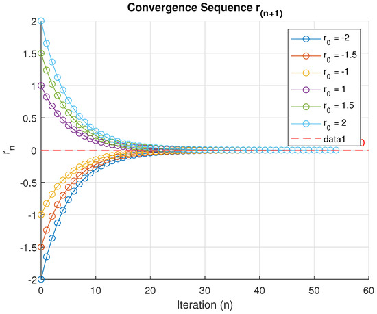Figure 1. Graphical representation of a convergence sequence of {$r_{n+1}$} with different initial values. when $\alpha ={\displaystyle \frac{1}{5}}$.

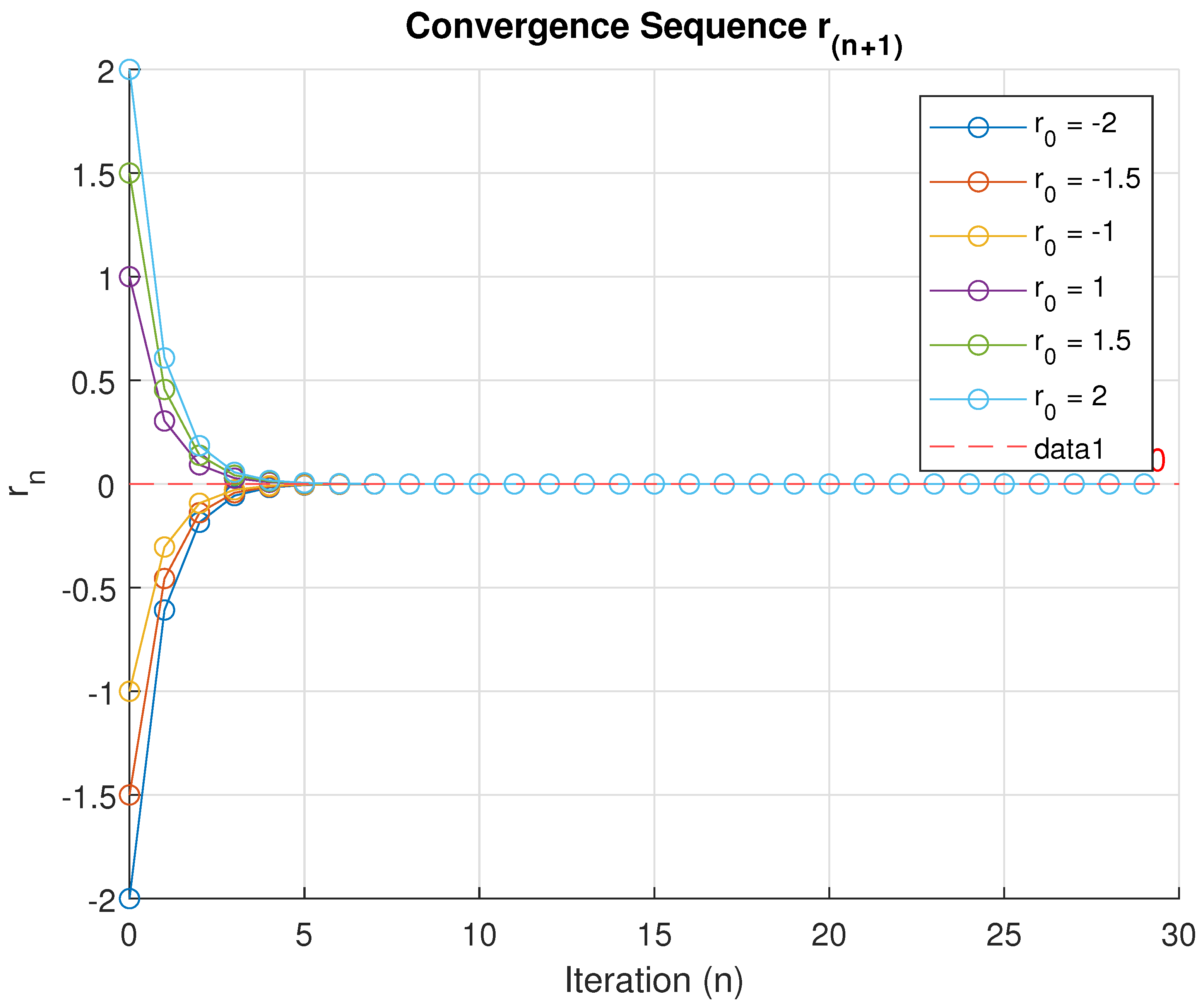
In the second case, Suppose $\alpha ={\displaystyle \frac{1}{2}}$, and the same initial values. We get a computation table (Table 2) and a graph (Figure 2) of the convergence sequence $\left\{r_{n+1}\right\}$ which converges at $r=0$ (after eighteen iterations), which is the solution of the Cayley variational inclusion problem (1).

Table 2. The values of the convergent sequence $\left\{r_n\right\}$ with initial values $r_0=-2,-1.5,-1,1,1.5,2$.

No. of Iterations	${\mathit{r}}_0=-2$	${\mathit{r}}_0=-1.5$	${\mathit{r}}_0=-1$	${\mathit{r}}_0=1$	${\mathit{r}}_0=1.5$	${\mathit{r}}_0=2$
n = 1	−1.13000	−0.84750	−0.56500	0.56500	0.84750	1.13000
n = 2	−0.63845	−0.47884	−0.31922	0.31922	0.47884	0.63845
n = 3	−0.36072	−0.27054	−0.18036	0.18036	0.27054	0.36072
n = 4	−0.20381	−0.15286	−0.10190	0.10190	0.15286	0.20381
n = 5	−0.11515	−0.08636	−0.05757	0.05757	0.08636	0.11515
n = 6	−0.06506	−0.04879	−0.03253	0.03253	0.04879	0.06506
n = 7	−0.03675	−0.02757	−0.01838	0.01838	0.02757	0.03675
n = 11	−0.00663	−0.00497	−0.00331	0.00331	0.00497	0.00663
n = 14	−0.00119	−0.00089	−0.00059	0.00059	0.00089	0.00119
n = 17	−0.00021	−0.00016	−0.00010	0.00010	0.00016	0.00021
n = 18	−0.00012	−0.00000	−0.00000	0.00000	0.00000	0.00012
n = 19	−0.00000	−0.00000	−0.00000	0.00000	0.00000	0.00000
n = 30	−0.00000	−0.00000	−0.00000	0.00000	0.00000	0.00000

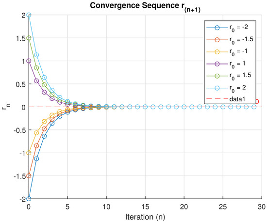
Figure 2. Graphical representation of a convergence sequence of {$r_{n+1}$} with different initial values. when $\alpha ={\displaystyle \frac{1}{2}}$.

In the third case, Suppose $\alpha ={\displaystyle \frac{4}{5}}$, and the same initial values. We get a another computation table (Table 3) and a graph (Figure 3) of the convergence sequence $\left\{r_{n+1}\right\}$ which converges at $r=0$ (after eight iterations), which is the solution of the Cayley variational inclusion problem (1).

Table 3. The values of the convergent sequence $\left\{r_n\right\}$ with initial values $r_0=-2,-1.5,-1,1,1.5,2$.

No. of Iterations	${\mathit{r}}_0=-2$	${\mathit{r}}_0=-1.5$	${\mathit{r}}_0=-1$	${\mathit{r}}_0=1$	${\mathit{r}}_0=1.5$	${\mathit{r}}_0=2$
n = 1	−0.60800	−0.45600	−0.30400	0.30400	0.45600	0.60800
n = 2	−0.18483	−0.13862	−0.09241	0.09241	0.13862	0.18483
n = 3	−0.05618	−0.04214	−0.02809	0.02809	0.04214	0.05618
n = 4	−0.01708	−0.01281	−0.00854	0.00854	0.01281	0.01708
n = 5	−0.00519	−0.00389	−0.00259	0.00259	0.00389	0.00519
n = 6	−0.00157	−0.00118	−0.00078	0.00078	0.00118	0.00157
n = 7	−0.00047	−0.00035	−0.00023	0.00023	0.00035	0.00047
n = 8	−0.00014	−0.00010	−0.00000	0.00000	0.00010	0.00014
n = 9	−0.00000	−0.00000	−0.00000	0.00000	0.00000	0.00000
n = 10	−0.00000	−0.00000	−0.00000	0.00000	0.00000	0.00000
n = 15	−0.00000	−0.00000	−0.00000	0.00000	0.00000	0.00000
n = 20	−0.00000	−0.00000	−0.00000	0.00000	0.00000	0.00000
n = 30	−0.00000	−0.00000	−0.00000	0.00000	0.00000	0.00000

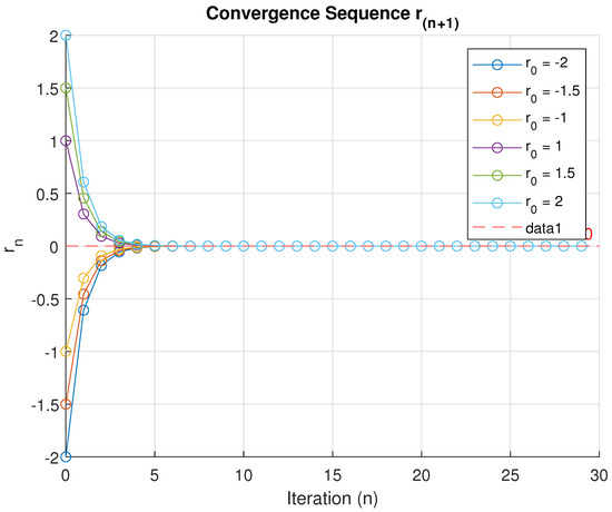
Figure 3. Graphical representation of a convergence sequence $\left\{r_{n+1}\right\}$ with different initial values when $\alpha ={\displaystyle \frac{4}{5}}$.

7. Conclusions

In the draft, we explored a generalized Cayley variational inclusion problem incorporating XOR and XNOR operations in a real-ordered Hilbert space. We analyzed the existence of solutions for the proposed problem using a fixed-point formulation. The proposed algorithms efficiently address generalized Cayley inclusions and solve equations involving XOR and XNOR operations. Furthermore, a numerical result is provided to support our main result and validate the proposed algorithm using MATLAB programming, demonstrating the rapid convergence of the mathematical model and its effectiveness in achieving optimal solutions. From the above Figure 1, Figure 2 and Figure 3, we notice that the sequence $r_{n+1}$ converges to $r=0$. In Figure 1, this occurs within fifty-one iterations, when $\alpha ={\displaystyle \frac{1}{5}}$; in Figure 2, within eighteen iterations, when $\alpha ={\displaystyle \frac{1}{2}}$; and in Figure 3, in eight iterations, when $\alpha ={\displaystyle \frac{4}{5}}$. This pattern indicates that as the value of $\alpha$ increases within the range $0\le \alpha \le 1$, the convergence rate accelerates.

References

- Hassouni, A.; Moudafi, A. A perturbed algorithm for variational inclusions. J. Math. Anal. Appl. 1994, 185, 706–712. [Google Scholar] [CrossRef]
- Noor, M.A. Generalized set-valued variational inclusions and resolvent equations. J. Math. Anal. Appl. 1998, 228, 206–220. [Google Scholar] [CrossRef]
- Ahmad, I.; Irfan, S.S.; Farid, M.; Shukla, P. Nonlinear ordered variational inclusion problem involving XOR operation with fuzzy mappings. J. Inequal. Appl. 2020, 2020, 36. [Google Scholar] [CrossRef]
- Ahmad, I.; Pang, C.T.; Ahmad, R.; Ishtyak, M. System of Yosida inclusions involving XOR-operation. J. Nonlinear Convex Anal. 2017, 18, 831–845. [Google Scholar]
- Ayaka, M.; Tomomi, Y. Applications of the Hille—Yosida theorem to the linearized equations of coupled sound and heat flow. AIMS Math. 2016, 1, 165–177. [Google Scholar] [CrossRef]
- Chang, S.S. Set-valued variational inclusions in Banach spaces. J. Math. Anal. Appl. 2000, 248, 438–454. [Google Scholar] [CrossRef]
- Chang, S.; Yao, J.C.; Wang, L.; Liu, M.; Zhao, L. On the inertial forward-backward splitting technique for solving a system of inclusion problems in Hilbert spaces. Optimization 2021, 70, 2511–2525. [Google Scholar] [CrossRef]
- Yosida, K. Functional Analysis, Grundlehren der Mathematischen Wissenschaften; Springer: New York, NY, USA, 1971. [Google Scholar]
- Iqbal, J.; Rajpoot, A.K.; Islam, M.; Ahmad, R.; Wang, Y. System of Generalized Variational Inclusions Involving Cayley Operators and XOR-Operation in q-Uniformly Smooth Banach Spaces. Mathematics 2022, 10, 2837. [Google Scholar] [CrossRef]
- Khan, A.A.; Tammer, M.; Zalinescu, C. Set-Valued Optimization: An Introduction with Applications; Springer: New York, NY, USA, 2015. [Google Scholar]
- Iqbal, J.; Wang, Y.; Rajpoot, A.K.; Ahmad, R. Generalized Yosida inclusion problem involving multi-valued operator with XOR operation. Demonstr. Math. 2024, 57, 20240011. [Google Scholar] [CrossRef]
- Ali, I.; Ahmad, R.; Wen, C.F. Cayley Inclusion Problem Involving XOR-Operation. Mathematics 2019, 7, 302. [Google Scholar] [CrossRef]
- Rockafellar, R. Monotone Operators and the Proximal Point Algorithm. Siam J. Cont. Optim. 1976, 14, 877–898. [Google Scholar] [CrossRef]
Disclaimer/Publisher’s Note: The statements, opinions and data contained in all publications are solely those of the individual author(s) and contributor(s) and not of MDPI and/or the editor(s). MDPI and/or the editor(s) disclaim responsibility for any injury to people or property resulting from any ideas, methods, instructions or products referred to in the content. |
© 2025 by the authors. Licensee MDPI, Basel, Switzerland. This article is an open access article distributed under the terms and conditions of the Creative Commons Attribution (CC BY) license (https://creativecommons.org/licenses/by/4.0/).