Enumerating the Number of Spanning Trees of Pyramid Graphs Based on Some Nonahedral Graphs

Abstract

The enumeration of spanning trees in various graph forms has been made easier by the study of electrically equivalent transformations, which was motivated by Kirchhoff’s work on electrical networks. In this work, using knowledge of difference equations, the electrically equivalent transformations and rules of weighted generating function are used to calculate the explicit formulas of the number of spanning trees of novel pyramid graph types based on some nonahedral graphs. Lastly, we compare our graphs’ entropy with that of other average-degree graphs that have been researched.

1. Introduction

Finding closed-form formulations for the complexity (number of spanning trees) in different graph types has attracted a lot of attention. Important applications of this field of study include counting Eulerian circuits [1,2], expanding network analysis techniques in psychological networks [3], enumerating chemical isomers [4,5], and tackling intractable problems such as the traveling salesman and Steiner tree problems [6]. Finding the most complex graphs can also be accomplished by looking at different kinds of graphs, which has uses in network resilience [7,8].

Because all nodes in a network represented by a graph must be able to communicate with one another, the graph must have a spanning tree. By increasing the number of spanning trees, dependability can be increased.

For a connected graph $G=(V,E)$ with $n$ vertices, the number of spanning trees can be found using a Kirchhoff classical result [9] from 1847. The Kirchhoff matrix is a characteristic matrix $L=D-A$, where $A$ is the adjacency matrix of $G$, and $D$is the diagonal matrix of the degrees of $G$. The total number of spanning trees in graph $G$ is equal to all of $L$’s co-factors, $L=[a_{ij}]$ defined as follows:

$$L=[a_{ij}]=\left\{\begin{array}{l}\mathit{deg}(v_i) \mathrm{i}\mathrm{f} i=j\\ -1 \mathrm{i}\mathrm{f} (v_i,v_j)\in E\left(G\right)\\ 0 \mathrm{i}\mathrm{f} (v_i,v_j)\notin E\left(G\right)\end{array}\right.$$

In other words, the off-diagonal components are $-1$ for those that are present if an edge connects the two vertices and $0$ otherwise, and the diagonal elements have values equal to the degree of the associated vertices. Many attempts have been made to count the complexity of some specialized graphs using various methodologies, but for a large generic graph, assessing the appropriate determinant is laborious and computationally unfeasible.

An additional approach to computation is as follows. Let indicate the matrix’s eigenvalues of a graph with vertices. Kelmans and Chelnokov [10] demonstrated in 1974 that

$$\tau (G)={\displaystyle \frac{1}{n}}{\displaystyle \prod _{i=1}^{n-1}{\mu }_i}.$$

(1)

The deletion–contraction approach is a popular technique for determining the number of spanning tresses. The number of spanning trees $\tau \left(G\right)$ in a multigraph $G$ can be determined using this reliable method. This method uses the fact that

$$\tau \left(G\right)=\tau (G-e)+\tau (G/e)$$

(2)

where $G-e$ denotes the graph obtained by deleting an arbitrary edge $e$, and $G/e$ denotes the graph obtained by contracting an arbitrary edge $e$ [11,12]. A number of methods have been developed to determine the number of spanning trees of certain graphs; some of these methods are given in [13,14,15,16,17].

Kirchhoff was inspired to study electrical networks because an edge-weighted graph, whose weights indicate the conductance of the corresponding edges, may be viewed as an electrical network. The effect conductance between two vertices $u \mathrm{a}\mathrm{n}\mathrm{d} v$ can be expressed as the quotient of the (weighted) number of spanning trees and the (weighted) number of so-called thickets, which are spanning forests with exactly two components and the property that each component contains precisely one of the vertices $u \mathrm{a}\mathrm{n}\mathrm{d} v$ [18,19,20,21]. The impact of a few basic modifications on the quantity of spanning trees is listed below. The weighted number of spanning trees $G$ is indicated by $\tau \left(G\right)$ and let $G$ be an edge weighted graph and $H$ be the associated electrically equivalent graph.

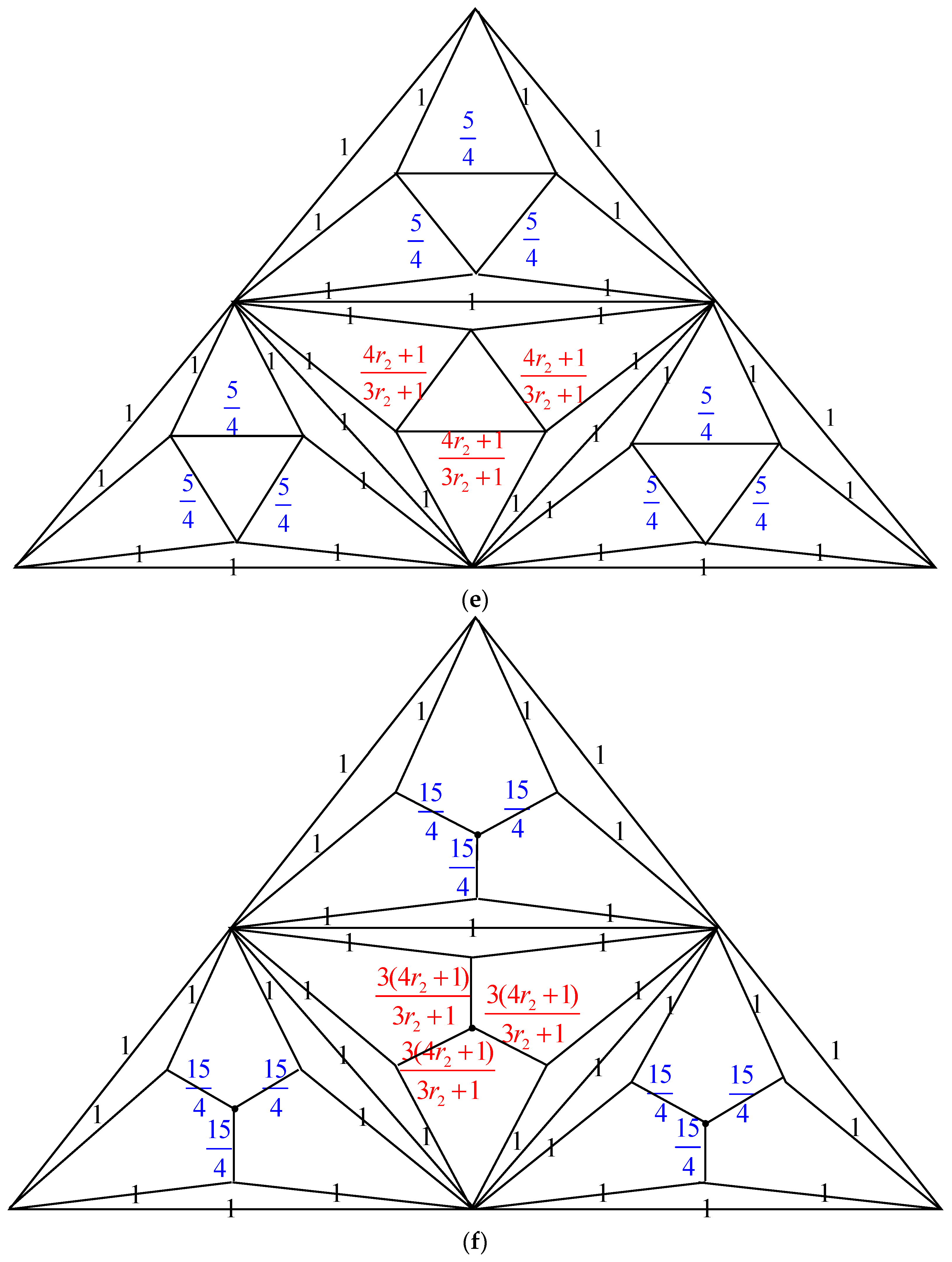
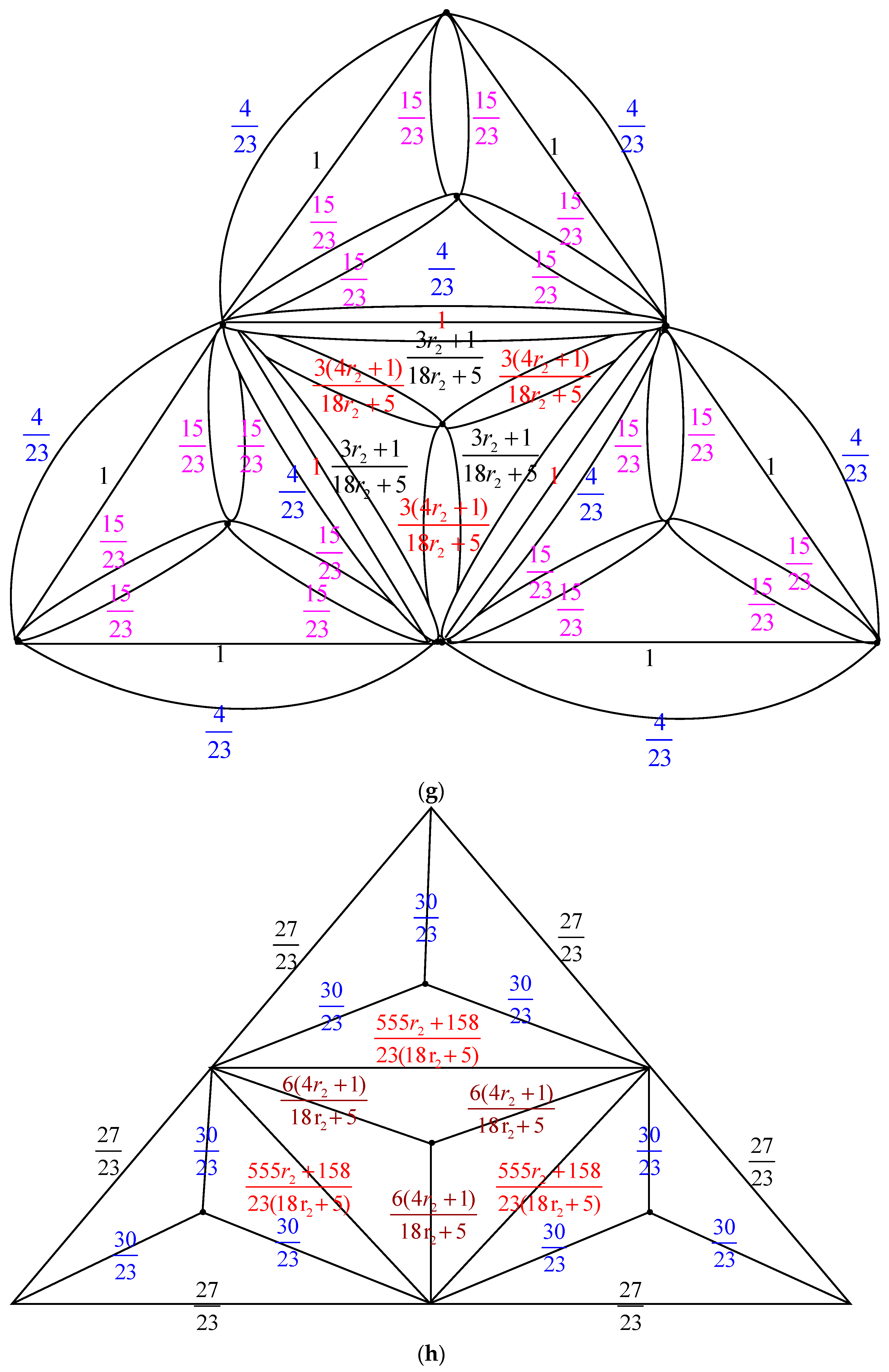
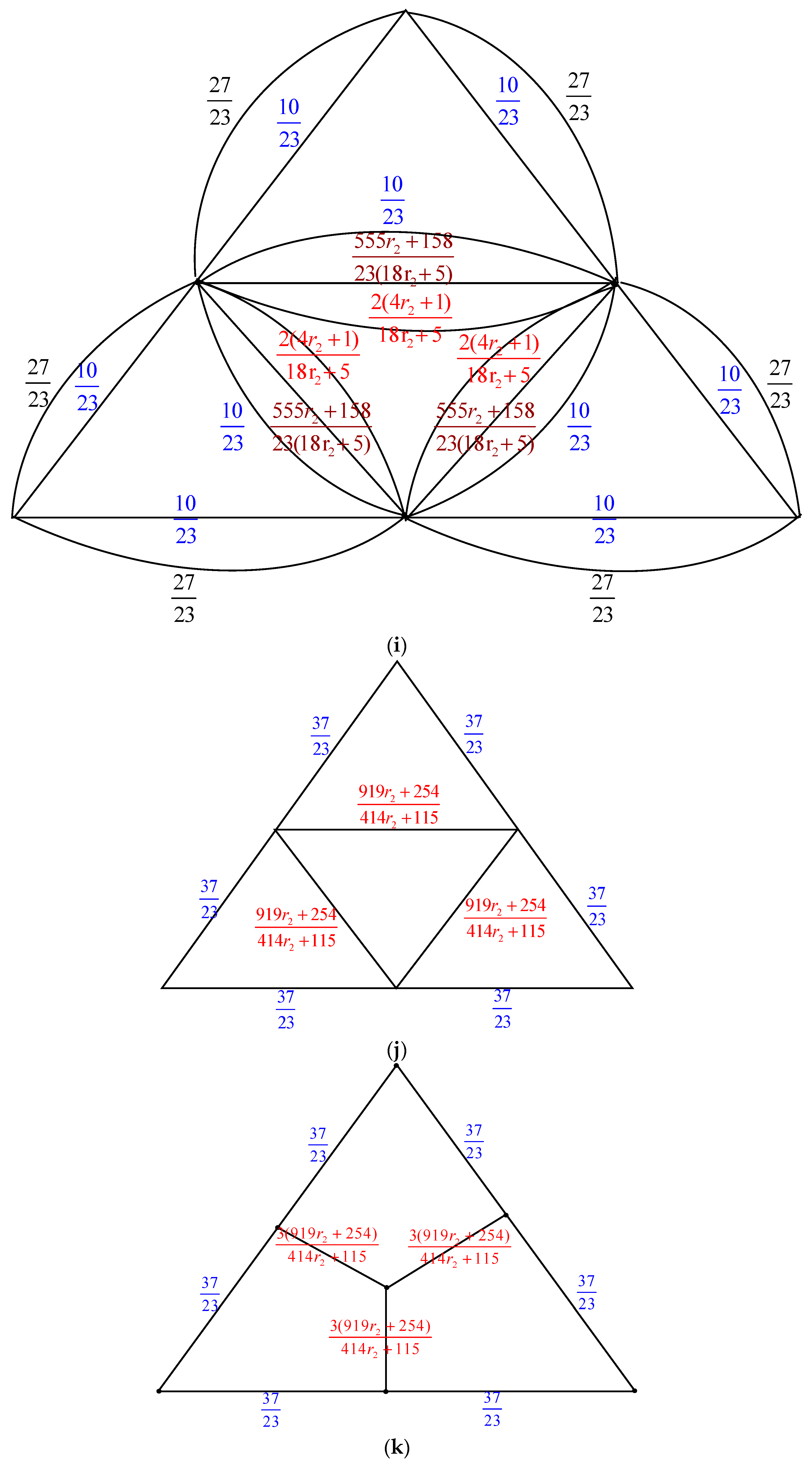
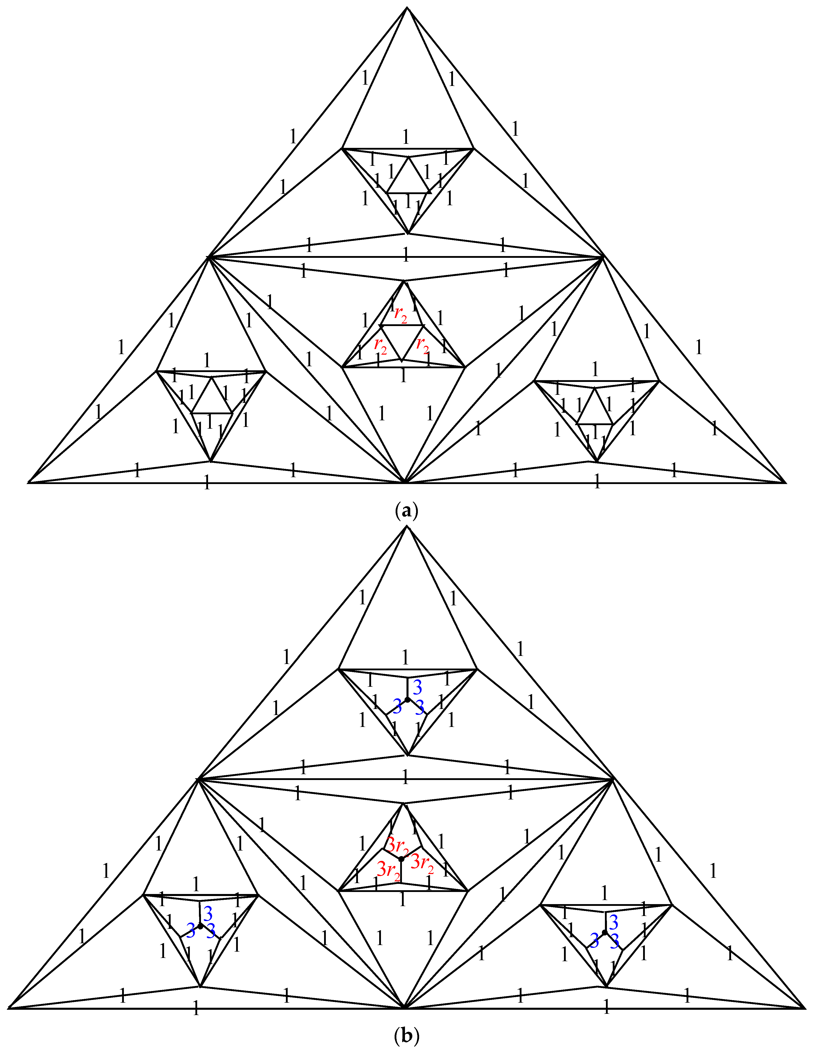
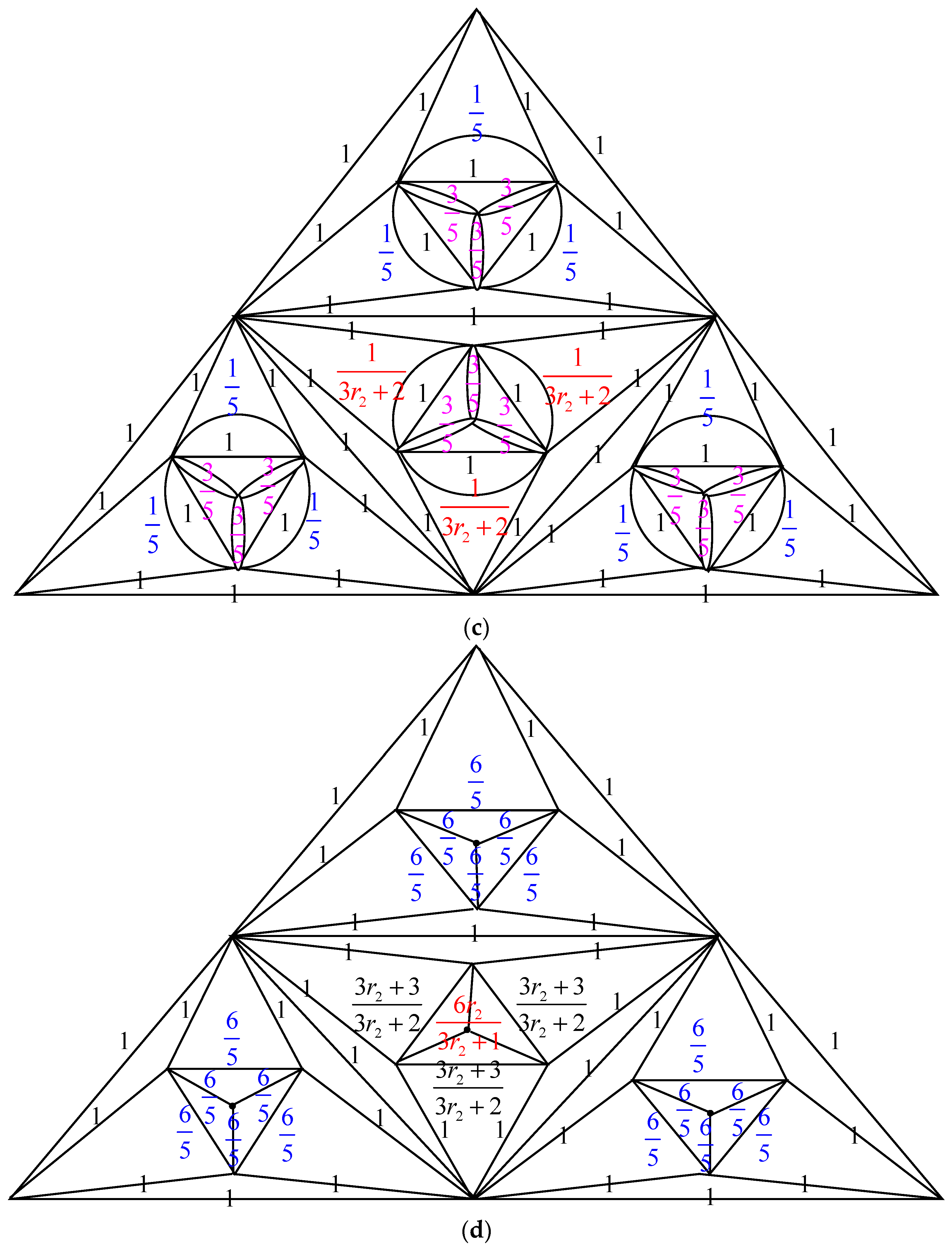
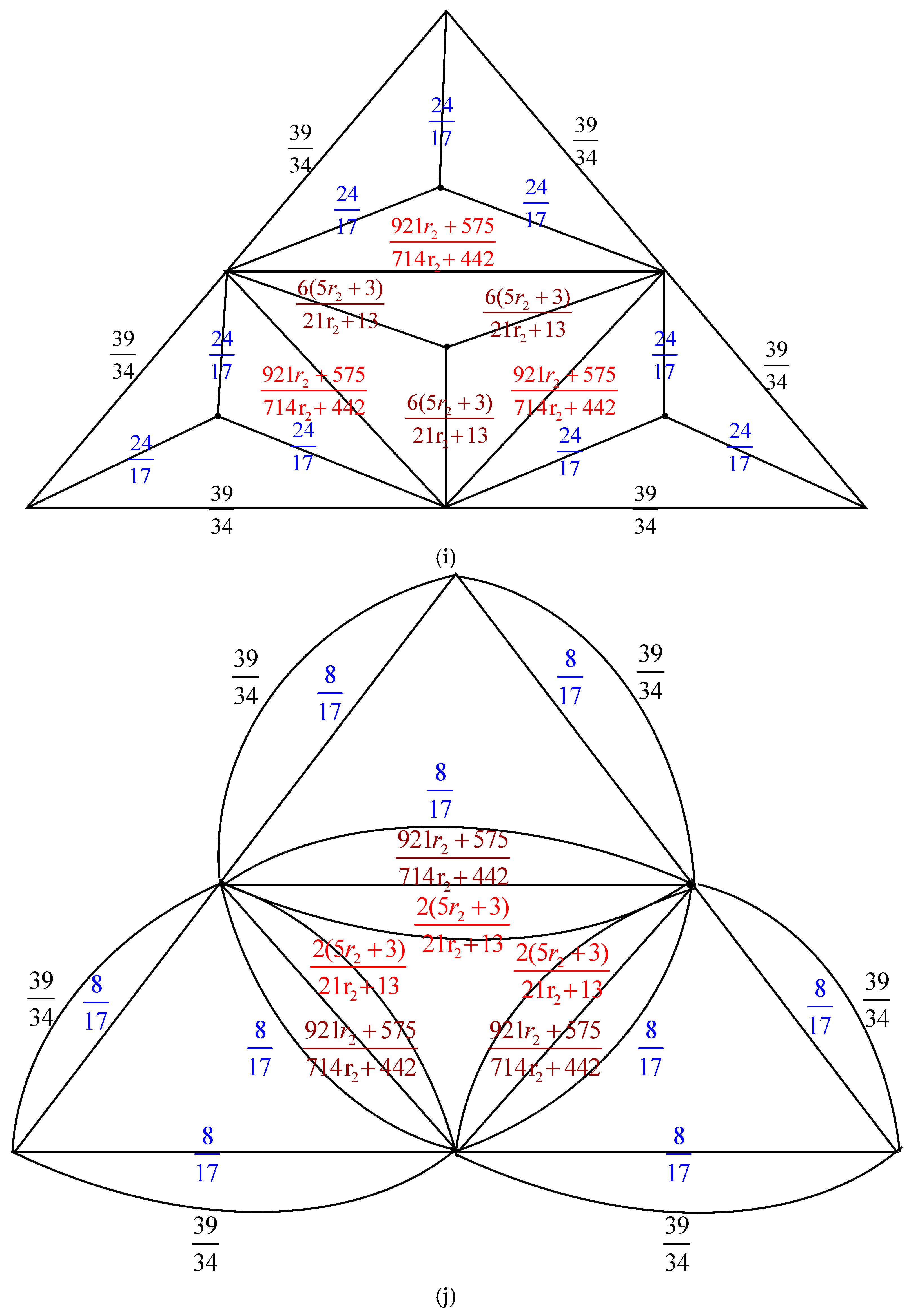
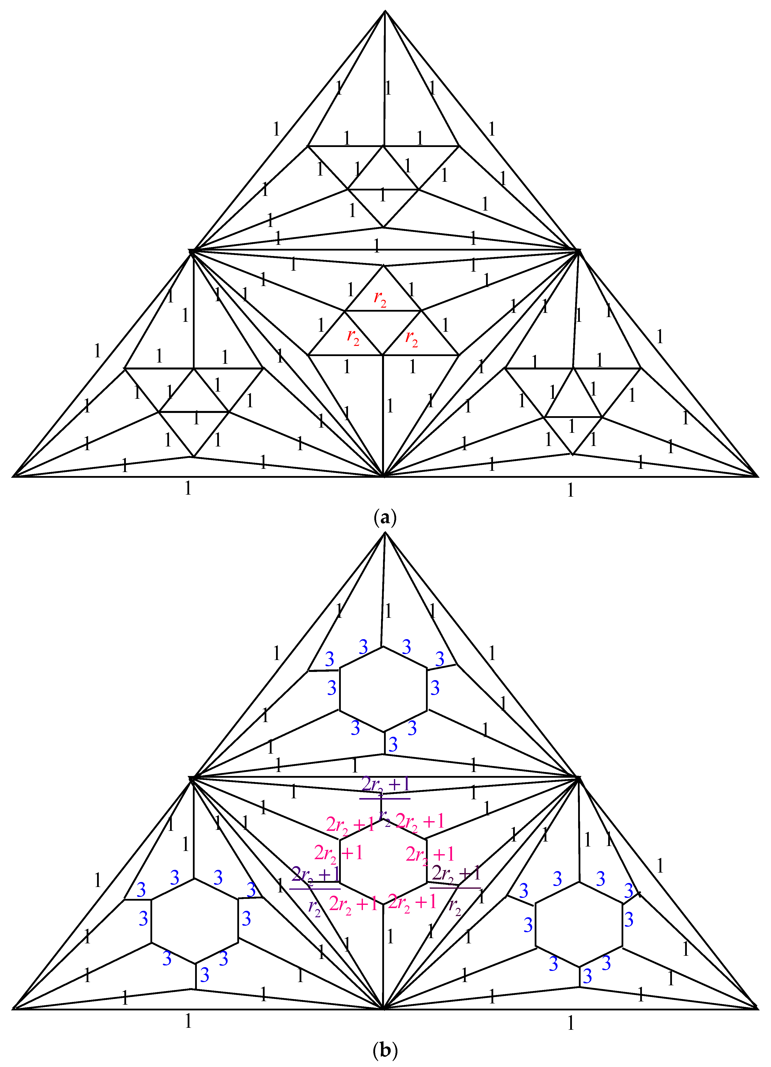
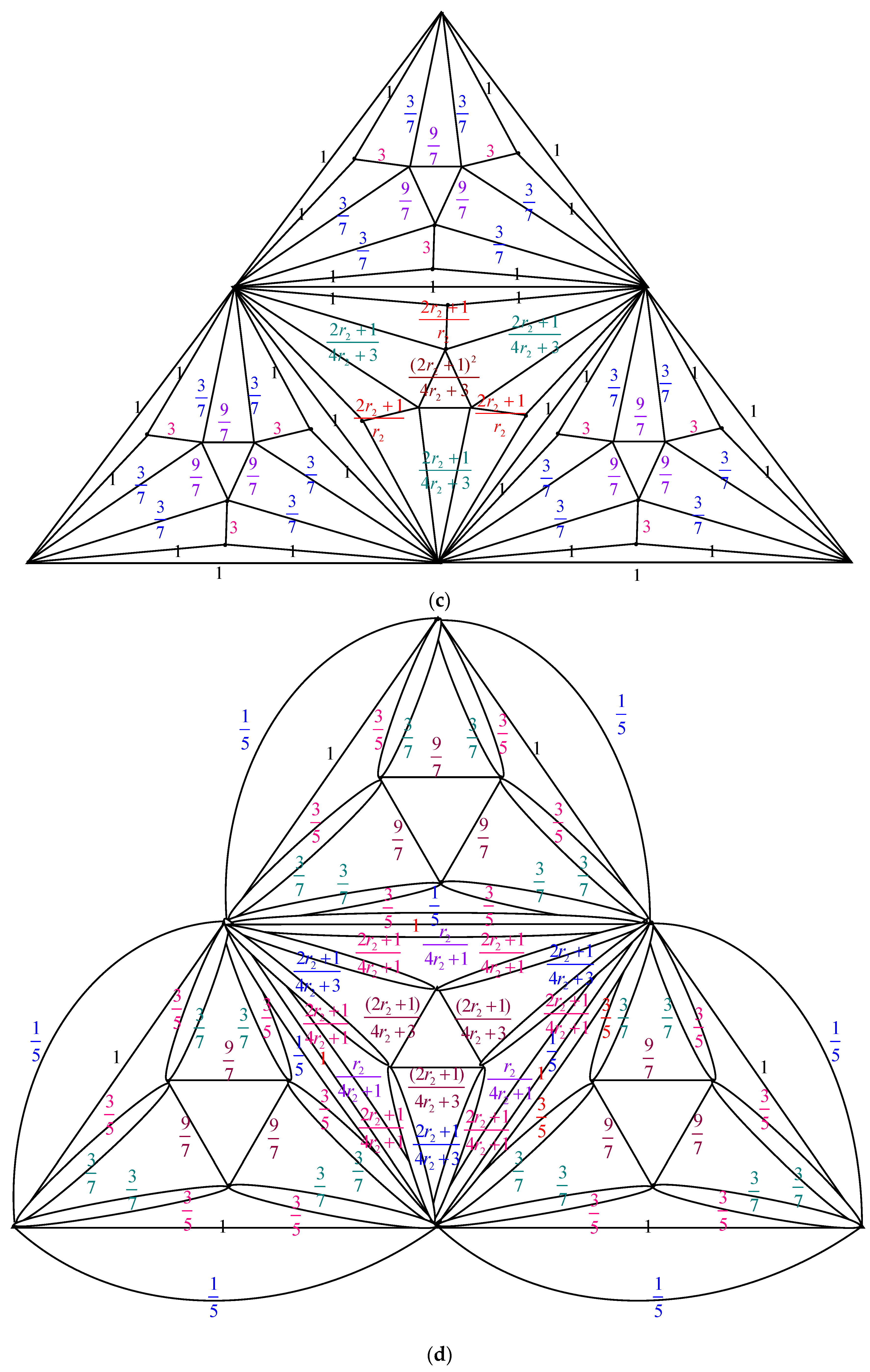
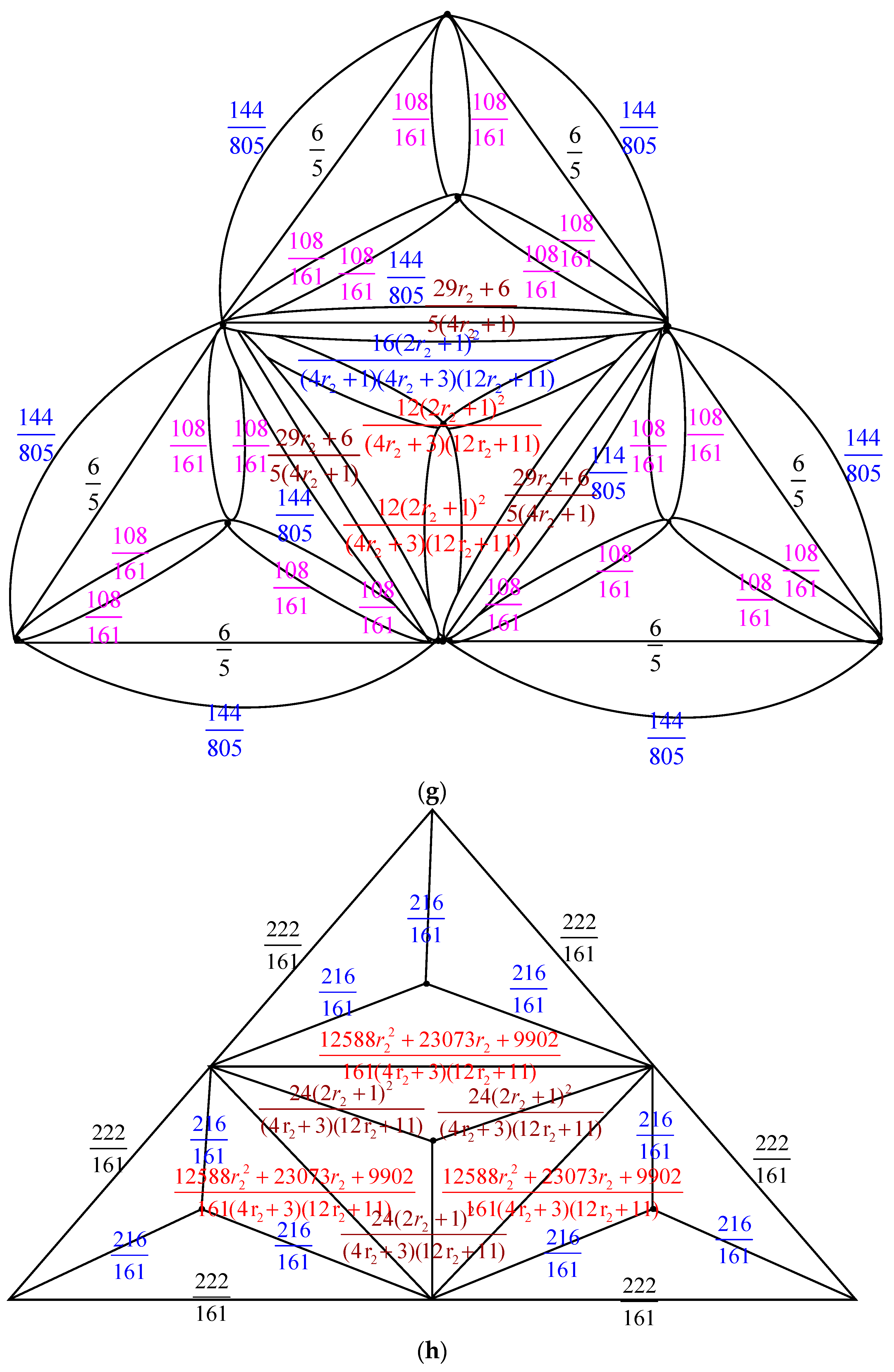
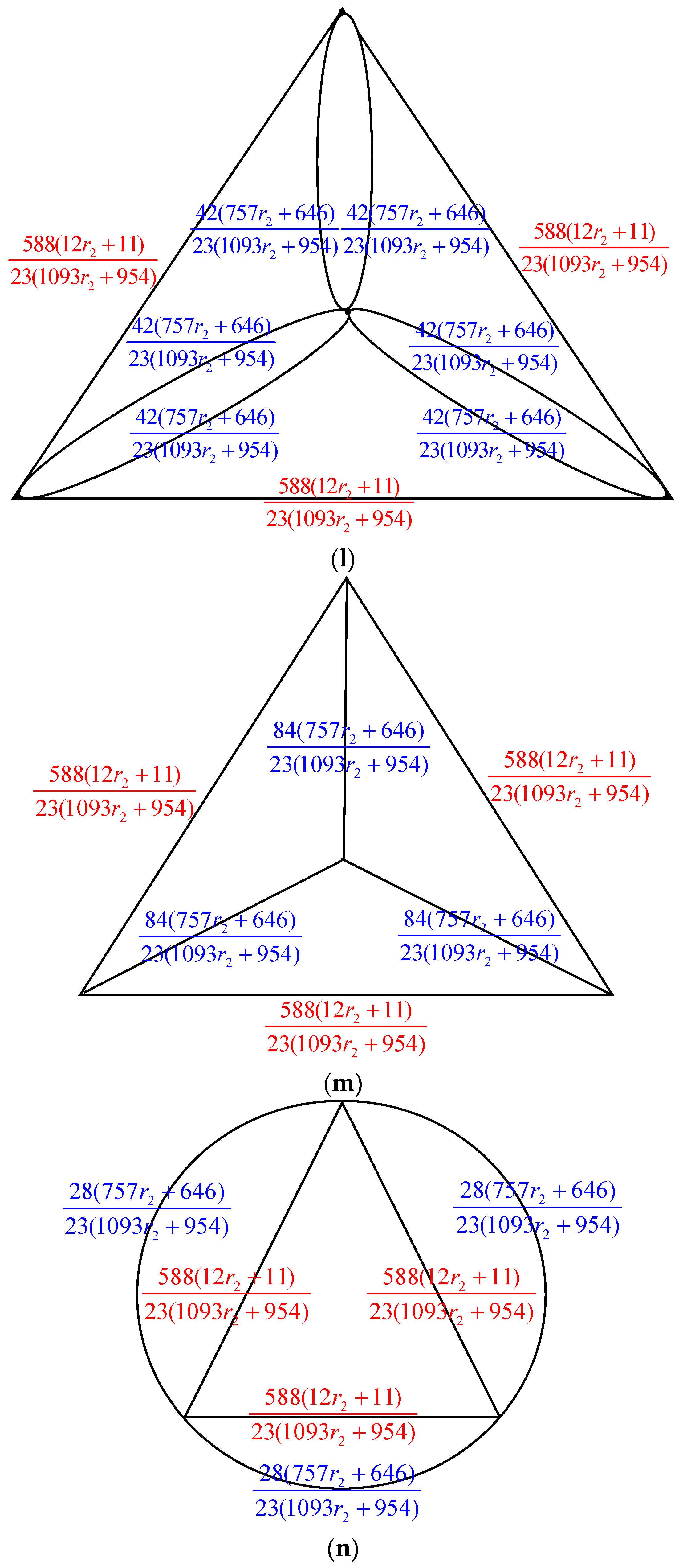
• Parallel edges: When two parallel edges in $G$, each with conductances $u$ and $v$, are merged into a single edge in $H$ with a conductance of $u+v$, the count of spanning trees, $\tau \left(H\right)$, remains unchanged compared to $\tau \left(G\right)$.
• Serial edges: If two serial edges in $G$, with conductances $a$ and $b$, are combined into a single edge in $H$ with a conductance of $ab/(a+b)$, then $\tau \left(H\right)$ can be calculated as $(1/(a+b)$ multiplied by $\tau \left(G\right)$.
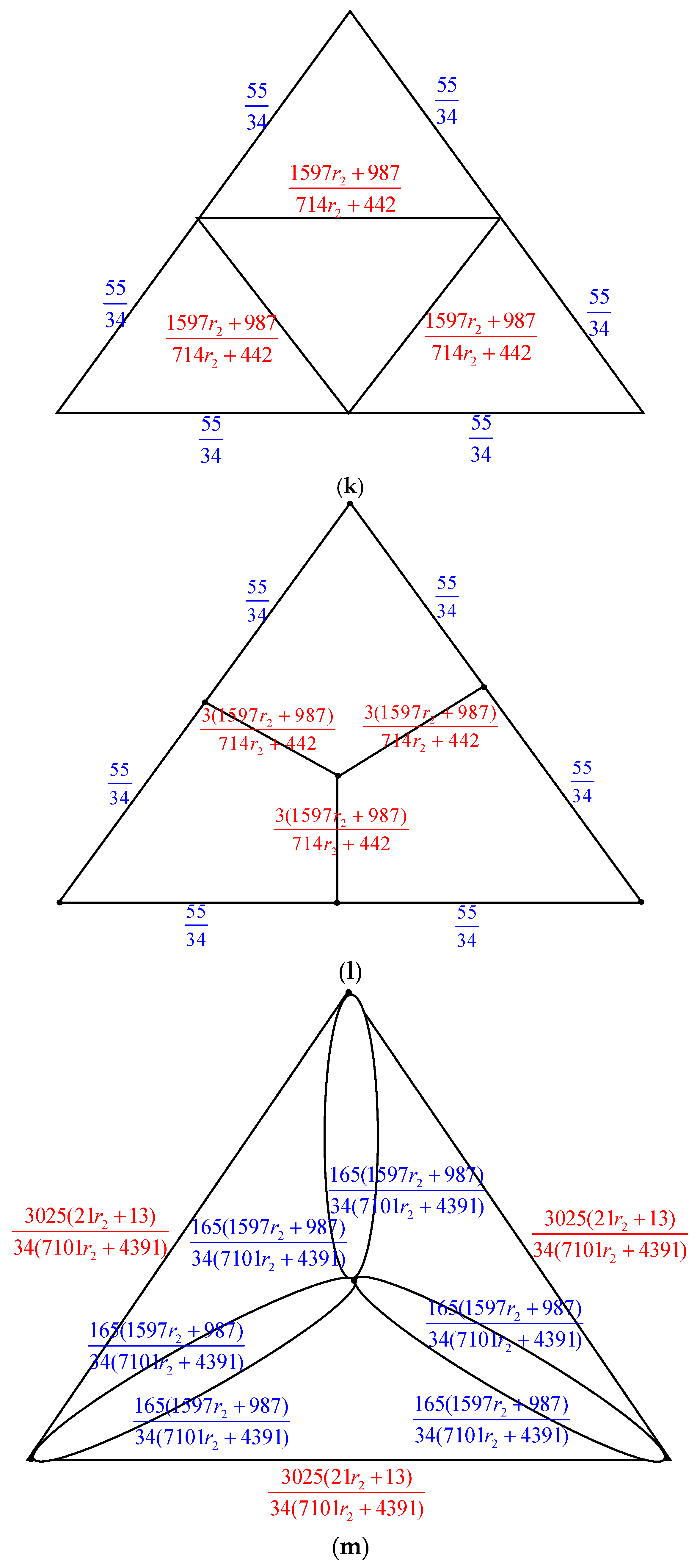
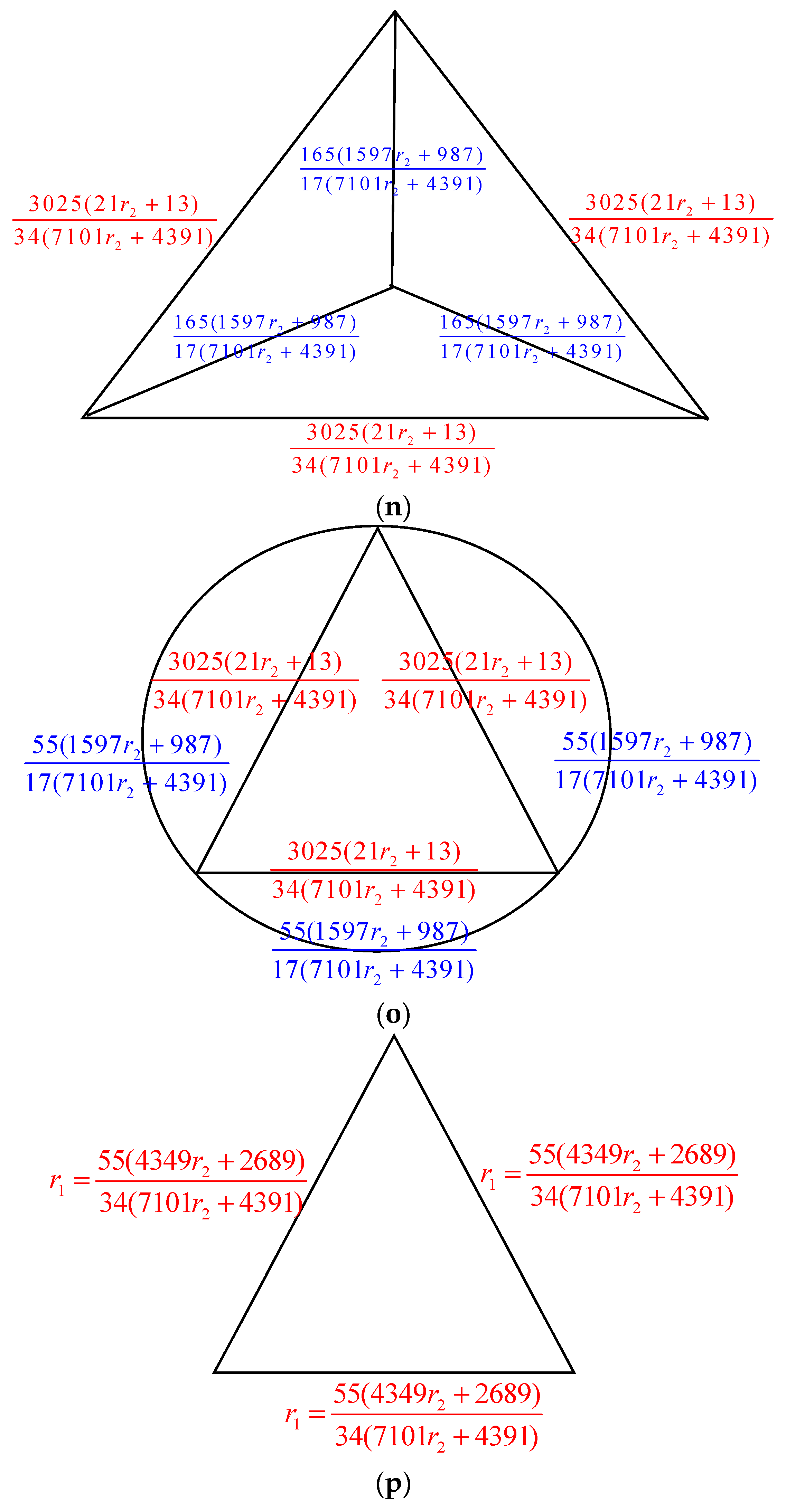
• Δ-Y Transformation: When a triangle in $G$, with conductances $a,b$, and $c$ is transformed into an electrically equivalent star graph in $H$ with conductances $u=\left(\mathit{ab}+\mathit{bc}+ca\right)/a,v=\left(\mathit{ab}+\mathit{bc}+ca\right)/b$, and $w=\left(\mathit{ab}+\mathit{bc}+ca\right)/c$, the count of spanning trees in $H$,$\tau \left(H\right)$, can be determined as ${\left(\mathit{ab}+\mathit{bc}+ca\right)}^2/abc$multiplied by $\tau \left(G\right)$.
• Y-Δ Transformation: If a star graph in $G$, with conductances $a,b$, and $c$, is converted into an electrically equivalent triangle in $H$ with conductances $u=bc/\left(a+b+c\right),v=ac/\left(a+b+c\right)$, and $w=ab/(a+b+c)$, then $\tau \left(H\right)$ is given by $1/(a+b+c)$ multiplied by $\tau \left(G\right)$.

2. Main Results

The goal in mathematics is always to derive a new structure from an existing one. This is also true in the realm of graphs, where a specified collection of graphs can be utilized to generate a significant number of new graphs. In this work, we will find the exact formula for the number of spanning trees of three new types of pyramidal graphs produced from the three nonahedral graphs with nine vertices denoted by $G_{1 }, G_{2 }$, and $G_{3 }$ shown in Figure 1.

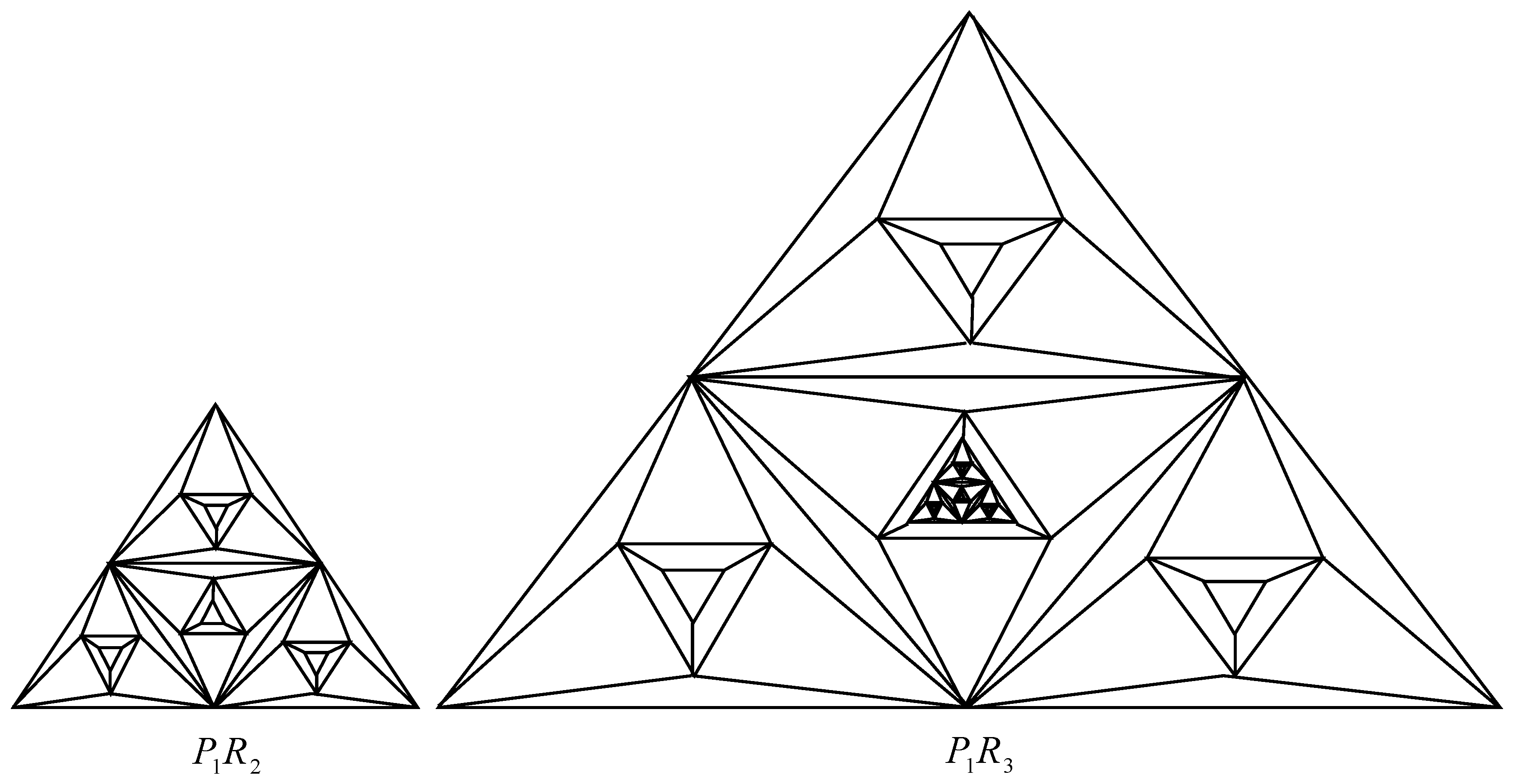
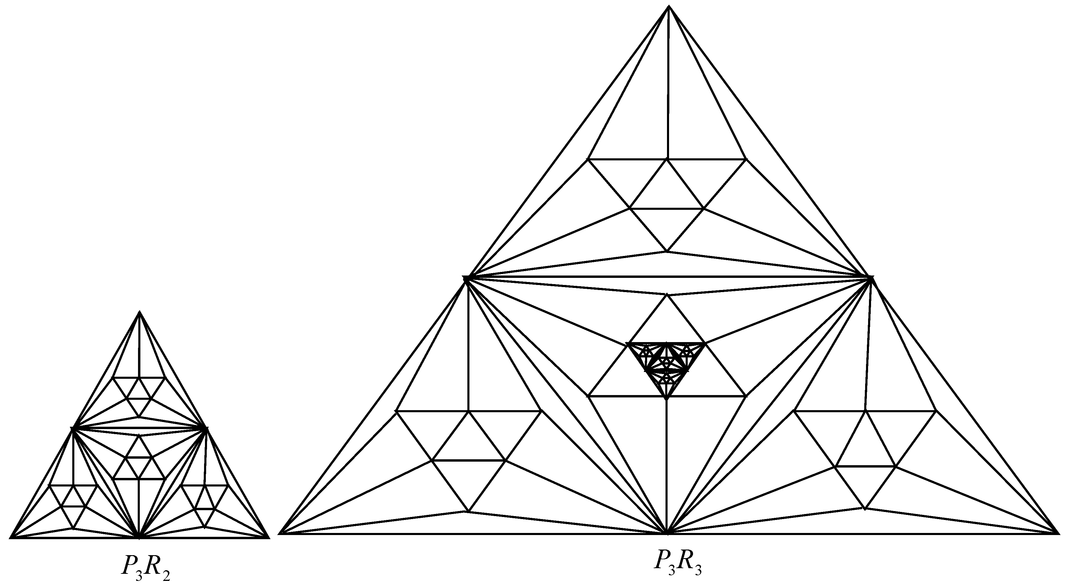
2.1. Number of Spanning Trees of Pyramid Graph $P_1{R}_n$ Based on Nonahedron Graph $G_1$

Using the graphs$P_1{R}_1$ (triangle or$K_3$) and $P_1{R}_2$, the pyramid graph $P_1{R}_n$ is defined recursively as follows: A copy of${ P}_1{R}_2$ is used to replace the middle triangle in$P_{1}R$ to create the graph $P_1{R}_3$. Generally speaking, $P_1{R}_{n }$is produced by substituting $P_1{R}_2$ for the middle triangle $P_1{R}_{n-1}$ (see Figure 2). The total vertices$\left|V\left(P_1{R}_n\right)\right|$ and edges $\left|E(P_1{R}_n)\right|$, according to this construction, are $\left|V\left(P_1{R}_n\right)\right|=27n-24$ and $\left|E(P_1{R}_n)\right|=60n-57$, $n=1,2,\dots$ The average degree of $P_1{R}_n$is in the large $n$limit, which is $4.44$.

Theorem 1.

The number of spanning trees in the pyramid graph$P_1{R}_n$ for  $n\ge 1$ is determined by

$$3\times {\left(27232\right)}^{n-1}{[ {\displaystyle \frac{{\left( \frac{7042221727+356052\sqrt{391194307}}{724201} \right)}^{n-1}\left( 394513805+19948\sqrt{391194307 }\right)-299\left(11102-\sqrt{391194307 }\right)}{{\left( \frac{7042221727+356052\sqrt{391194307} }{724201}\right)}^{n-1}\left( 400567658+20247\sqrt{391194307 }\right)-9373351}} ]}^2$$

$$\begin{gathered} {[\left( {\displaystyle \frac{46975785967481+2375080395\sqrt{391194307}}{782388614}}\right){\left( 59342+3\sqrt{391194307 } \right)}^{n-2} \\ +\left( {\displaystyle \frac{46975785967481-2375080395\sqrt{391194307}}{782388614}}\right){\left( 59342-3\sqrt{391194307} \right)}^{n-2}]}^2 \end{gathered}$$

Proof. 

${\mathrm{P}}_1{\mathrm{R}}_{\mathrm{j}}$ is changed to ${\mathrm{P}}_1{\mathrm{R}}_{\mathrm{j}-1}$ using the electrically equivalent transformation. The conversion procedure from ${\mathrm{P}}_1{\mathrm{R}}_2$ to ${\mathrm{P}}_1{\mathrm{R}}_1$ is shown in Figure 3.

Applying the Δ-Y transformation rule, we obtain $\mathsf{\tau }({\mathrm{H}}_1)=9^4{\mathrm{r}}_2\mathsf{\tau }({\mathrm{P}}_1{\mathrm{R}}_2).$

Using the rule of serial edges transformation, we obtain $\mathsf{\tau }({\mathrm{H}}_2)=({\displaystyle \frac{1}{4}}{)}^9({\displaystyle \frac{1}{3{\mathrm{r}}_2+1}}{)}^3\mathsf{\tau }({\mathrm{H}}_1)$.

Utilizing the Y-Δ transformation method, we obtain $\mathsf{\tau }({\mathrm{H}}_3)=({\displaystyle \frac{4}{9}}{)}^3({\displaystyle \frac{3{\mathrm{r}}_2+1}{9{\mathrm{r}}_2}})\mathsf{\tau }({\mathrm{H}}_2)$.

Using the transformation rule for parallel edges, we obtain $\mathsf{\tau }({\mathrm{H}}_4)=\mathsf{\tau }({\mathrm{H}}_3)$.

Utilizing the Δ-Y transformation method, we arrive at $\mathsf{\tau }({\mathrm{H}}_5)=9({\displaystyle \frac{45}{4}}{)}^3({\displaystyle \frac{4{\mathrm{r}}_2+1}{3{\mathrm{r}}_2+1}})\mathsf{\tau }({\mathrm{H}}_4).$

When we use the Δ-Y transformation rule again, we obtain $\mathsf{\tau }({\mathrm{H}}_6)=({\displaystyle \frac{4}{23}}{)}^9({\displaystyle \frac{3{\mathrm{r}}_2+1}{18{\mathrm{r}}_2+5}}{)}^3\mathsf{\tau }({\mathrm{H}}_5)$.

By using the transformation rule for parallel edges, we obtain $\mathsf{\tau }({\mathrm{H}}_7)=\mathsf{\tau }({\mathrm{H}}_6)$.

When the Y-Δ transformation rule is applied, we obtain $\mathsf{\tau }({\mathrm{H}}_8)=({\displaystyle \frac{23}{90}}{)}^3{\displaystyle \frac{18{\mathrm{r}}_2+5}{18(4{\mathrm{r}}_2+1)}}\mathsf{\tau }({\mathrm{H}}_7)$.

When the parallel edges transformation rule is used, we obtain $\mathsf{\tau }({\mathrm{H}}_9)=\mathsf{\tau }({\mathrm{H}}_8)$.

Using the Δ-Y transformation rule, we obtain $\mathsf{\tau }({\mathrm{H}}_{10})=9({\displaystyle \frac{919{\mathrm{r}}_2+254}{414{\mathrm{r}}_2+115}})\mathsf{\tau }({\mathrm{H}}_9)$.

When the Y-Δ transformation rule is applied, we obtain $\mathsf{\tau }({\mathrm{H}}_{11})=[{\displaystyle \frac{23(18{\mathrm{r}}_2+5)}{4089{\mathrm{r}}_2+1132}}{]}^3\mathsf{\tau }({\mathrm{H}}_{10})$.

Using the transformation rule for parallel edges, we obtain $\mathsf{\tau }({\mathrm{H}}_{12})=\mathsf{\tau }({\mathrm{H}}_{11})$.

Utilizing the Y-Δ transformation method, we arrive at $\mathsf{\tau }({\mathrm{H}}_{13})={\displaystyle \frac{23(4089{\mathrm{r}}_2+1132)}{666(919{\mathrm{r}}_2+254)}}\mathsf{\tau }({\mathrm{H}}_{12})$.

By using the transformation rule for parallel edges, we obtain ${\mathsf{\tau }(\mathrm{P}}_1{\mathrm{R}}_1)=\mathsf{\tau }({\mathrm{H}}_{14})$.

When these fourteen transformations are combined, we obtain

$$\begin{gathered} \tau \left(P_1{R}_2\right)=[{\displaystyle \frac{1}{9^4{r}_2}}\times 4^9\times {\left(3r_2+1\right)}^3\times {\left({\displaystyle \frac{9}{4}}\right)}^3\times \left({\displaystyle \frac{9r_2}{3r_2+1}}\right)\times {\left({\displaystyle \frac{4}{45}}\right)}^3\times {\displaystyle \frac{\left(3r_2+1\right)}{9\left(4r_2+1\right)}}\times {\left({\displaystyle \frac{23}{4}}\right)}^9\times {\left({\displaystyle \frac{18r_2+5}{3a+1}}\right)}^3 \\ \times {\left({\displaystyle \frac{90}{23}}\right)}^3\times {\displaystyle \frac{18\left(4r_2+1\right)}{18r_2+5}}\times {\displaystyle \frac{\left(414r_2+115\right)}{9\left(919r_2+254\right)}}\times {\left[{\displaystyle \frac{4089r_2+1132}{23\left(18r_2+5\right)}}\right]}^3\times {\displaystyle \frac{666\left(919r_2+254\right)}{23\left(4089r_2+1132\right)}} \\ \times {\left({\displaystyle \frac{92648r_2+25641}{94047r_2+26036}}\right)}^2]\tau \left(P_1{R}_1\right). \end{gathered}$$

Thus,

$$\tau \left(P_1{R}_2\right)=27232(94047r_2+26036{)}^2\tau (P_1{R}_1).$$

(3)

Further,

$$\begin{gathered} \tau (P_1{R}_n)=\prod _{i=2}^{n}27232(94047r_i+26036)\tau \left(P_1{R}_1\right) \\ =3\times (27232{)}^{n-1}{r}_1^2[ \prod _{i=2}^n(94047r_i+26036){]}^2 \end{gathered}$$

(4)

where ${\mathrm{r}}_{\mathrm{i}-1}={\displaystyle \frac{92648{\mathrm{r}}_{\mathrm{i}}+25641}{94047{\mathrm{r}}_{\mathrm{i}}+26036}}, \mathrm{i}=2,3,\dots ,\mathrm{n}.$

Its characteristic equation is $94047{\mathsf{\omega }}^2-66612\mathsf{\omega }-25641=0$ with roots ${\mathsf{\omega }}_1={\displaystyle \frac{11102-\sqrt{391194307}}{31349}}$ and ${\mathsf{\omega }}_1={\displaystyle \frac{11102+\sqrt{391194307}}{31349}}$.

Subtracting these two roots into both sides of ${\mathrm{r}}_{\mathrm{i}-1}={\displaystyle \frac{92648{\mathrm{r}}_{\mathrm{i}}+25641}{94047{\mathrm{r}}_{\mathrm{i}}+26036}}$, we obtain

$$\begin{gathered} r_{i-1}-{\displaystyle \frac{11102-\sqrt{391194307}}{31349}}={\displaystyle \frac{92648r_i+25641}{94047r_i+26036}}-{\displaystyle \frac{11102-\sqrt{391194307}}{31349}} \\ =(59342+3\sqrt{391194307}).{\displaystyle \frac{r_i-\frac{11102-\sqrt{391194307}}{31349}}{23(4089r_i+1132)}} \end{gathered}$$

(5)

$$\begin{gathered} r_{i-1}-{\displaystyle \frac{11102+\sqrt{391194307}}{31349}}={\displaystyle \frac{92648r_i+25641}{94047r_i+26036}}-{\displaystyle \frac{11102+\sqrt{391194307}}{31349}} \\ =(59342-3\sqrt{391194307}).{\displaystyle \frac{r_i-\frac{11102+\sqrt{391194307}}{31349}}{23(4089r_i+1132)}} \end{gathered}$$

(6)

Let ${\mathrm{x}}_{\mathrm{i}}={\displaystyle \frac{{\mathrm{r}}_{\mathrm{i}}-\frac{11102-\sqrt{391194307}}{31349}}{{\mathrm{r}}_{\mathrm{i}}-\frac{11102+\sqrt{391194307}}{31349}}}$. Then, by Equations (5) and (6), we obtain ${\mathrm{x}}_{\mathrm{i}-1}=({\displaystyle \frac{7042221727+356252\sqrt{391194307}}{724201}}){\mathrm{x}}_{\mathrm{i}}$ and ${\mathrm{x}}_{\mathrm{i}}=({\displaystyle \frac{7042221727+356252\sqrt{391194307}}{724201}}{)}^{\mathrm{n}-\mathrm{i}}{\mathrm{x}}_{\mathrm{n}}.$

Therefore, ${\mathrm{r}}_{\mathrm{i}}={\displaystyle \frac{(\frac{7042221727+356252\sqrt{391194307}}{724201}{)}^{\mathrm{n}-\mathrm{i}}(\frac{11102+\sqrt{391194307}}{31349}){\mathrm{x}}_{\mathrm{n}}-(\frac{11102-\sqrt{391194307}}{31349})}{(\frac{7042221727+356252\sqrt{391194307}}{724201}{)}^{\mathrm{n}-\mathrm{i}}{\mathrm{x}}_{\mathrm{n}}-1}}.$

Thus,

$$r_1={\displaystyle \frac{(\frac{7042221727+356252\sqrt{391194307}}{724201}{)}^{n-1}(\frac{11102+\sqrt{391194307}}{31349})x_n-(\frac{11102-\sqrt{391194307}}{31349})}{(\frac{7042221727+356252\sqrt{391194307}}{724201}{)}^{n-1}{x}_n-1}}.$$

(7)

Using the expression ${\mathrm{r}}_{\mathrm{n}-1}={\displaystyle \frac{92648{\mathrm{r}}_{\mathrm{n}}+25641}{94047{\mathrm{r}}_{\mathrm{n}}+26036}}$ and denoting the coefficients of $92648{\mathrm{r}}_{\mathrm{n}}+25641$ and $94047{\mathrm{r}}_{\mathrm{n}}+26036$ as ${\mathsf{\alpha }}_{\mathrm{n}}$ and ${\mathsf{\beta }}_{\mathrm{n}}$, we have

$$\begin{gathered} 94047r_n+26036={\delta }_0\left(92648r_n+25641\right)+{\sigma }_0\left(94047r_n+26036\right), \\ 94047r_{n-1}+26036={\displaystyle \frac{{\delta }_1\left(92648r_n+25641\right)+{\sigma }_1\left(94047r_n+26036\right)}{{\delta }_0\left(92648r_n+25641\right)+{\sigma }_0\left(94047r_n+26036\right)}}, \\ 94047r_{n-2}+26036={\displaystyle \frac{{\delta }_2(92648r_n+25641)+{\sigma }_2(94047r_n+26036)}{{\delta }_1(92648r_n+25641)+{\sigma }_1(94047r_n+26036)}}, \\ ⋮ \\ 94047r_{n-i}+26036={\displaystyle \frac{{\delta }_i(92648r_n+25641)+{\sigma }_i(94047r_n+26036)}{{\delta }_{i-1}(92648r_n+25641)+{\sigma }_{i-1}(94047r_n+26036)}}, \end{gathered}$$

(8)

$$94047r_{n-(i+1)}+26036={\displaystyle \frac{{\delta }_{i+1}(92648r_n+25641)+{\sigma }_{i+1}(94047r_n+26036)}{{\delta }_i(92648r_n+25641)+{\sigma }_i(794047r_n+26036)}},$$

(9)

$$94047r_2+26036={\displaystyle \frac{{\delta }_{n-2}(92648r_n+25641)+{\sigma }_{n-2}(94047r_n+26036)}{{\delta }_{n-3}(92648r_n+25641)+{\sigma }_{n-3}(94047r_n+26036)}},$$

Thus, we obtain

$$\tau (P_1{R}_n)=3\times (27232{)}^{n-1}{r}_1^2[{\delta }_{n-2}(92648r_n+25641)+{\sigma }_{n-2}(94047r_n+26036){]}^2$$

(10)

where ${\delta }_0=0, {\sigma }_0=1$ and ${\delta }_1=94047, {\sigma }_1=26036$. By the expression $r_{n-1}={\displaystyle \frac{92648r_n+25641}{94047r_n+26036}}$ and using Equations (8) and (9), we have

$${\delta }_{i+1}=118684{\delta }_i-724201{\delta }_{i-1}; {\sigma }_{i+1}=118684{\sigma }_i-724201{\sigma }_{i-1}$$

(11)

The characteristic equation of Equation (11) is ${\gamma }^2-118684\gamma +724201=0$ with roots ${\gamma }_1=59342+3\sqrt{391194307}$ and ${\gamma }_2=59342-3\sqrt{391194307}$.

The general solutions of Equation (11) are ${\delta }_i=a_1{\gamma }_1^i+a_2{\gamma }_2^i; {\sigma }_i=b_1{\gamma }_1^i+b_2{\gamma }_2^i$.

Using the initial conditions ${\delta }_0=0, {\sigma }_0=1$ and ${\delta }_1=94047, {\sigma }_1=26036$ yields

$$\begin{gathered} {\delta }_i={\displaystyle \frac{31349\sqrt{391194307}}{782388614}}(59342+3\sqrt{391194307}{)}^i-{\displaystyle \frac{31349\sqrt{391194307}}{782388614}}(59342-3\sqrt{391194307}{)}^i; \\ {\sigma }_i=\left({\displaystyle \frac{391194307-11102\sqrt{391194307}}{782388614}}\right(59342+3\sqrt{391194307}{)}^i+\left({\displaystyle \frac{391194307+11102\sqrt{391194307}}{782388614}}\right(59342-3\sqrt{391194307}{)}^i \end{gathered}$$

(12)

There is no electrically comparable transformation for $P_1{R}_n$ if $r_n=1$. When we enter Equation (12) into Equation (10), we obtain

$$\begin{gathered} \tau (P_1{R}_n)=3\times {\left(27232\right)}^{n-1}[\left({\displaystyle \frac{46975785967481+2375080395\sqrt{391194307}}{782388614}}\right){\left(59342+3\sqrt{391194307}\right)}^{n-2}+ \\ \left({\displaystyle \frac{46975785967481-2375080395\sqrt{391194307}}{782388614}}\right){\left(59342-3\sqrt{391194307}\right)}^{n-2}{]}^2, n\ge 2 \end{gathered}$$

(13)

Equation (13) is satisfied for $\mathrm{n}=1$. Consequently, the number of spanning trees in the pyramid graph ${\mathrm{P}}_1{\mathrm{R}}_{\mathrm{n}}$ is determined by

$$\begin{gathered} (P_1{R}_n)=3\times {\left(27232\right)}^{n-1}[\left({\displaystyle \frac{46975785967481+2375080395\sqrt{391194307}}{782388614}}\right){\left(59342+3\sqrt{391194307}\right)}^{n-2} \\ +\left({\displaystyle \frac{46975785967481-2375080395\sqrt{391194307}}{782388614}}\right){\left(59342-3\sqrt{391194307}\right)}^{n-2}{]}^2, n\ge 1 \end{gathered}$$

(14)

where

$$r_1={\displaystyle \frac{{\left(\frac{7042221727+356052\sqrt{391194307}}{724201}\right)}^{n-1}(394513805+19948\sqrt{391194307})-299(11102-\sqrt{391194307})}{{\left(\frac{7042221727+356052\sqrt{391194307}}{724201}\right)}^{n-1}\left(400567658+20247\sqrt{391194307}\right)-9373351, n\ge 1}}$$

(15)

Equation (15) can be inserted into Equation (14), yielding the desired result. □

2.2. Number of Spanning Trees of Pyramid Graph $P_2{R}_n$ Based on the Nonahedron $G_2$

Using the graphs $P_2{R}_1$ (triangle or$K_3$) and $P_2{R}_2$, the pyramid graph $P_2{R}_n$ is defined recursively as follows: A copy of ${ P}_2{R}_2$ is used to replace the middle triangle in$P_2{R}_2$ to create the graph $P_2{R}_3$. Generally speaking, $P_2{R}_n$ is produced by substituting $P_2{R}_2$ for the middle triangle $P_2{R}_{n-1}$ (see Figure 4). The total vertices $\left|V\left(P_2{R}_n\right)\right|$ and edges $\left|E(P_2{R}_n)\right|$, according to this construction, are $\left|V\left(P_2{R}_n\right)\right|=27n-24$ and $\left|E(P_2{R}_n)\right|=69n-66$, $n=1,2,\dots$

The average degree of $P_2{R}_n$ is in the large $n$limit, which is $5.11$.

Theorem 2.

The number of spanning trees in the pyramid graph${ P}_2{R}_n$ for  $n\ge 1$ is determined by

$$\begin{gathered} 3\times {\left( \mathrm{957,440} \right)}^{n-1}{\left({\displaystyle \frac{{\left(\frac{ 150916709321+1165467\sqrt{16767746169} }{6993800}\right)}^{n-1}\left( 50412258453+389329\sqrt{16767746169}\right)-3638\left(29967-\sqrt{16767746169 } \right)}{9{\left(\frac{ 150916709321+1165467\sqrt{16767746169}}{6993800} \right)}^{n-1}\left( 5654310715+43663\sqrt{16767746169 }\right)-585557928}}\right)}^2 \\ \begin{array}{c}\times [ \left( 195364+8432585344\sqrt{{\displaystyle \frac{3}{5589248723 }}}\right){\left( {\displaystyle \frac{388489+3\sqrt{16767746169}}{2}} \right)}^{n-2}\\ +\left(195364-8432585344\sqrt{{\displaystyle \frac{3}{5589248723}}} \right){ \left( {\displaystyle \frac{388489-3\sqrt{16767746169} }{2}}\right)}^{n-2}{]}^2\end{array} \end{gathered}$$

Proof. 

${\mathrm{P}}_2{\mathrm{R}}_{\mathrm{j}}$ is changed to ${\mathrm{P}}_2{\mathrm{R}}_{\mathrm{j}-1}$ using the electrically equivalent transformation. The conversion procedure from ${\mathrm{P}}_2{\mathrm{R}}_2$ to ${\mathrm{P}}_2{\mathrm{R}}_1$ is shown in Figure 5.

Utilizing the Δ-Y transformation method, we obtain $\mathsf{\tau }({\mathrm{H}}_1)=9^4{\mathrm{r}}_2\mathsf{\tau }({\mathrm{P}}_2{\mathrm{R}}_2)$.

Using the Y-Δ transformation rule, we have $\mathsf{\tau }({\mathrm{H}}_2)=({\displaystyle \frac{1}{5}}{)}^9({\displaystyle \frac{1}{3{\mathrm{r}}_2+2}}{)}^3\mathsf{\tau }({\mathrm{H}}_1)$.

Using the rule of parallel edges transformation, we obtain $\mathsf{\tau }({\mathrm{H}}_3)=\mathsf{\tau }({\mathrm{H}}_2)$.

When we use the Y-Δ transformation rule, we obtain $\mathsf{\tau }({\mathrm{H}}_4)=({\displaystyle \frac{5}{18}}{)}^3({\displaystyle \frac{3{\mathrm{r}}_2+2}{18{\mathrm{r}}_2}})\mathsf{\tau }({\mathrm{H}}_3)$.

Using the rule of parallel edges transformation, we obtain $\mathsf{\tau }({\mathrm{H}}_5)=\mathsf{\tau }({\mathrm{H}}_4)$.

When the Δ-Y transformation rule is applied, we obtain $\mathsf{\tau }({\mathrm{H}}_6)=9^4({\displaystyle \frac{8}{5}}{)}^3({\displaystyle \frac{5{\mathrm{r}}_2+3}{3{\mathrm{r}}_2+2}}{)}^3\mathsf{\tau }({\mathrm{H}}_5)$.

Using the Y-Δ transformation rule, we have $\mathsf{\tau }({\mathrm{H}}_7)=({\displaystyle \frac{5}{34}}{)}^9({\displaystyle \frac{3{\mathrm{r}}_2+2}{21{\mathrm{r}}_2+13}}{)}^3\mathsf{\tau }({\mathrm{H}}_6)$.

Applying the parallel edges transformation rule, we obtain $\mathsf{\tau }({\mathrm{H}}_8)=\mathsf{\tau }({\mathrm{H}}_7)$.

Utilizing the Y-Δ transformation method, we arrive at $\mathsf{\tau }({\mathrm{H}}_9)=({\displaystyle \frac{17}{72}}{)}^3{\displaystyle \frac{21{\mathrm{r}}_2+13}{18(5{\mathrm{r}}_2+3)}}\mathsf{\tau }({\mathrm{H}}_8)$.

Using the transformation rule for parallel edges, we have $\mathsf{\tau }({\mathrm{H}}_{10})=\mathsf{\tau }({\mathrm{H}}_9)$.

Using the Δ-Y transformation rule, we obtain $\mathsf{\tau }({\mathrm{H}}_{11})=9({\displaystyle \frac{1579{\mathrm{r}}_2+987}{714{\mathrm{r}}_2+442}})\mathsf{\tau }({\mathrm{H}}_{10})$.

Utilizing the Y-Δ transformation method, we obtain $\mathsf{\tau }({\mathrm{H}}_{12})=({\displaystyle \frac{714{\mathrm{r}}_2+442}{7101{\mathrm{r}}_2+4391}}{)}^3\mathsf{\tau }({\mathrm{H}}_{11})$.

By using the transformation rule for parallel edges, we obtain $\mathsf{\tau }({\mathrm{H}}_{13})=\mathsf{\tau }({\mathrm{H}}_{12})$.

Applying the Y-Δ transformation rule, we obtain $\mathsf{\tau }({\mathrm{H}}_{14})={\displaystyle \frac{17(7101{\mathrm{r}}_2+4391)}{495(1597{\mathrm{r}}_2+987)}}\mathsf{\tau }({\mathrm{H}}_{13})$.

Using the rule of parallel edges transformation, we have $\mathsf{\tau }({\mathrm{P}}_2{\mathrm{R}}_2)=\mathsf{\tau }({\mathrm{H}}_{14})$.

When these fifteen transformations are combined, we obtain

$$\begin{gathered} \tau (P_2{R}_2)=[{\displaystyle \frac{1}{9^{4}a}}\times 5^9\times {(3a+2)}^3\times {({\displaystyle \frac{18}{5}})}^3\times ({\displaystyle \frac{18a}{3a+2}})\times {\displaystyle \frac{1}{9^4}}{({\displaystyle \frac{5}{8}})}^3\times {\displaystyle \frac{(3a+2)}{(5a+3)}}\times {({\displaystyle \frac{34}{5}})}^9\times {({\displaystyle \frac{21a+13}{3a+2}})}^3\times {({\displaystyle \frac{72}{17}})}^3 \\ \times ({\displaystyle \frac{18(5a+3)}{21a+13}})\times {\displaystyle \frac{(714a+442)}{9(1597a+987)}}\times {({\displaystyle \frac{7101a+4391}{714a+442}})}^3\times {\displaystyle \frac{495(1597a+987)}{17(7101a+4391)}} \\ \times {({\displaystyle \frac{55(4349a+2689)}{34(7101a+4391)}})}^2\tau (P_2{R}_1) \end{gathered}$$

Thus,

$$\tau (P_2{R}_n)=957440(241434r_2+149294{)}^2\tau (P_2{R}_1)$$

(16)

Further,

$$\tau (P_2{R}_n)=\prod _{i=2}^{n}957440(241434r_i+149294{)}^2\tau (P_2{R}_1)$$

$$=3\times (957440{)}^{n-1}{r}_1^2[\prod _{i=2}^n(241434r_i+149294){]}^2$$

(17)

where ${\mathrm{r}}_{\mathrm{i}-1}={\displaystyle \frac{239195{\mathrm{r}}_{\mathrm{i}}+147985}{241434{\mathrm{r}}_{\mathrm{i}}+149294}}, \mathrm{i}=2,3,\dots ,\mathrm{n}.$ Its characteristic equation is $241434{\mathsf{\omega }}^2-89901\mathsf{\omega }-147895=0$, with roots ${\mathsf{\omega }}_1={\displaystyle \frac{29967-\sqrt{16767746169}}{160956}}$ and ${\mathsf{\omega }}_2={\displaystyle \frac{29967+\sqrt{16767746169}}{160956}}$. Subtracting these two roots into both sides of ${\mathrm{r}}_{\mathrm{i}-1}={\displaystyle \frac{239195{\mathrm{r}}_{\mathrm{i}}+147895}{241434{\mathrm{r}}_{\mathrm{i}}+149294}}$, we obtain

$${\begin{array}{c} \\ r\end{array}}_{i-1}-{\displaystyle \frac{29967-\sqrt{16767746169}}{160956}}={\displaystyle \frac{239195r_i+147985}{241434r_i+149294}}-{\displaystyle \frac{29967-\sqrt{16767746169}}{160956}}$$

$$=(388489+3\sqrt{16767746169}).{\displaystyle \frac{r_i-\frac{29967-\sqrt{16767746169}}{160956}}{68(7101r_i+4391)}}$$

(18)

$$r_{i-1}-{\displaystyle \frac{29967+\sqrt{16767746169}}{160956}}={\displaystyle \frac{239195r_i+147985}{241434r_i+149294}}-{\displaystyle \frac{29967+\sqrt{16767746169}}{160956}}$$

$$=(388489-3\sqrt{16767746169}).{\displaystyle \frac{r_i-\frac{29967+\sqrt{16767746169}}{160956}}{68(7101r_i+4391)}}$$

(19)

Let ${\mathrm{x}}_{\mathrm{i}}={\displaystyle \frac{{\mathrm{r}}_{\mathrm{i}}-\frac{29967-\sqrt{16767746169}}{160956}}{{\mathrm{r}}_{\mathrm{i}}-\frac{29967+\sqrt{16767746169}}{160956}}}$. Then, by Equations (18) and (19), we obtain ${\mathrm{x}}_{\mathrm{i}-1}=({\displaystyle \frac{150916709321+1165467\sqrt{16767746169}}{6993800}}){\mathrm{x}}_{\mathrm{i}}$ and ${\mathrm{x}}_{\mathrm{i}-1}=({\displaystyle \frac{150916709321+1165467\sqrt{16767746169}}{6993800}}{)}^{\mathrm{n}-\mathrm{i}}{\mathrm{x}}_{\mathrm{i}}$

Therefore, ${\mathrm{r}}_{\mathrm{i}}={\displaystyle \frac{(\frac{150916709321+1165467\sqrt{16767746169}}{6993800}{)}^{\mathrm{n}-\mathrm{i}}(\frac{29967+\sqrt{16767746169}}{160956}){\mathrm{x}}_{\mathrm{n}}-\frac{29967-\sqrt{16767746169}}{160956}}{(\frac{150916709321+1165467\sqrt{16767746169}}{6993800}{)}^{\mathrm{n}-\mathrm{i}}{\mathrm{x}}_{\mathrm{n}}-1}}.$

Thus,

$$r_1={\displaystyle \frac{( \frac{150916709321+1165467\sqrt{16767746169}}{6993800}{ )}^{n-1}( \frac{29967+\sqrt{16767746169}}{160956} )x_n-\frac{29967-\sqrt{16767746169}}{160956}}{( \frac{150916709321+1165467\sqrt{16767746169}}{6993800}{ )}^{n-1}{x}_n-1}}.$$

(20)

Using the expression $r_{n-1}={\displaystyle \frac{239195r_n+147895}{241434r_n+149294}}$ and denoting the coefficients of $239195r_n+147895$ and $241434r_n+149294$ as ${\alpha }_n$ and ${\beta }_n$, we have

$$\begin{gathered} 241434r_n+149294={\delta }_0\left(239195r_n+147895\right)+{\sigma }_0\left(241434r_n+149294\right), \\ 241434r_{n-1}+149294={\displaystyle \frac{{\delta }_1\left(239195r_n+147895\right)+{\sigma }_1\left(241434r_n+149294\right)}{{\delta }_0\left(239195r_n+147895\right)+{\sigma }_0\left(241434r_n+149294\right)}}, \\ 241434r_{n-2}+149294={\displaystyle \frac{{\delta }_2\left(239195r_n+147895\right)+{\sigma }_2\left(241434r_n+149294\right)}{{\delta }_1\left(239195r_n+147895\right)+{\sigma }_1\left(241434r_n+149294\right)}} \\ ⋮ \end{gathered}$$

$$241434r_{n-i}+149294={\displaystyle \frac{{\delta }_i(239195r_n+147895)+{\sigma }_i(241434r_n+149294)}{{\delta }_{i-1}(239195r_n+147895)+{\sigma }_{i-1}(241434r_n+149294)}},$$

(21)

$$\begin{gathered} 241434r_{n-(i+1)}+149294={\displaystyle \frac{{\delta }_{i+1}(239195r_n+147895)+{\sigma }_{i+1}(241434r_n+149294)}{{\delta }_i(239195r_n+147895)+{\sigma }_i(241434r_n+149294)}}, \\ ⋮ \end{gathered}$$

(22)

$$241434r_2+149294={\displaystyle \frac{{\delta }_{n-2}(239195r_n+147895)+{\sigma }_{n-2}(241434r_n+149294)}{{\delta }_{n-3}(239195r_n+147895)+{\sigma }_{n-3}(241434r_n+149294)}},$$

Thus, we obtain

$$\tau (P_2{R}_2)=3\times (957440{)}^{n-1}{r}_1^2[{\delta }_{n-2}(239195r_n+147895)+{\sigma }_{n-2}(241434r_n+149294){]}^2$$

(23)

where ${\mathsf{\delta }}_0=0, {\mathsf{\sigma }}_0=1$ and ${\mathsf{\delta }}_1=241434, {\mathsf{\sigma }}_1=149294$. By the expression ${\mathrm{r}}_{\mathrm{n}-1}={\displaystyle \frac{239195{\mathrm{r}}_{\mathrm{n}}+147895}{241434{\mathrm{r}}_{\mathrm{n}}+149294}}$ and using Equations (21) and (22), we have

$${\delta }_{i+1}=388489{\delta }_i-3496900{\delta }_{i-1}; {\sigma }_{i+1}=388489{\sigma }_i-3496900{\sigma }_{i-1}$$

(24)

The characteristic equation of Equation (24) is ${\mathsf{\gamma }}^2-388489\mathsf{\gamma }+3496900=0$ with roots ${\mathsf{\gamma }}_1={\displaystyle \frac{388489+3\sqrt{16767746169}}{2}}$ and ${\mathsf{\gamma }}_2={\displaystyle \frac{388489-3\sqrt{16767746169}}{2}}$. The general solutions of Equation (24) are ${\mathsf{\delta }}_{\mathrm{i}}={\mathrm{a}}_1{\mathsf{\gamma }}_1^{\mathrm{i}}+{\mathrm{a}}_2{\mathsf{\gamma }}_2^{\mathrm{i}};{\mathsf{\sigma }}_{\mathrm{i}}={\mathrm{b}}_1{\mathsf{\gamma }}_1^{\mathrm{i}}+{\mathrm{b}}_2{\mathsf{\gamma }}_2^{\mathrm{i}}$.

Using the initial conditions ${\mathsf{\delta }}_0=0, {\mathsf{\sigma }}_0=1$ and ${\mathsf{\delta }}_1=241434, {\mathsf{\sigma }}_1=149294$ yields

$${\delta }_i={\displaystyle \frac{26826\sqrt{16767746169}}{5589248723}}({\displaystyle \frac{388489+3\sqrt{16767746169}}{2}}{)}^i-{\displaystyle \frac{26826\sqrt{16767746169}}{5589248723}}({\displaystyle \frac{388489-3\sqrt{16767746169}}{2}}{)}^i;$$

$$\begin{gathered} {\sigma }_i=({\displaystyle \frac{5589248723-9989\sqrt{16767746169}}{11178497446}}({\displaystyle \frac{388489+3\sqrt{16767746169}}{2}}{)}^i \\ +({\displaystyle \frac{5589248723+9989\sqrt{16767746169}}{11178497446}})({\displaystyle \frac{388489-3\sqrt{16767746169}}{2}}{)}^i \end{gathered}$$

(25)

There is no electrically equivalent transformation in ${\mathrm{P}}_2{\mathrm{R}}_{\mathrm{n}}$ if ${\mathrm{r}}_{\mathrm{n}}=1$. When we insert Equation (25) into Equation (23), we obtain

$$\begin{gathered} \tau \left(P_2{R}_n\right)=3\times {\left(957440\right)}^{n-1}[\left( 195364+8432585344\sqrt{{\displaystyle \frac{3}{5589248723}}} \right){\left( {\displaystyle \frac{388489+3\sqrt{16767746169}}{2}} \right)}^{n-2} \\ +\left(195364-8432585344\sqrt{{\displaystyle \frac{3}{5589248723 }}}\right){\left( {\displaystyle \frac{388489-3\sqrt{16767746169}}{2}} \right)}^{n-2}{]}^2, n\ge 2. \end{gathered}$$

(26)

Equation (26) is satisfied when $\mathrm{n}=1$ and $\mathsf{\tau }\left({\mathrm{P}}_2{\mathrm{R}}_1\right)=3$. Consequently, the number of spanning trees of the pyramid graph ${\mathrm{P}}_2{\mathrm{R}}_{\mathrm{n}}$ is determined by

$$\begin{gathered} \tau \left(P_2{R}_n\right)=3\times {\left(957440\right)}^{n-1}[ \left(195364+8432585344\sqrt{{\displaystyle \frac{3}{5589248723}}}\right){\left({\displaystyle \frac{388489+3\sqrt{16767746169}}{2}} \right)}^{n-2} \\ +\left(195364-8432585344\sqrt{{\displaystyle \frac{3}{5589248723}}}\right){\left({\displaystyle \frac{ 388489-3\sqrt{16767746169}}{2}} \right)}^{n-2}{]}^2, n\ge 1. \end{gathered}$$

(27)

where

$$r_1={\displaystyle \frac{{\left( \frac{150916709321+1165467\sqrt{16767746169}}{6993800} \right)}^{n-1}\left( 50412258453+389329\sqrt{16767746169} \right)-3638\left( 29967-\sqrt{16767746169 }\right)}{9{\left( \frac{150916709321+1165467\sqrt{16767746169}}{6993800} \right)}^{n-1}\left( 5654310715+43663\sqrt{16767746169} \right)-585557928}}, n\ge 1.$$

(28)

The required result is obtained by inserting Equation (28) into Equation (27). □

2.3. Number of Spanning Trees of Pyramid Graph $P_3{R}_n$ Based on the Nonahedron Graph $G_3$

Using the graphs$P_3{R}_1$ (triangle or$K_3$) and $P_3{R}_2$, the pyramid graph $P_3{R}_n$ is defined recursively as follows: A copy of${ P}_3{R}_2$ is used to replace the middle triangle in$P_3{R}_2$ to create the graph $P_3{R}_3$. Generally speaking, $P_3{R}_n$ is produced by substituting $P_3{R}_2$ for the middle triangle $P_3{R}_{n-1}$ (refer to Figure 6). The total vertices$\left|V\left(P_3{R}_n\right)\right|$ and edges $\left|E(P_3{R}_n)\right|$, according to this construction, are $\left|V\left(P_3{R}_n\right)\right|=27n-24$ and $\left|E(P_3{R}_n)\right|=78n-75$, $n=1,2,\dots$

The average degree of $P_3{R}_n$is in the large $n$limit, which is $5.78$.

Theorem 3.

The number of spanning trees in the pyramid graph${ P}_3{R}_n$ for$n\ge 1$ is determined by

$$\begin{gathered} 3\times {\left(71221248\right)}^{n-1}{\left[{\displaystyle \frac{{\left( \frac{628563359+25097\sqrt{627267309}}{1296050} \right)}^{n-1}\left(412155311+16565\sqrt{627267309 }\right)+1909\left( 3155-\sqrt{627267309 } \right)}{{\left( \frac{628563359+25097\sqrt{627267309}}{1296050} \right)}^{n-1}\left( 370187855+14656\sqrt{627267309} \right)+47990351}}\right]}^2 \\ \begin{array}{c}[( {\displaystyle \frac{47081}{2}}+{\displaystyle \frac{392999919\sqrt{\frac{3}{209089103}}}{2}} ){\left(25097+\sqrt{627267309} \right)}^{n-2}+\\ ( {\displaystyle \frac{47081}{2}}-{\displaystyle \frac{392999919\sqrt{\frac{3}{209089103}}}{2}} ){( 25097-\sqrt{627267309} )}^{n-2}{]}^2\end{array} \end{gathered}$$

Proof. 

${\mathrm{P}}_3{\mathrm{R}}_{\mathrm{j}}$ is changed to ${\mathrm{P}}_3{\mathrm{R}}_{\mathrm{j}-1}$ using the electrically equivalent transformation. The conversion procedure from ${\mathrm{P}}_3{\mathrm{R}}_2$ to ${\mathrm{P}}_3{\mathrm{R}}_1$ is shown in Figure 7.

Utilizing the Δ-Y transformation method, we obtain $\tau (H_1)=9^9({\displaystyle \frac{(2r_2+1{)}^2}{r_2}}{)}^3\tau (P_3{R}_2)$.

When the Y-Δ transformation rule is applied, we obtain $\tau (H_2)=({\displaystyle \frac{1}{7}}{)}^9({\displaystyle \frac{1}{4r_2+3}}{)}^3\tau (H_1)$. Using the Y-Δ transformation rule again, we obtain $\tau (H_3)=({\displaystyle \frac{1}{5}}{)}^9({\displaystyle \frac{r_2}{4r_2+1}}{)}^3\tau (H_2)$.

By using the transformation rule for parallel edges, we have $\tau (H_4)=\tau (H_3)$.

By using the Δ-Y transformation rule, we obtain $\tau (H_5)=9({\displaystyle \frac{81}{7}}{)}^3({\displaystyle \frac{(2r_2+1{)}^2}{4r_2+3}})\tau (H_4)$.

Utilizing the Y-Δ transformation method, we obtain $\tau (H_6)=({\displaystyle \frac{35}{207}}{)}^9({\displaystyle \frac{(4r_2+1)(4r_2+3)}{(2r_2+1{)}^2(12r_2+11)}}{)}^3\tau (H_5)$.

By using the transformation rule for parallel edges, we obtain $\tau (H_7)=\tau (H_6)$.

When we use the Y-Δ transformation rule, we obtain $\tau (H_8)=({\displaystyle \frac{161}{648}}{)}^3{\displaystyle \frac{(4r_2+3)(12r_2+11)}{72(2r_2+1{)}^2}}\tau (H_7)$.

Using the rule of parallel edges transformation, we obtain $\tau (H_9)=\tau (H_8)$.

When the Δ-Y transformation rule is applied, we have $\tau (H_{10})=9({\displaystyle \frac{757r_2+646}{276r_2+253}})\tau (H_9)$.

By utilizing the Y-Δ transformation rule, we obtain $\tau (H_{11})=[{\displaystyle \frac{276r_2+253}{3279r_2+2862}}{]}^3\tau (H_{10})$.

Using the rule of parallel edges transformation, we obtain $\tau (H_{12})=\tau (H_{11}).$

By applying the Y-Δ transformation rule, we obtain $\tau (H_{13})={\displaystyle \frac{23(1093r_2+954)}{252(757r_2+646)}}\tau (H_{12})$. By applying the Transformation rule for parallel edges, we obtain $\tau (P_3{R}_1)=\tau (H_{13})$.

When we combine these fourteen transformations, we obtain

$$\begin{gathered} \tau \left(P_3{R}_2\right)={\displaystyle \frac{{r_2}^3}{9^9{(2r_2+1)}^6}}\times 7^9\times {(4r_2+3)}^3\times 5^9\times {\left({\displaystyle \frac{4r_2+1}{r_2}}\right)}^3\times {\left({\displaystyle \frac{7}{81}}\right)}^3\times {\displaystyle \frac{(4r_2+3)}{9{(2r_2+1)}^2}}\times {\left({\displaystyle \frac{207}{35}}\right)}^9 \\ \times {\left({\displaystyle \frac{{(2r_2+1)}^2(12r_2+11)}{(4r_2+1)(4r_2+3)}}\right)}^3\times {\left({\displaystyle \frac{648}{161}}\right)}^3\times \left({\displaystyle \frac{72{(2r_2+1)}^2}{(4r_2+3)(12r_2+11)}}\right)\times {\displaystyle \frac{(276r_2+253)}{9(757r_2+646)}} \\ \times {\left({\displaystyle \frac{3279r_2+2862}{276r_2+253}}\right)}^3\times {\displaystyle \frac{252(757r_2+646)}{23(1093r_2+954)}}\times {\left({\displaystyle \frac{28(1009r_2+877)}{23(1093r_2+954)}}\right)}^2·\tau \left(P_3{R}_1\right) \end{gathered}$$

Thus, we have

$$\tau (P_3{R}_2)=71221248(25139r_2+21942{)}^2\tau (P_3{R}_1).$$

(29)

Further,

$$\begin{gathered} \tau (P_3{R}_n)=\prod _{i=2}^{n}71221248(25139 r_i+21942{)}^2\tau (P_3{R}_1) \\ =3\times (71221248{)}^{n-1}{r}_1^2[\prod _{i=2}^n(25139 r_i+21942){]}^2 \end{gathered}$$

(30)

where $r_{i-1}={\displaystyle \frac{28252r_i+24556}{25139r_i+21942}}, i=2,3,\dots ,n.$

Its characteristic equation is $25139{\omega }^2-6310\omega -24556=0$ with roots ${\omega }_1={\displaystyle \frac{3155-\sqrt{627267309}}{25139}}$ and ${\omega }_2={\displaystyle \frac{3155+\sqrt{627267309}}{25139}}$. Subtracting these two roots into both sides of $r_{i-1}={\displaystyle \frac{28252r_i+24556}{25139r_i+21942}}$, we obtain

$$\begin{gathered} r_{i-1}-{\displaystyle \frac{3155-\sqrt{627267309}}{25139}}={\displaystyle \frac{28252r_i+24556}{25139r_i+21942}}-{\displaystyle \frac{3155-\sqrt{627267309}}{25139}} \\ =\left(25097+\sqrt{627267309}\right).{\displaystyle \frac{r_i-\frac{3155-\sqrt{627267309}}{25139}}{23\left(1093r_i+954\right)}} \end{gathered}$$

(31)

$$\begin{gathered} r_{i-1}-{\displaystyle \frac{3155+\sqrt{627267309}}{25139}}={\displaystyle \frac{28252r_i+24556}{25139r_i+21942}}-{\displaystyle \frac{3155+\sqrt{627267309}}{25139}} \\ =\left(25097-\sqrt{627267309}\right).{\displaystyle \frac{r_i-\frac{3155+\sqrt{627267309}}{25139}}{23\left(1093r_i+954\right)}} \end{gathered}$$

(32)

Let $x_i={\displaystyle \frac{r_i-\frac{3155-\sqrt{627267309}}{25139}}{r_i-\frac{3155+\sqrt{627267309}}{25139}}}$. Then, by Equations (31) and (32), we obtain $x_{i-1}=({\displaystyle \frac{628563359+25097\sqrt{627267309}}{1296050}})x_i$ and $x_i=({\displaystyle \frac{628563359+25097\sqrt{627267309}}{1296050}}{)}^{n-i}{x}_n.$

Therefore, $r_i={\displaystyle \frac{(\frac{628563359+25097\sqrt{627267309}}{1296050}{)}^{n-i}(\frac{3155+\sqrt{627267309}}{25139})x_n-\frac{3155-\sqrt{627267309}}{25139}}{(\frac{628563359+25097\sqrt{627267309}}{1296050}{)}^{n-i}{x}_n-1}}.$

Thus,

$$r_1={\displaystyle \frac{(\frac{628563359+25097\sqrt{627267309}}{1296050}{)}^{n-1}(\frac{3155+\sqrt{627267309}}{25139})x_n-\frac{3155-\sqrt{627267309}}{25139}}{(\frac{628563359+25097\sqrt{627267309}}{1296050}{)}^{n-1}{x}_n-1}}.$$

(33)

Using the expression $r_{n-1}={\displaystyle \frac{28252r_n+24556}{25139r_n+21942}}$ and denoting the coefficients of $28252r_n+24556$ and $25139r_n+21942$ as ${\delta }_n$ and ${\sigma }_n$, we have

$$\begin{gathered} 25139r_n+21942={\delta }_0(28252r_n+24556)+{\sigma }_0(25139r_n+21942), \\ 25139r_{n-1}+21942={\displaystyle \frac{{\delta }_1(28252r_n+24556)+{\sigma }_1(25139r_n+21942)}{{\delta }_0(28252r_n+24556)+{\sigma }_0(25139r_n+21942)}}, \\ 25139r_{n-2}+21942={\displaystyle \frac{{\delta }_2(28252r_n+24556)+{\sigma }_2(25139r_n+21942)}{{\delta }_1(28252r_n+24556)+{\sigma }_1(25139r_n+21942)}}, \\ ⋮ \end{gathered}$$

$$25139r_{n-i}+21942={\displaystyle \frac{{\delta }_i(28252r_n+24556)+{\sigma }_i(25139r_n+21942)}{{\delta }_{i-1}(28252r_n+24556)+{\sigma }_{i-1}(25139r_n+21942)}},$$

(34)

$$\begin{gathered} 25139r_{n-(i+1)}+21942={\displaystyle \frac{{\delta }_{i+1}(28252r_n+24556)+{\sigma }_{i+1}(25139r_n+21942)}{{\delta }_i(28252r_n+24556)+{\sigma }_i(25139r_n+21942)}}, \\ ⋮ \end{gathered}$$

(35)

$$25139r_2+21942={\displaystyle \frac{{\delta }_{n-2}(28252r_n+24556)+{\sigma }_{n-2}(25139r_n+21942)}{{\delta }_{n-3}(28252r_n+24556)+{\sigma }_{n-3}(25139r_n+21942)}},$$

Thus, we obtain

$$\tau (P_3{R}_n)=3\times (27232{)}^{n-1}{r}_1^2[{\delta }_{n-2}(92648r_n+25641)+{\sigma }_{n-2}(94047r_n+26036){]}^2$$

(36)

where ${\delta }_0=0, {\sigma }_0=1$ and ${\delta }_1=25097, {\sigma }_1=21942$. By the expression $r_{n-1}={\displaystyle \frac{92648r_n+25641}{94047r_n+26036}}$ and using Equations (34) and (35), we have

$${\delta }_{i+1}=50194{\delta }_i-2592100{\delta }_{i-1};{\sigma }_{i+1}=50194{\sigma }_i-2592100{\sigma }_{i-1}$$

(37)

The characteristic equation of Equation (37) is ${\gamma }^2-50194\gamma +2592100=0$ with roots ${\gamma }_1=25097+\sqrt{627267309}$ and ${\gamma }_2=25097+\sqrt{627267309}$.

The general solutions of Equation (37) are ${\delta }_i=a_1{\gamma }_1^i+a_2{\gamma }_2^i; {\sigma }_i=b_1{\gamma }_1^i+b_2{\gamma }_2^i$.

Using the initial conditions ${\delta }_0=0, {\sigma }_0=1$ and ${\delta }_1=25139, {\sigma }_1=21942$ yields

$${\delta }_i={\displaystyle \frac{25139\sqrt{627267309}}{1254534618}}(25097+\sqrt{627267309}{)}^i-{\displaystyle \frac{25139\sqrt{627267309}}{1254534618}}(25097-\sqrt{627267309}{)}^i;$$

$${\sigma }_i=({\displaystyle \frac{627267309-3155\sqrt{627267309}}{1254534618}}(25097+\sqrt{627267309}{)}^i+({\displaystyle \frac{627267309+3155\sqrt{627267309}}{1254534618}}(25097-\sqrt{627267309}{)}^i$$

(38)

There is no electrically equivalent transformation for $P_3{R}_n$ if $r_n=1$. When we insert Equation (38) into Equation (36), we obtain

$$\begin{gathered} {\tau (P_3{R}_n)=3\times {\left( \mathrm{71,221,248} \right)}^{n-1}[( {\displaystyle \frac{47081}{2}}+{\displaystyle \frac{392999919\sqrt{\frac{3}{209089103}}}{2}} ){\left( 25097+\sqrt{627267309 }\right)}^{n-2} \\ +( {\displaystyle \frac{47081}{2}}-{\displaystyle \frac{392999919\sqrt{\frac{3}{209089103}}}{2}} ){( 25097-\sqrt{627267309 })}^{n-2}]}^2, n\ge 2. \end{gathered}$$

(39)

Equation (39) is satisfied for $n=1$. Consequently, the number of spanning trees in the pyramid graph $P_3{R}_n$ is determined by

$$\begin{gathered} {\tau (P_3{R}_n)=3\times {\left(71221248\right)}^{n-1}[( {\displaystyle \frac{47081}{2}}+{\displaystyle \frac{392999919\sqrt{\frac{3}{209089103}}}{2}} ){\left( 25097+\sqrt{627267309 }\right)}^{n-2} \\ +( {\displaystyle \frac{47081}{2}}-{\displaystyle \frac{392999919\sqrt{\frac{3}{209089103}}}{2}} ){( 25097-\sqrt{627267309} )}^{n-2}]}^2, n\ge 1. \end{gathered}$$

(40)

where

$$r_1={\displaystyle \frac{{\left( \frac{628563359+25097\sqrt{627267309}}{1296050} \right)}^{n-1}\left( 412155311+16565\sqrt{627267309 } \right)+1909 \left( 3155-\sqrt{627267309 }\right)}{{\left( \frac{628563359+25097\sqrt{627267309}}{1296050} \right)}^{n-1}\left( 370187855+14656\sqrt{627267309} \right)+47990351}}, n\ge 1$$

(41)

The required result is obtained by inserting Equation (41) into Equation (40). □

3. Numerical Results

The values of the number of spanning trees in the graphs $\tau (P_1{R}_n), \tau (P_2{R}_n)$ and $\tau (P_3{R}_n)$ are shown in the following three tables (

Table 1. Some of the numbers for the pyramid graph $P_1{R}_n$ spanning tree count.

$\mathit{n}$	$\mathit{\tau }({\mathit{P}}_1{\mathit{R}}_{\mathit{n}})$
1	$3$
2	$1143113921315616$
3	$438438410660716022997505920000$
4	$168161983986515450812582299101145757657104384$
5	$64498119168340467997985645986021262803178601450308845436928$

,

Table 2. Some of the numbers for the pyramid graph $P_2{R}_n$ spanning tree count.

$\mathit{n}$	$\mathit{\tau }({\mathit{P}}_2{\mathit{R}}_{\mathit{n}})$
1	$3$
2	$430384603156992000$
3	$62187850842989824664738849095680000$
4	$8985752296080390697989319384524764628137489203200000$
5	$1298384543480766519788609688350620309789464460683800400906682368000000$

and

Table 3. Some of the numbers for the pyramid graph ${\mathit{P}}_3{R}_n$ spanning tree count.

$\mathit{n}$	$\mathit{\tau }({\mathit{P}}_3{\mathit{R}}_{\mathit{n}})$
1	$3$
2	$595840848878370816$
3	$106707180749521149279206454746677248$
4	$19107851727493992841163289907951233946454397491871744$
4	$3421606268097367048895726265969595422130168100899195236894586523615232$

):

4. Spanning Tree Entropy

We may compute the spanning tree entropy $Z$, a finite number and an intriguing quantity describing the network structure, after we have precise formulas for the number of spanning trees of the three pyramid graphs, $P_1{R}_n, P_2{R}_n$, and $P_3{R}_n$. This is described in [22,23] as follows: Regarding a graph $G,$

$$Z\left(G\right)=\underset{n\to \infty }{lim}{\displaystyle \frac{\mathit{ln}\tau \left(G\right)}{\left|V\left(G\right)\right|}}.$$

(42)

$$Z\left(P_1{R}_n\right)={\displaystyle \frac{1}{27}}\left(\mathrm{l}\mathrm{n}\left[27232\right]+2\mathrm{l}\mathrm{n}\left[59342+3\sqrt{391194307}\right]\right)=1.244,$$

$$Z\left(P_2{R}_n\right)={\displaystyle \frac{1}{27}}\left(\mathrm{l}\mathrm{n}\left[239360\right]+2\mathrm{l}\mathrm{n}\left[388489+3\sqrt{16767746169}\right]\right)=1.463,$$

$$Z\left(P_3{R}_n\right)={\displaystyle \frac{1}{27}}\left(\mathrm{l}\mathrm{n}\left[71221248\right]+2\mathrm{l}\mathrm{n}\left[25097+\sqrt{627267309}\right]\right)=1.471.$$

When we contrast our graphs’ entropy values with those of other graphs, it is clear that the pyramid graph $P_1{R}_n$ has a lower entropy than the remaining two pyramid graphs, $P_2{R}_n$ and $P_3{R}_{n }$. Furthermore, the entropy of the pyramid graph $P_1{R}_n$ is lower than that of the apollonian graph [24], with average degree 5 (entropy 1.354), and higher than that of the fractal scale free lattice [25], with average degree 4 (entropy 1.04).

5. Conclusions

Using electrically equivalent transformations, this study counts the number of spanning trees in three types of three pyramid graphs based on several nonahedral graphs. The main benefit of this method is that it avoids complicated calculations involving Laplacian spectra, which are usually necessary in a generic approach to spanning tree determination.

References

- Zhang, F.; Yong, X. Asymptotic enumeration theorems for the number of spanning trees and Eulerian trail in circulant digraphs & graphs. Sci. China Ser. A 1999, 43, 264–271. [Google Scholar]
- Zhang, H.; Zhang, F.; Huang, Q. On the number of spanning trees and Eulerian torus in iterated line digraph. Discret. Appl. Math. 1997, 73, 59–67. [Google Scholar]
- Letina, S.; Blanken, T.F.; Deserno, M.K.; Borsboom, D. Expanding network analysis tools in psychological networks: Minimal spanning trees, participation coefficients, and motif analysis applied to a network of 26 psychological attributes. Complexity 2019, 2019, 9424605. [Google Scholar] [CrossRef]
- Nikolopoulos, S.D.; Palios, L.; Papadopoulos, C. Counting spanning trees using modular decomposition. Theor. Comput. Sci. 2014, 526, 41–57. [Google Scholar] [CrossRef]
- Knopfmacher, J. Asymptotic isomer enumeration in chemistry. J. Math. Chem. 1998, 24, 61–69. [Google Scholar] [CrossRef]
- Cook, W.J.; Applegate, D.L.; Bixby, R.E.; Chvatal, V. The Traveling Salesman Problem: A Computational Study; Princeton University Press: Princeton, NJ, USA, 2006. [Google Scholar]
- Atajan, T.; Inaba, H. Network reliability analysis by counting the number of spanning trees. In Proceedings of the IEEE International Symposium on Communications and Information Technology, ISCIT 2004, Sapporo, Japan, 26–29 October 2004; pp. 601–604. [Google Scholar]
- Cașcaval, P. Approximate Method to Evaluate Reliability of Complex Networks. Complexity 2018, 2018, 596760. [Google Scholar] [CrossRef]
- Kirchhoff, G.G. Über die Auflösung der Gleichungen auf welche man bei der Untersucher der linearen Verteilung galuanischer Strome gefhrt wird. Ann. Phg. Chem. 1847, 72, 497–508. [Google Scholar] [CrossRef]
- Kelmans, A.K.; Chelnokov, V.M. A certain polynomial of a graph and graphs with an extremal number of trees. J. Comb. Theory B 1974, 16, 197–214. [Google Scholar] [CrossRef]
- Biggs, N.L. Algebraic Graph Theory, 2nd ed.; Cambridge University Press: Cambridge, UK, 1993; p. 205. [Google Scholar]
- Daoud, S.N. The Deletion—Contraction Method for Counting the Number of Spanning Trees of Graphs. Eur. Phys. J. Plus 2015, 130, 217. [Google Scholar] [CrossRef]
- Daoud, S.N. Complexity of Graphs Generated by Wheel Graph and Their Asymptotic Limits. J. Egypt. Math. Soc. 2017, 25, 424–433. [Google Scholar] [CrossRef]
- Daoud, S.N. Generating formulas of the number of spanning trees of some special graphs. Eur. Phys. J. Plus 2014, 129, 416. [Google Scholar] [CrossRef]
- Daoud, S.N. Number of Spanning Trees in Different Product of Complete and Complete Tripartite Graphs. Ars Comb. 2018, 139, 85–103. [Google Scholar]
- Liu, J.-B.; Daoud, S.N. Complexity of some of Pyramid Graphs Created from a Gear Graph. Symmetry 2018, 10, 689. [Google Scholar] [CrossRef]
- Daoud, S.N. Number of Spanning Trees of Cartesian and Composition Products of Graphs and Chebyshev Polynomials. IEEE Access 2019, 7, 71142–71157. [Google Scholar] [CrossRef]
- Teufl, E.; Wagner, S. Determinant identities for Laplace matrices. Linear Algebra Appl. 2010, 432, 441–457. [Google Scholar] [CrossRef]
- Daoud, S.N. Number of spanning Trees in the sequence of some Nonahedral graphs. Util. Math. 2020, 115, 1–18. [Google Scholar]
- Daoud, S.N.; Saleha, W. Complexity trees of the sequence of some nonahedral graphs generated by triangle. Heliyon 2020, 6, e04786. [Google Scholar] [CrossRef]
- Liu, J.-B.; Daoud, S.N. Number of Spanning Trees in the Sequence of Some Graphs. Complexity 2019, 2019, 4271783. [Google Scholar] [CrossRef]
- Wu, F.Y. Number of spanning trees on a lattice. J. Phys. A Math. Gen. 1977, 10, 113–115. [Google Scholar] [CrossRef]
- Lyons, R. Asymptotic enumeration of spanning trees. Combin. Probab. Comput. 2005, 14, 491–522. [Google Scholar] [CrossRef]
- Zhang, Z.; Wu, B.; Comellas, F. The number of spanning trees in Apollonian networks. Discret. Appl. Math. 2014, 169, 206–213. [Google Scholar] [CrossRef]
- Zhang, Z.; Liu, H.; Wu, B.; Zou, T. Spanning trees in a fractal scale—Free lattice. Phys. Rev. E 2011, 83, 016116. [Google Scholar] [CrossRef]