Abstract
This purely theoretical study considers two new geometric state-space properties of the classical linear time-optimal control problem with one input and real non-positive eigenvalues of the system, with constraints only on the control input and without constraints on the state-space variables, following from Pontryagin’s maximum principle. These properties complement the well-known facts from the maximum principle about the number of switchings of the control function and the character of the optimal phase trajectories of the system leading it to the state-space origin. They lay the foundation of a new method for synthesizing the time-optimal control without the need to describe the switching hyper-surfaces. The new technique is demonstrated on two examples. The so-called “axes initialization” and the synthesis technique are illustrated on the double integrator system in its entirety. The second one is on a hypothetical seventh-order system.
Keywords:
time-optimal control; minimum time control; Pontryagin’s maximum principle; synthesis of optimal systems; linear systems; switching surface MSC:
49N35; 93B50; 49N05; 93B52; 93C05
1. Introduction
Pontryagin’s maximum principle and the respective mathematical theory of the optimal processes [1] are some of the great achievements of the mathematical optimization in the 20th century. For the researchers in the field of automatic control, these theoretical results are a great tool to resolve optimal control problems. The maximum principal solutions lead to the so-called “bang-bang” control when the control constraints are within a lower and an upper bound. The linear time-optimal control problem is a type of optimal control problem where the system is described by linear differential equations, the initial state of the system at the initial moment is known, and the final state is also presented, but the final moment is not known in advance, the admissible controls are piecewise continuous functions with corresponding lower and upper boundaries, and the problem consists of minimizing the transition time from the initial state to the final state of the system.
The development and the maturity reached in the theory of time-optimal control [2,3,4,5,6,7,8,9] as well as the contribution of the contemporary researchers [10,11,12,13,14,15,16,17] are a direct confirmation of the long-standing efforts in this field. The main issues about the existence, uniqueness, number of switchings of the control function, the maximum principle as not only a necessary but also a sufficient condition for optimality in some cases, etc., are answered. The research in this field is accompanied and enriched by the years of its development and with theoretical attempts to justify the existence of closed-loop time-optimal control [18,19]. The difficulties of this topic are reason to note that “… there is still no complete time-optimal analytical solution for systems higher than second order” [12] (p. 1). For their research, “based on Bellman’s principle of optimality, a series of switching surfaces and curves in phase space is generated using dynamic programming method“ [12] (p. 8).
The contemporary works [13,14,15,16] consider the time-optimal trajectory planning of systems in the presence of limitations or time-varying parameters. They apply Pontryagin’s maximum principle with other optimization techniques. In [14], it is noted that “in the control engineering literature, it has been emphasized that to achieve high performances in real applications, due attention has to be paid to the constraints which all the plant variables must comply with”. Some of the studies [13,14,15] on the time-optimal control of linear systems with constraints offer solutions where “the proposed idea is to discretize the continuous-time system and to solve the resulting discrete-time problem by means of linear programming” [14] (p. 2234), so that “by time discretization and linear programming, an approximation of the generalized bang-bang control can be computed” [15] (p. 511). It should be mentioned that the implementation of the theoretical background is based on powerful numerical optimization methods.
In [20], far from the trend of the powerful application of numerical methods, but based on the beauty of a purely geometric approach to a seemingly not-so-global optimization problem, a new geometric property of the classical linear time-optimal control problem is derived for a system with one input and real non-negative eigenvalues, with constraints only on the control input and no constraints on the variables in the state space. The form of the solution of this problem is well known. It follows Pontryagin’s maximum principle and obeys the theorem about the number of switchings or the number of intervals of constancy [1] (Chapter 3, §17, Theorem 10), [7] (Chapter 2, §6, Theorem 2.11, p. 116) [5]. In [20], the form of presentation of the controlled linear system makes it possible to consider phase trajectories in the state space of the system, but generated by the time-optimal control of the obtained sub-system of a lower order, and unveil an interesting relation to the switching hyper-surface of the initial problem. As it is shown there, the idea of considering trajectories in the state space of the system but generated by the time-optimal control of the obtained sub-system of a lower order has led to a method for the synthesis of the time-optimal control of any order for a class of linear problems for time-optimal control, where the system’s eigenvalues are non-positive, but simple [14–17] of [20]. Now, with regard to a basic property of the considered time-optimal problem, the requirement for the eigenvalues of the initial system of being simple is overcome in [20]. Therefore, there is a challenge to develop a strictly proven theoretical method for solving the above-mentioned time-optimal control problem, which completely covers the case of the theorem about the number of switchings or the number of intervals of constancy. It requires an answer to the necessary theoretical questions about the relationship between the coordinate axes in the state space of the system of the considered time-optimal control problem and its switching hyper-surface, as well as the synthesis of the optimal control based on the solution of the easier time-optimal control problem of a lower order generated by the original one. The present work is a direct continuation of the author’s previous work [20] and deals precisely with these necessary theoretical questions. It should be noted that, in the period since the publication of [20], there are no other published studies on the linear time-optimal control problem developing the idea above. Therefore, bearing in mind the objective of this study, it is worth turning again to Pontryagin’s original sources [1]. The author and his colleagues describe the solution of the problem of a linear time-optimal control system fulfilling the condition of normality with real non-positive eigenvalues and one control input [1] (Chapter 3, § 20, § 21, Example 3). In [20], this technique is briefly presented in the following way:
The time-optimal control for such a type of linear system has maximum (the order of the system) intervals of constancy, i.e., the maximum of the number of switchings is ; the state space of the system is separated into manifolds …, of dimensions, 1, 2, …, n, respectively. The manifold consists of all the points for which the time-optimal control has one interval of constancy. Supposing that , the trajectory of the system under the control +1 ending at the state-space origin is defined as , while the trajectory of the system ending at the state-space origin but under the control −1 is defined as . Together, and compose the switching curve . The final stage of the time-optimal process represents a movement alongside or . All the trajectories of the system ending at a point of the curve under the control +1 fill the surface . Analogically, all the trajectories ending at a point of the curve under the control −1 fill the surface Combining and we obtain the switching surface , so the last two stages of each time-optimal process are in . In the same manner, the rest of the manifolds are constructed. The manifold is of dimension ; is entirely in and divides it into two areas, and ; consists of all the trajectories under the control +1 ending at a point of , while consists of all the trajectories under the control −1 ending at a point of . The last manifold, , coincides with the whole state-space of the system. The synthesizing function is depicted as:
Therefore, in order to synthesize the time-optimal control for a given system fulfilling the conditions above, one needs to describe properly the switching surfaces and [20] (pp. 1–2).
In pursuing the goal of the present study, we intend to find here a new solution to the problem discussed above by Pontryagin et al., without the need for a direct, explicit description of the corresponding manifolds and .
The current paper is structured in the following way. Section 2 presents the original time-optimal control problem, its sub-problem, as well as the recently obtained new geometric property of the problem under consideration. In Section 3, a theorem about the so-called “axes initialization” and a theorem with respective consequences about the new way of synthesizing the time-optimal control are theoretically derived. In Section 4, the author provides two examples. The first one deals with the time-optimal control of the well-known system of a double integrator resolved by the new technique. It includes a detailed presentation of the stage of axes initialization and the synthesis stage in order to obtain the time-optimal trajectory. The second one shows the result of the application of the considered technique on a hypothetical seventh-order linear system. Section 5 presents some concluding remarks on the results.
2. The Time-Optimal Control Problem Under Consideration and Some Preliminary Results of the Method
Let us consider the following linear time-optimal control problem of order , . The system is described by Equation (1) and let us suppose it is normal and with real non-positive eigenvalues. It should be mentioned that every normal system with real eigenvalues can be transformed to such a type of representation. The initial state at the moment, , of system (1) is (2) and the target state at moment represents origin (5) of the system’s state space, where the moment is unspecified. The admissible control, , is a piecewise continuous function that takes its values from range (3), which is continuous on the boundaries of the set of allowed values (3), and at the points of discontinuity, , we have (4).
The problem is to find an admissible control, , which transfers system (1) from its initial state (2) to the final state (5) in the minimum amount of time, i.e., minimizing the performance index (6). Let us refer to this problem as “Problem P()”.
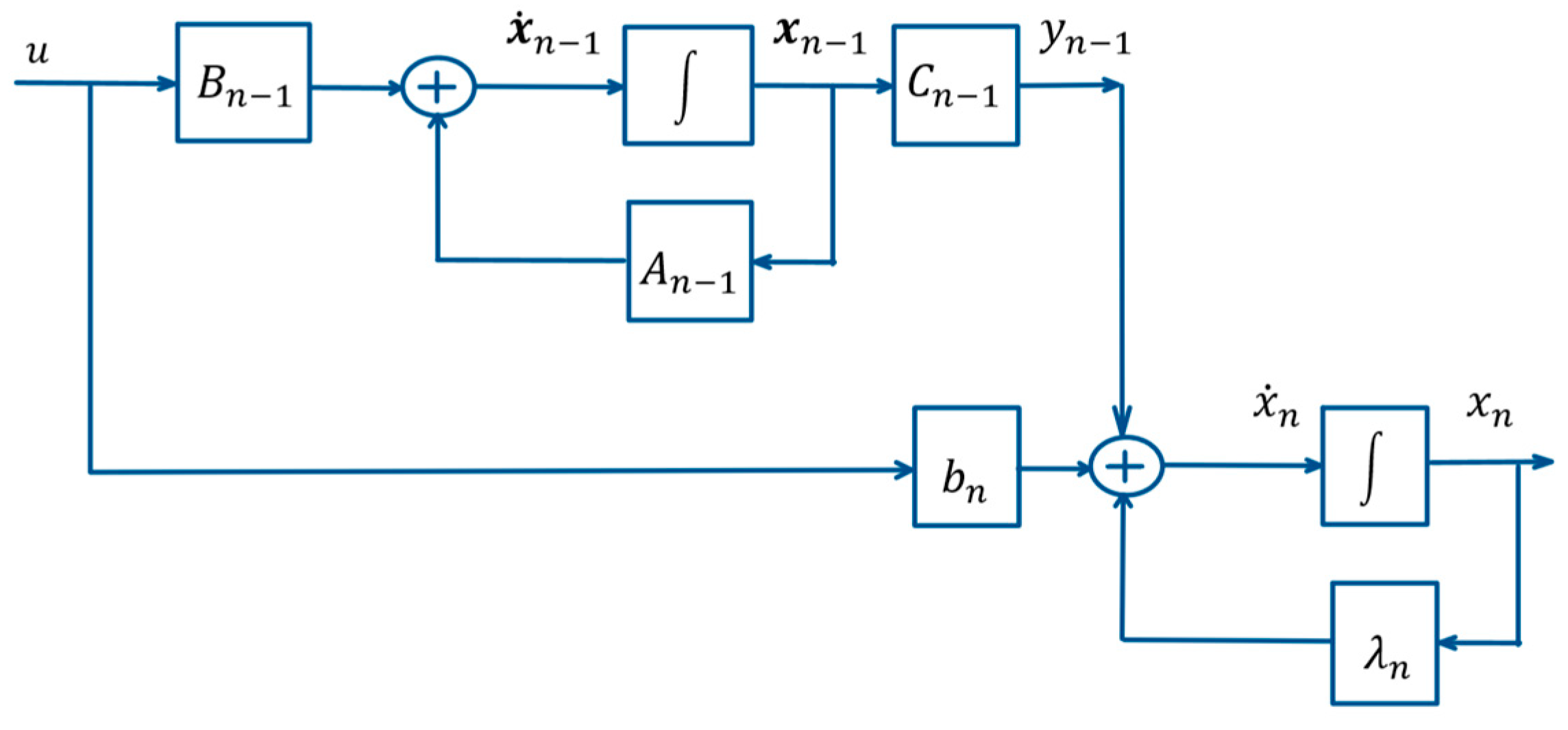
The form of the system (1) allows the introduction of the linear sub-system (7) of order with a state-space vector, (8), and a scalar output, , by the matrices (9). Thus, the system (1) can be represented by (7) in the form (10), which is also depicted in Figure 1. With regard to the sub-system (7), its initial state represents (11) and the relation between the initial state (2) of the system (1) and the initial state (11) of the sub-system (7) represents (12).

Figure 1.
Schematic representation of the initial system (1) in form (10).
Let as formulate now the following linear time-optimal control problem of order , which we shall call “Problem P”. The system is represented by Equation (7). The initial state of the system (7) at the moment is (11), and the target state at the moment , which is preliminarily unspecified, is the origin (13) of the -dimensional state-space of the system (7). The admissible control represents a piecewise continuous function that takes its values from the range (3), which is continuous on the boundaries of the set of allowed values (3), and at the points of discontinuity we have (4). Problem P consists of synthesizing an admissible control that transfers the system (7) from its initial state (11) to the final state (13) and minimizes the performance index (14).
Let us assume we have found the solution of Problem P and denote by the optimal time—the minimum time (15) of (14), by the optimal control, and by the optimal trajectory in the -dimensional state-space of the system (7), which is described by (16) and (17).
Let us denote the scalar output of the system (7) in case it is the result of the optimal vector function as . In that case, is represented by (18) and (19).
In [20], the following theorem has been proven.
Theorem 1.
The trajectory of the system (1) or (10) with an initial point in (2) under the optimal control, of Problem P lies wholly on the switching hyper-surface of Problem P and ends at the moment at the origin of the -dimensional state space of the system (1) or (10) of Problem P, or lies entirely above or below the switching hyper-surface of Problem P nowhere intersecting it and ends at the moment at a point of the coordinate axis different from zero.
The theorem above plays an essential role in the further consideration of this problem. Let us present some elements of its derivation.
First, a vector function, , with an initial point representing the initial state (2) or (12) of Problem P under the optimal control of Problem P is considered. The following expression is obtained for it:
At the second step, a special initial point, , in the -dimensional state space of the system of Problem P is formed:
The first ) coordinates of the initial state above and the first ) coordinates of the initial state (2) of Problem P are the same and are practically the initial state (11) of the generated sub-problem, Problem P.
At the third step, the trajectory in the -dimensional state space of Problem P() with an initial state at point under the optimal control of Problem P is formed. The result is:
We have determined that the trajectory in the -dimensional state-space of the system (1) or (10) with initial point (21)–(22) under the optimal control of Problem P() ends at the moment at the origin of the -dimensional state space of Problem P(). Taking into account that the function is the optimal control of Problem P() and thereby it represents a piecewise constant function with the maximum amplitude, , and number of switchings (), i.e., with the number of intervals of constancy maximum () [7] (Chapter 2, §6, Theorem 2.11, p. 116), the trajectory, , lies wholly on the switching hyper-surface of Problem P().
At the fourth step, the difference between the vector functions above, (20) and (23), is considered. We show that:
Let us cite the corollaries obtained in the discussion of the above result:
As for the last -th coordinate of (31) of for , we can state that:
- If , then the initial state (2) or (12) of Problem P() coincides with point with coordinates (21)–(22). As already illustrated, represents a point of the switching hyper-surface of Problem P(), and the trajectory with the initial point under the optimal control of Problem P() lies wholly on the switching hyper-surface of Problem P() and ends at the moment at the origin of the -dimensional state space of the system (1) or (10) of Problem P();
- If , then the initial state (2) or (12) of Problem P() does not coincide with point with coordinates (21)–(22). The expression for does not change its sign and is not equal to zero because is a finite time. Thus, the trajectory with initial state (2) or (12) of Problem P() under the optimal control of Problem P() lies entirely above or below the switching hyper-surface of Problem P(), nowhere intersecting it, and ends at the moment at a point of the coordinate axis different from zero [20] (p. 7).
3. Derivation of Some New Properties of the Considered Time-Optimal Control Problem
Let us continue with the consideration of the second case of the expression above (24) with regard to its last -th coordinate for , i.e., when . In case
and sequentially describes all the values of the interval , then by (24), all the points of the line passing through point with coordinates (21)–(22) parallel to the axis and located above point by (24) are transformed at the moment successively into the points of the positive part of the axis of the -dimensional state space of Problem P, whereby all these trajectories are located outside the switching hyper-surface of Problem P having one and the same relation to it, simultaneously above or simultaneously below the switching hyper-surface of Problem P. Thus, the positive semi-axis is outside the switching hyper-surface of Problem P, being wholly below or wholly above the switching hyper-surface of Problem P. When
based on the same reasoning, we see that the negative semi-axis is outside the switching hyper-surface of Problem P, being wholly below or wholly above the switching hyper-surface of Problem P, but in the opposite relation to the switching hyper-surface of Problem P relative to the positive semi-axis Based on this conclusion, for the considered class of problems, we can define the term for the variable .
Definition 1.
We define as a variable taking only one possible value, or , i.e.,
so that, for the optimal control of Problem P
is satisfied.
In order to determine , let us now perform the following few constructions.
3.1. Construction 1
First, let us first choose random positive finite numbers , , …, , i.e.,
Let us form the following piecewise constant function, , as an admissible function for the considered class of problems, where its value in the -th interval, , is
Note that the value of in the first interval of constancy is .
Let us denote by the length of the function or the sum of the lengths of all intervals of constancy of
Let the initial state of Problem P be the following point in the -dimensional state space of Problem P
Let us now consider the trajectory in the -dimensional state space of Problem P with an initial state (32) under the control (30)
It is easily seen that the control (30) transfers the initial state (32) of the system (7) of Problem P at the moment at the origin of the -dimensional state space of Problem P:
Thus, we can draw the following conclusion.
Corollary 1.
The piecewise constant function (30) with an amplitude of , non-zero intervals of constancy , , …, , and a value in the first interval of constancy transfers the system of Problem P from its initial state (32) at the final moment (31) at the origin of the -dimensional state space of Problem P The function represents the optimal control of Problem P with an initial state of the system . The point is located outside the switching hyper-surface of Problem P.
Let us denote by the output of the system (7) of Problem P with an initial state (32) under the control (30) for
3.2. Construction 2
Secondly, let us now consider Problem P with an initial state of the system (1) in form (10) at the point with coordinates
where is (32), is (38), is (30), but (41) is the initial state of the -th coordinate of the state-space vector of the system (1) or (10). Let us consider the trajectory in the -dimensional state space of Problem P with an initial state at the point with coordinates (40) and (41) under the control (30), which, according to Corollary 1, represents the optimal control of Problem P with an initial state (32). The vector function based on the representation of the system (1) in form (10) is described as
For the state at the moment :
bearing in mind (34)–(37) and replacing with the expression for it (41), we obtain consecutively:
Thus, we can draw the following conclusion.
Corollary 2.
The trajectory in the -dimensional state space of the system (1) or (10) with an initial point (40) and (41) under the control (30) ends at the moment at the origin of the -dimensional state space of Problem P. Taking into account Corollary 1, where the function is a piecewise constant function with an amplitude and exactly intervals of constancy, and represents the optimal control of Problem P, whose purpose-built initial state is generated also as initial state of the sub-problem by the initial point, (40), of Problem P, then it follows that, in accordance with [7] (Chapter 2, §6, Theorem 2.11, p. 116), the trajectory lies wholly on the switching hyper-surface of Problem P. The value of the optimal control for this point, , is , as the control in the first interval of constancy of . The point is a point from the manifold according to the exposition in Section 1 based on Pontryagin’s original sources [1] (Chapter 3, § 20, § 21, Example 3).
3.3. Construction 3
Let us employ the matrix representation of Equation (1) of the original system of Problem P and the relation by the form (10) with the system (7)–(9) of order of its sub-problem Problem P, a matrix representation of which is also depicted in Figure 1.
Let be an arbitrary positive number, i.e.,
and consider the state in the -dimensional state space of the system of Problem P with coordinates
as well as the trajectory starting at this point under the constant control when
The final point of this trajectory at moment is the state (40)–(41) in the -dimensional state space of the system of Problem P.
We see that the points of the trajectory starting at under the control fall into point , which is a point from the switching hyper-surface of Problem P Keeping in mind Corollary 2 and following Pontryagin [1] (Chapter 3, § 20, § 21, Example 3), we can draw the following conclusion.
Corollary 3.
The entire trajectory, (55), with an initial point (54) under the constant control with a duration , ending at (40)–(41), but without the endpoint itself is a part of the manifold , which is the part of the state space of Problem P outside the switching hyper-surface of Problem P with a value of of the optimal control for the points of this manifold.
Briefly stated, the points of the manifold are above the switching hyper-surface of Problem P, while the points of are below the switching hyper-surface of Problem P.
Let us form the following piecewise constant function, , with intervals of constancy, where the duration of the first interval is and the value of the function there is , while from the second till the -th interval, the function represents the shifted-to-the-right by a distance function (30), i.e., the duration of the second interval is while the value there is and so on for the intervals after the second one till the -th one, which is with a length and a value of the function within it . We can describe the function in the following two ways.
Then, the point (54) in the -dimensional state space of the system of Problem P expressed in (54) by (40) and (41) is also expressed as:
Corollary 3 can be amended with the following corollary.
Corollary 4.
The piecewise constant function , , (60) or (61) with non-zero intervals of constancy represents the optimal control of Problem P with an initial state (62) or (54).
3.4. Construction 4
Let us now consider Problem P with an initial state (62) or (54) and its respective sub-problem Problem P. Let us form the trajectory in the -dimensional state space of the system of Problem P with an initial state under the optimal control of Problem P:
According to Corollary 3 and 4, . Therefore, in Theorem 1, this trajectory also lies in —lies above the switching hyper-surface of Problem P, nowhere intersecting it and ends at the moment at a point of the coordinate axis different from zero.
Considering the relation (12) between the initial state (2) of Problem P and the initial state (11) of Problem P:
the trajectory (63) according to (20) represents:
The final point of this trajectory lies on the axis :
Thus, the value, more precisely, the sign of the last -th coordinate
indicates whether the positive or negative part of the axis is a part of the manifold , i.e., is above the switching hyper-surface. We obtain
Thus, if , then the positive part of the axis is a part of the manifold , i.e., is located above the switching hyper-surface, and accordingly the negative part of the axis is below the switching hyper-surface or is a part of the manifold .
When , then the negative part of the axis is a part of the manifold , i.e., is located above the switching hyper-surface, while the positive part of the axis is below the switching hyper-surface or is a part of the manifold .
Thus, the following theorem with regard to the “axes initialization” has been proven.
Theorem 2.
If (62) is the initial state of Problem P, where , , …, are random finite positive numbers, the function , is a piecewise constant function with non-zero intervals of constancy (61) with an amplitude of , and starts with a value on its first interval, then:
- The point and the function , represent the optimal control of Problem P;
- The trajectory (63) in the -dimensional state space of the system of Problem P with an initial point, , under the optimal control of Problem P is also located in the manifold —lies above the switching hyper-surface of Problem P, nowhere intersecting it and ends at the moment at the point (67) of the coordinate axis different from zero;
- The sign of this -th coordinate (69) indicates whether the positive or the negative part of the axis is a part of the manifold i.e., is above the switching hyper-surface. Thus, if , then the positive part of the axis is a part of the manifold , i.e., is located above the switching hyper-surface, and accordingly the negative part of the axis is below the switching hyper-surface or is a part of the manifold . When , then the negative part of the axis is a part of the manifold , i.e., is located above the switching hyper-surface, while the positive part of the axis is below the switching hyper-surface or is a part of the manifold .
3.5. Construction 5
Let us now consider Problem P with an initial state at the point , which can now be any point in the -dimensional state space of the system of Problem P Suppose that we have solved the simpler sub-problem Problem P and obtained of Problem P Let us consider the trajectory in the -dimensional state space of the system of Problem P with an initial point under the optimal control of Problem P:
Based on the relation (12) between the initial state (2) of Problem P and the initial state (11) of Problem P
the trajectory (70) according to (20) is described as:
The final point of this trajectory, , lies on the :
According to Theorem 1, this entire trajectory, (70) or (72), i.e., all its points, have the same relation to the switching hyper-surface of Problem P. Let us now consider the possible cases.
Case 1. The trajectory lies entirely on the switching hyper-surface of Problem P, and the final point at the moment is the origin of the -dimensional state space of the system of Problem P. Therefore, the -th coordinate of (74) is also 0:
In this case, the optimal control —the solution of the sub-problem Problem P, which is a piecewise constant function with at most intervals of constancy, i.e., with at most switchings, is also the solution of Problem P:
Case 2. The trajectory lies wholly above or below the switching hyper-surface of Problem P, nowhere intersecting it, and the final point at the moment is a point of the coordinate axis different from zero. Therefore, the -th coordinate of (74) satisfies:
Case 2.1. If the sign of the specified -th coordinate above and the sign of the variable (69) are the same, then according to the proved Theorem 1, the entire trajectory, (70) or (72), belongs to the manifold , i.e., all the points of are points of the manifold or are located above the switching hyper-surface of Problem P:
Case 2.2. If the sign of the specified -th coordinate and the sign of the variable (69) are opposite to each other, then according to the proved Theorem 1, the entire trajectory, (70) or (72), belongs to the manifold , i.e., all the points of are points of the manifold or are located below the switching hyper-surface of Problem P:
Let us define the variable , which is the value of the -th coordinate of the final state (74) of the trajectory, (70) or (72), obtained under the optimal control of Problem P at the moment in the -dimensional state space of the system of Problem P with an initial state :
Thus, the following theorem with regard to the synthesis of the time-optimal control at the initial state of Problem P has been proven.
Theorem 3.
If the optimal control of the sub-problem Problem P is found—the solution then the optimal control at the initial state of Problem P can be determined as:
The following consequence of Theorem 2 holds.
Consequence 1.
In the case that
, then the solution of Problem P
represents the already found solution of the sub-problem Problem P:
Let us consider the case when . This means that the initial state of the system of Problem P is outside the switching hyper-surface of Problem P, i.e., it is a point of the manifold , , or In this case, assume that the optimal control at the initial state of Problem P and the optimal control at the initial state of Problem P are the same, i.e., both have the value or simultaneously:
It follows from the above that the optimal control of Problem P as a piecewise constant function with at most intervals of constancy with an amplitude has at least one interval of constancy. Let us denote its length as . So, it is valid:
Let us consider the trajectory (70) or (72) in the -dimensional state space of the system of Problem P with an initial state obtained under the optimal control of the sub-problem Problem P. According to Theorem 1, this trajectory, (70) or (72), lies entirely in one of the two manifolds or of the state space of Problem P Let us consider the first section of this trajectory formed under the constant control with a value and a duration :
Then, the first section of the trajectory, (70) or (72), for in the -dimensional state space of the system of Problem P is described as:
Since (83) is fulfilled in this case, then for (86) or the first section of the trajectory, (70) or (72), it is valid that:
The possible options for the optimal control at the point can only be or . If , then , and if , then .
Thus, this section (87) of the trajectory (70) or (72) in terms of is:
But (88) describes the part of the optimal trajectory of the system in the manifold of the -dimensional state space of the system of Problem P with an initial point obtained under the optimal control for the points of this manifold for in the case when while (89) describes the part of the optimal trajectory of the system in the manifold of the -dimensional state space of the system of Problem P with an initial point obtained under the optimal control for the points of this manifold for in the case when . Thus, we proved the following corollary of Theorem 2.
Consequence 2.
When and , then the first section of the trajectory in the -dimensional state space of the system of Problem P with an initial point obtained under the optimal control of the sub-problem Problem P and formed under the constant control with a value and a duration , in addition to being outside, above or below and nowhere intersecting the switching hyper-surface of Problem P, is also a part of the optimal trajectory of Problem P located in the manifold when or located in the manifold when
4. Examples
4.1. Example 1
Let us consider the following already classical example of synthesizing the time-optimal control of a double integrator [7] (§ 3. Example. The problem of synthesis, p. 38), [10] (Chapter 7, Problem 7.1, p. 150) [11]. This example found a place in online optimal control courses on world platforms with video content [21,22,23,24]. To illustrate in [20] the extension of the main ideas of the proposed method, we have already partially used this example there. Precisely because this example is quite popular, our aim is to demonstrate on it the new technique in its entirety. This includes first the axes initialization stage based on Theorem 2 and then the synthesis stage based on Theorem 3 to obtain time-optimal trajectories of the double-integrator system.
The system of a double integrator is represented in (90). For convenience, in terms of a mechanical system, we can denote the variable as the position and as the velocity. Let the constraints of the admissible control (3), (4) be (91).
First, let us make a suitable change in variables and by and , respectively, as presented in (92), and obtain a representation of the initial system (90) by in the form (1) following the technique in [20] (pp. 9–10). We successively obtain:
The system (98) is now in the form (1) of the system of the original Problem P( when Then, (98) in form (10) is represented as (99)–(100) (as (1) in form (10)). The sub-system of (99)–(100) is (101) or (102).
4.1.1. Axes Initialization
Let us carry out an “axes initialization” for Problem P( above with equations of the system (99)–(100) and equations of the system of the sub-problem Problem P (101) or (102).
The fact that is simply stated in the example of [20] (p. 11). We will derive this result based on the theoretical conclusions obtained here.
For , according to Construction 1, we choose an arbitrary finite positive (29), for example
The piecewise constant function (30), in this case with only one interval of constancy with a length (103), represents
The duration of is
We obtain for the initial state (32) of Problem P, here in the one-dimensional state space of Problem P:
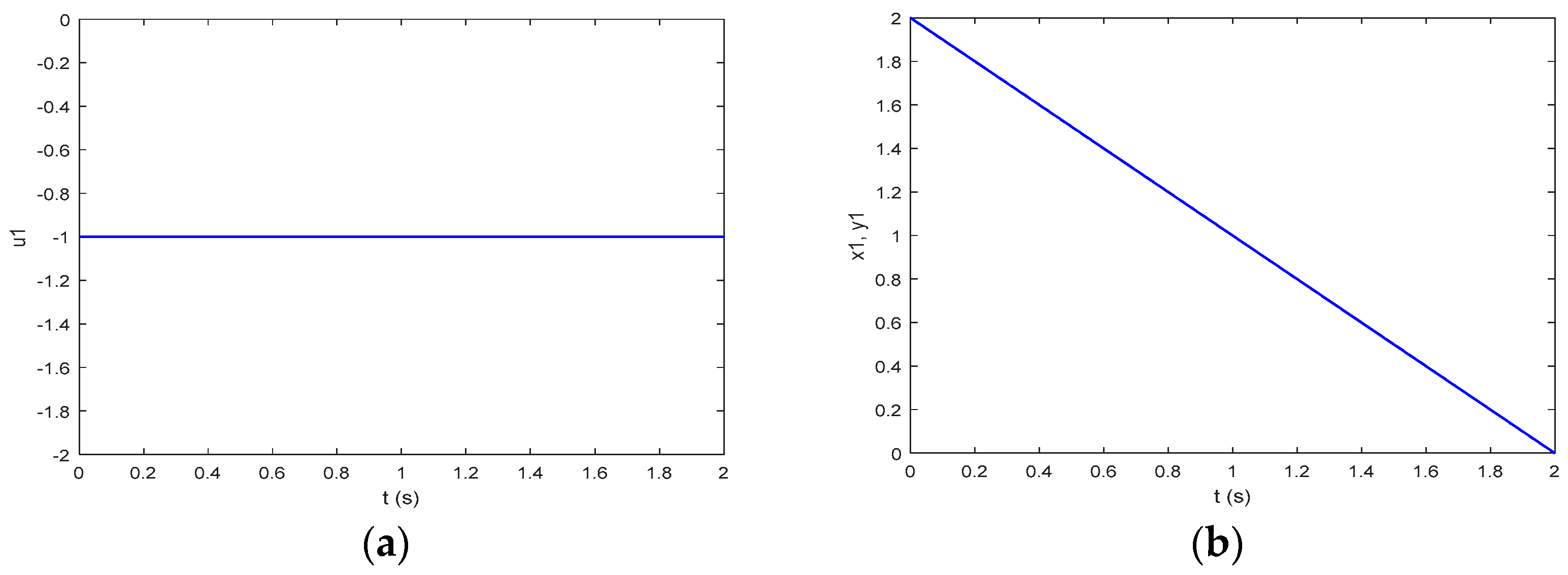
Figure 2 shows the transition from the initial state above, , of the system of Problem P to the one-dimensional state-space origin under the control (104) with a duration (105), which is an illustration of Corollary 1 of Construction 1. Since , the output of the system of Problem P (38) is and coincides with , the state here.
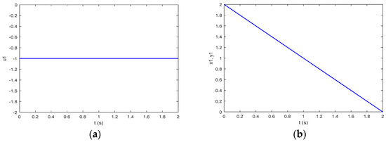
Figure 2.
The purpose-built function (103)–(105) and the resulting time-optimal process of the system of Problem P(1): (a) the control ; (b) the state and the output of the system of Problem P(1).
We obtain for the point (40) by Construction 2:
where the coordinate (41), in this case , is
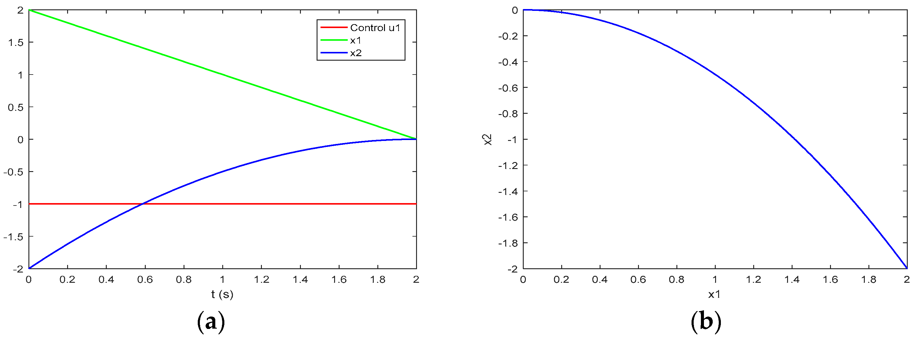
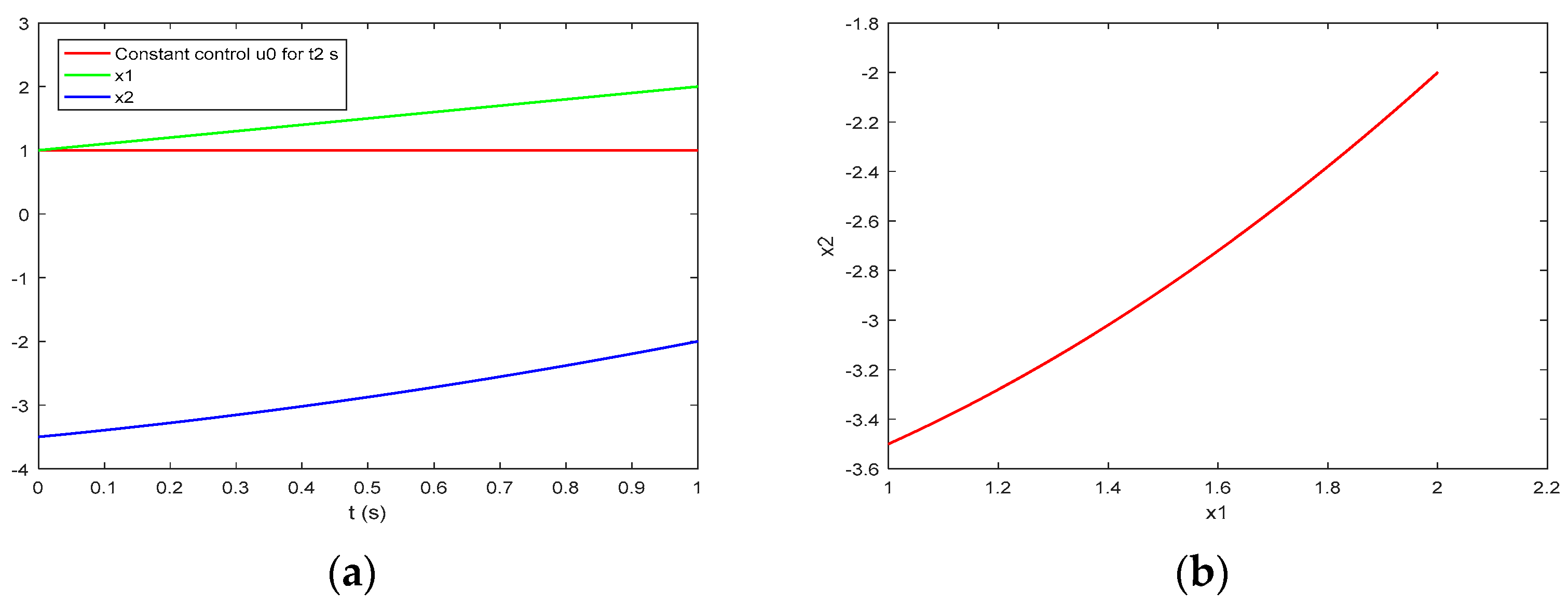
Figure 3 illustrates Corollary 2 of Construction 2. Figure 3a depicts the process of the system of Problem P with an initial state at the point (107) under the control (104), (105). The process in the phase plane of the system of Problem P is depicted in Figure 3b, and this phase trajectory is a part of the manifold .
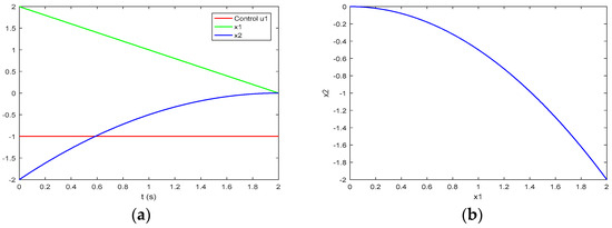
Figure 3.
The movement in the manifold of Problem P from the obtained initial state (107), for which the control (103)–(105) is the time-optimal one: (a) the process and the control ; (b) the phase trajectory in .
Let us proceed to Construction 3. We now choose , in our case , as an arbitrary finite positive number according to (53). Let, for example,
For the point (54), we obtain
As an illustration of Corollary 3 of Construction 3, Figure 4a shows the process of the system of Problem P with an initial point (110) under the constant control for transferring the system at the point (107). The phase trajectory is depicted in Figure 4b. This trajectory without the final point (107) is a part of the manifold , while the final point (107) belongs to the manifold .
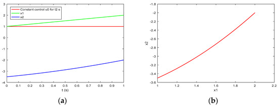
Figure 4.
The trajectory of the system of Problem P with a duration s from the initial state (110) in the manifold until entering the manifold at the state (107): (a) the process itself; (b) the phase trajectory in .
Let the piecewise constant function with intervals of constancy be formed according to Construction 3 in the way (61):
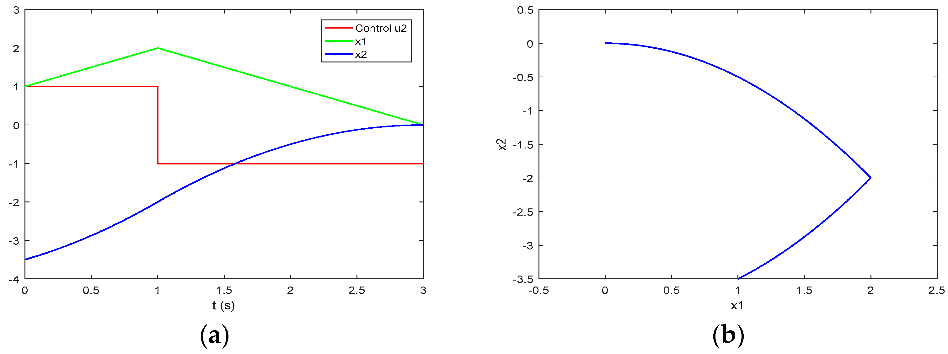
Figure 5a shows the process of the system of Problem P with an initial point (110) under the piecewise constant function (111), while in Figure 5b, the respective trajectory in the phase plane is depicted. The first section of the trajectory from the point (110) until the state (107), but without the final point itself, is in the manifold , while the second section starting at (107) till the state-space origin is a movement lying in the manifold or on the part of the switching hyper-surface formed under the control . According to Corollary 4 of Construction 3, the piecewise constant function , ], (111) with two non-zero intervals of constancy is the time-optimal control of Problem P with an initial state at the point (110).
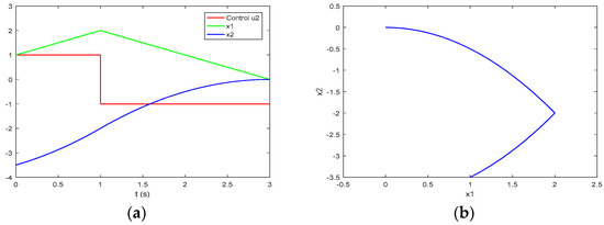
Figure 5.
The optimal process of the system of Problem P with the derived initial state (110) for which the time-optimal control is the specially constructed function (103), (109), (111): (a) the process; (b) the trajectory in the phase plane .
Let us proceed to Construction 4. We form the sub-problem Problem P of Problem P with an initial state, (54), which in this case is the obtained point (110). The equations of the system of Problem P are (102), and the initial state of Problem P derived from (110) is:
The solution of Problem P according to [20] (p. 10) is:
We obtain in our case:
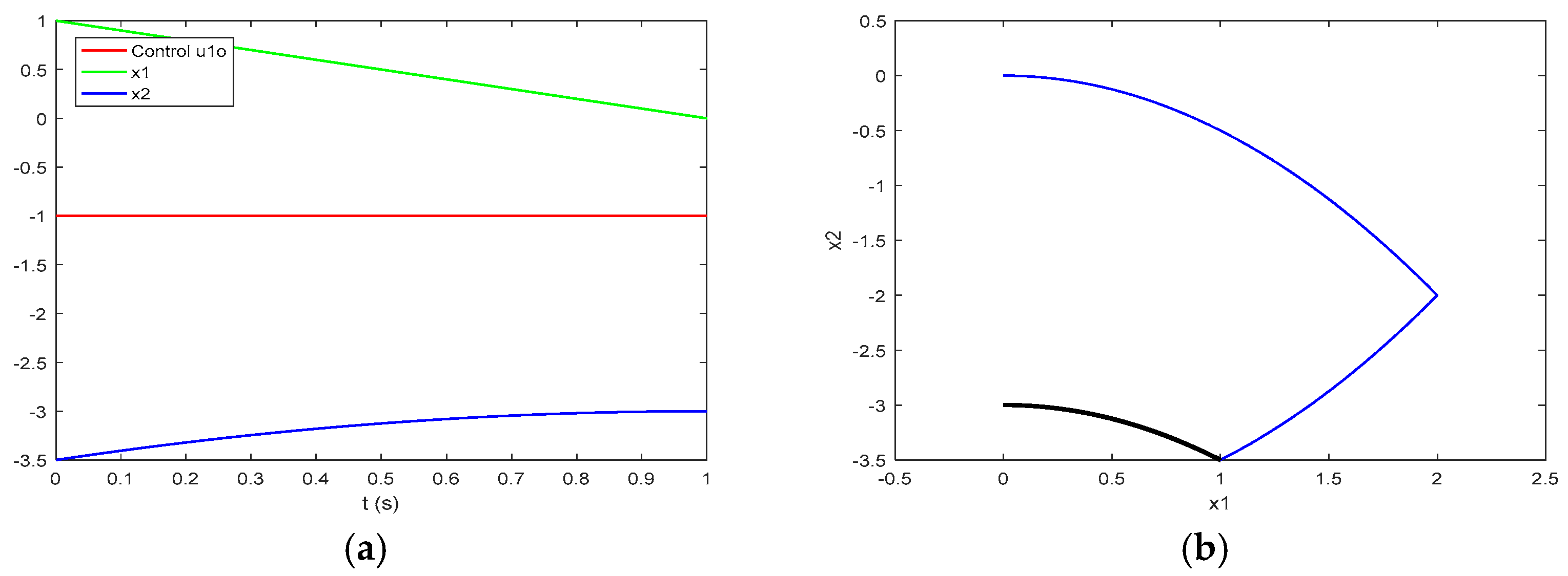
Figure 6a presents the process of the system of Problem P with an initial state at the point (110) under the piecewise constant function with one interval of constancy and a value which is the solution of Problem P. The process in this case corresponds to the process (63) or (65) of Construction 4. The black trajectory in Figure 6b shows the respective trajectory in the phase plane of Problem P, while the blue one outlines the trajectory from the same initial point (110) but obtained under the piecewise constant function , ] (111), and also shown in Figure 5b. The final point of this process , which corresponds to the final point (67) of (63) or (65), is:
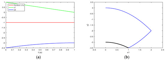
Figure 6.
Trajectories of the system of Problem P with an initial state (110): (a) the process under the optimal control of the sub-problem Problem P; (b) marked with black, the phase trajectory corresponding to the process in (a), and the optimal phase trajectory for the point marked with blue.
That is a point on the axis , in this case different from the state-space origin. The sign of the value of the last coordinate, the second coordinate here, of this point indicates which part of this axis belongs to the manifold . Following (69), we obtain:
Thus, according to Theorem 2 for , the negative part of the axis, , belongs to the manifold i.e., is located above the switching hyper-surface, while the positive part of the axis, , is below the switching hyper-surface or is a part of the manifold .
4.1.2. Synthesis of the Time-Optimal Control
Let us now illustrate the synthesis of the time-optimal control and Consequence 2 of Theorem 3. For this purpose, let the initial state of Problem P be:
The sub-problem Problem P in this case is with an initial state
We use the already known solution of Problem P with this initial state (121) or (112). For the variable (80), in our case , we obtain successively:
For oblem P according to Theorem 3 by (81), taking into account (119), we obtain:
It follows from the result above and the solution (116)–(117) of Problem P that:
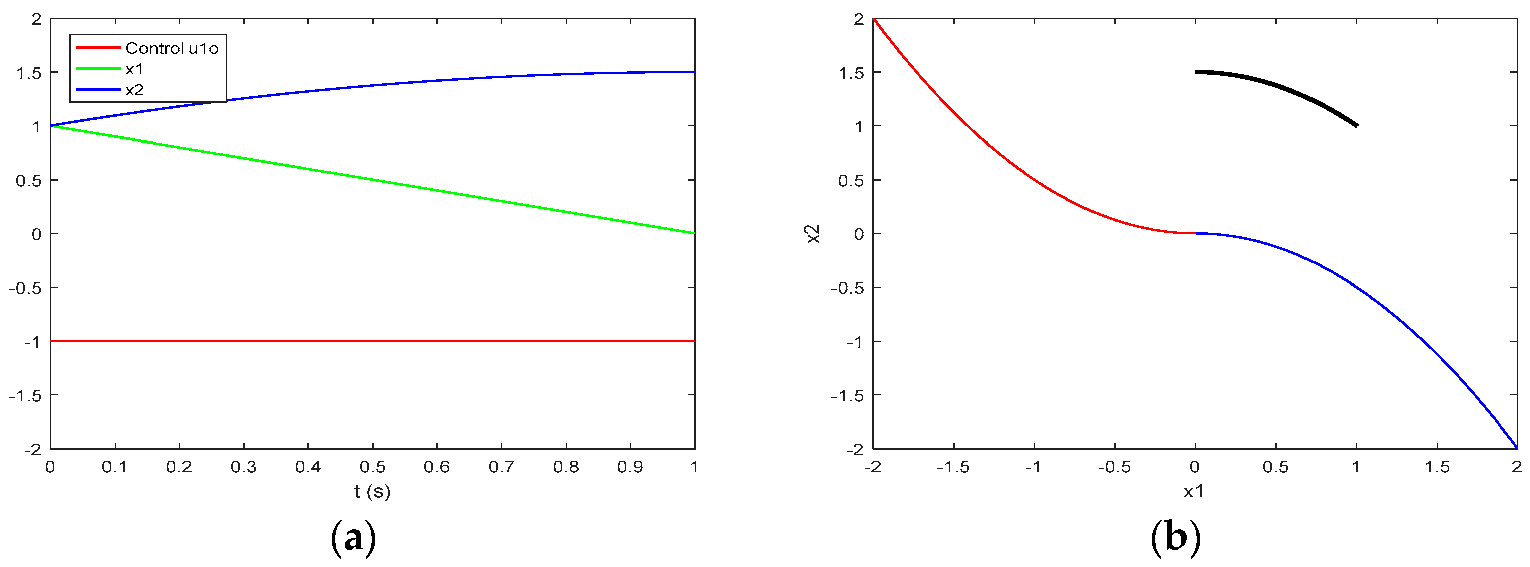
Thus, according to Consequence 2 of Theorem 3, the first section of the trajectory in the phase plane of Problem P with an initial state (120) obtained under the optimal control (116)–(117) of Problem P, in addition to being outside, above or below, nowhere intersecting the switching curve, the manifold of Problem P, is also a part of the optimal trajectory of Problem P located in the manifold This relation is also shown in Figure 7b, where the black trajectory concerns the phase trajectory under the optimal control (116)–(117) of Problem P, the manifold is marked with blue, the manifold is marked with red, and the switching curve is . The process of the system of Problem P with an initial state formed under the control (116)–(117) is depicted in Figure 7a.
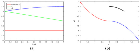
Figure 7.
The trajectory of the system of Problem P with an initial point obtained under the control (116)–(117): (a) the process itself; (b) the trajectory in the phase plane of Problem P.
Figure 8a shows the near time-optimal process of Problem P with an accuracy . The green trajectory in Figure 8b outlines the corresponding trajectory in the phase plane of Problem P. It covers the black phase trajectory obtained under the optimal control (116)–(117) of the sub-problem Problem P, which is also shown in the previous Figure 7b. The manifold presented in blue, and the manifold presented in red, are also shown in this Figure 8b. The switching curve is .
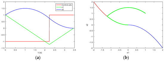
Figure 8.
The near-time-optimal trajectory of the system of Problem P referring to the initial state with an accuracy of : (a) the near-time-optimal process; (b) the trajectory marked with green in the phase plane of Problem P alongside the manifold marked with red and blue.
4.2. Example 2
Let us now consider the following time-optimal control problem for a hypothetical system of order seven with the data:
On the basis of Problem P according to the relations (49)–(52), the set “Problem P, Problem P, …, Problem P, Problem P” is established.
Let us set for a given accuracy, , a hyper cube around the state-space origin and assume that the terminal state for a given problem can be any point in the corresponding area. We consider an admissible control as an approximate problem solution, a near-time-optimal solution with an accuracy of if it is the optimal control making possible to reach a terminal state within the established area.
Let us denote the approximate solutions for the class of problems P, P, …, P by and for . The control functions are piecewise constant functions with no more than non-zero intervals of constancy with lengths and signs , respectively.
After the first axes’ initialization stage, the following set for the variables , , …, is obtained:
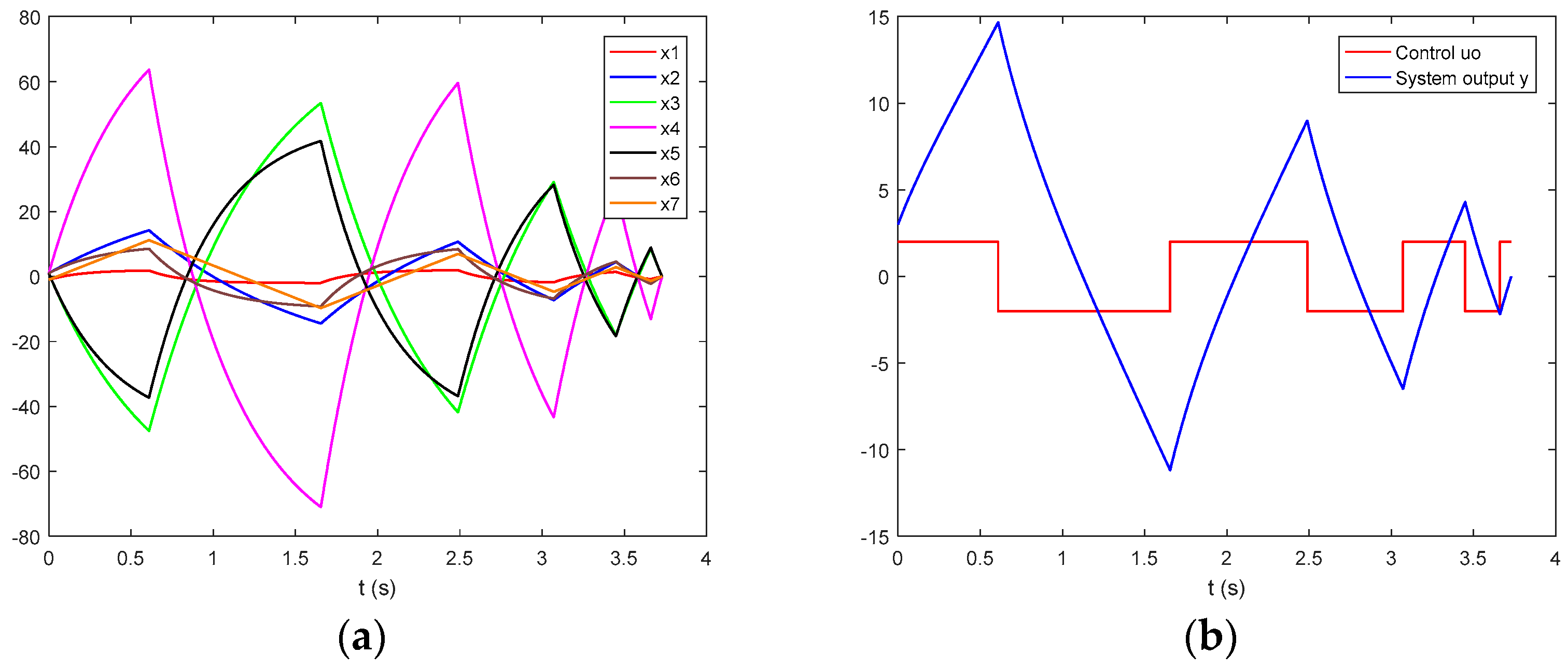
An approximate problem solution with an accuracy of is computed using the proposed technique for time-optimal control synthesis. The results are presented in Table 1 and Figure 9. The system output
is also shown in Figure 9.

Table 1.
Results of an approximate solution of Problem P with an accuracy of .
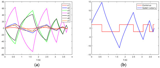
Figure 9.
An approximate time-optimal process of Problem P from the initial state to the origin of the state space with an accuracy of : (a) the near-time-optimal process with respect to the state-space variables; (b) the respective approximate time-optimal control and the system output .
Let us consider now Problem P, but with an initial state
According to the results (130) of the axes initialization, . So, the negative part of the axis belongs to the manifold , i.e., is located above the switching hyper-surface of Problem P while the positive part of the axis belongs to the manifold . Thus, the time-optimal control at the initial state (132) of Problem P is
and represents a piecewise constant function with just seven intervals of constancy or with just six switchings.
We can obtain (133) also applying Theorem 3. The initial state of the sub-problem P bearing in mind the relation (12) represents
This means that the initial state coincides with the final state of Problem P representing the state-space origin of the system of Problem P. Therefore, we can formally represent the length of the time-optimal control function of Problem P as
The calculated value of the variable , in our case , needed in (81) for Theorem 3, in accordance with (80) represents
Thus, we obtain according to Theorem 3:
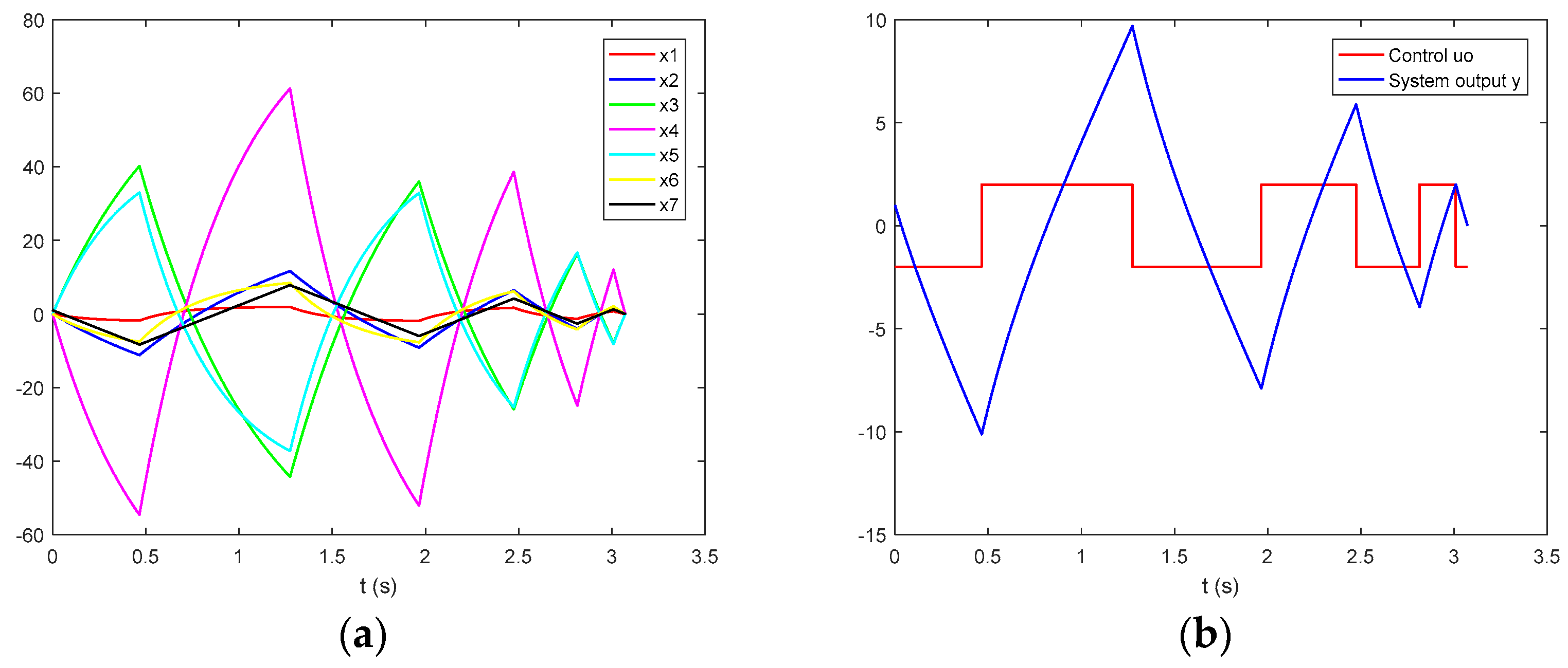
The results of an approximate problem solution with an accuracy of are presented in Table 2 and Figure 10. The number of non-zero intervals of constancy of the function is seven.
Table 2.
Results of an approximate solution of Problem P with an initial state (132) and an accuracy of .
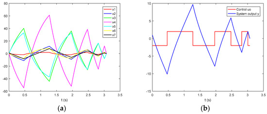
Figure 10.
An approximate time-optimal process of Problem P from the initial state to the origin of the state space with an accuracy of : (a) the near-time-optimal process with respect to the state-space variables; (b) the respective approximate time-optimal control and the system output .
5. Concluding Remarks
Example 2 shows that the solution of the time-optimal control problem based on the considered method in the case of the system order being higher than two includes generating from the original Problem P the sub-problems Problem P, …, Problem P, Problem P. Every single problem of the set “Problem P …, Problem P” requires an axes initialization, in order to determine the respective value of for the considered Problem P and obtaining the set , , …, . A feature here is to obtain this set starting from and by successive ascent reaching the original highest order, .
Obtaining by Theorem 3 the optimal control for a given initial state is based on the solution of the corresponding sub-problem. Consequences 1 and 2 are the theoretical bases for an accelerated solution of all sub-problems of the original Problem P by jumping in certain cases along the optimal trajectories of these sub-problems without the need for internal movement along them. This further reduces the computational load that has already been reduced based on the preliminary knowledge of the corresponding state spaces of Problem P to Problem P through the axes initialization and the subsequent synthesis based on the solution of the generated lower-order lighter sub-problem relative to the original one.
It is easily seen that, in case of the second-order system, such jumps while moving continuously along the optimal trajectory are not possible. However, in the case of a third-order system or higher, such jumps when the lower-order time-optimal control problem is invoked, are absolutely reasonable and accelerate the synthesis process of the higher-order problem.
On the other hand, it is also easily seen that the spared computing time depends on the initial state of the invoked problem. At the time of presenting the theoretical findings here, a software has not yet been developed to implement the new method in its entirety for higher-order systems also including such estimations. The numerical aspects arising in higher-order systems in the implementation of the method are a matter of special study.
One might say that the results obtained here sound similar to some previous works, but this is not exactly the case. A detailed tracing of the evolution of the idea shows the following main distinctive features of the current results. The first feature concerns the basic fact that the properties here completely cover the case of the theorem about the number of switchings or the number of intervals of constancy and differ from the narrower case of simple and non-negative eigenvalues of the system. The second feature concerns the derivation technique here, which is much more elegant and different from the previously adopted approach involving some properties of certain systems of linear differential equations under the piecewise constant control function [14] of [20] (Chapter 2, pp. 16–27), [15] of [20] (p. 319), [16] of [20] (pp. 42–45). The previous paper [20] and the current work are examples of how a seemingly small property of a problem can be developed into a rigorously proven method by the research from the particular to the general and discovering subsequent properties contributing in our case to the state-space analysis of the linear time-optimal control problem following from Pontryagin’s maximum principle.
There exists a natural interest to know how the proposed design performs under different types of time delay, saturation, and uncertainties, which are very important in the practical industrial context [25]. These issues form a bridge between the anti-windup and override feedback schemes [26,27,28]. These topics deserve special study, bearing in mind the potential of the proposed design to deal with higher-order systems and possibly reduce the computational load.
Funding
This research was funded by the European Regional Development Fund under the Operational Program “Scientific Research, Innovation and Digitization for Smart Transformation 2021–2027”, Project CoC “Smart Mechatronics, Eco- and Energy Saving Systems and Technologies”, BG16RFPR002-1.014-0005.
Data Availability Statement
Data are contained within the article.
Acknowledgments
The author would like to thank the Project CoC “Smart Mechatronics, Eco- and Energy Saving Systems and Technologies”, BG16RFPR002-1.014-0005, for the financial support.
Conflicts of Interest
The author declares that he has no conflicts of interest.
References
- Pontryagin, L.S.; Boltyanskii, V.G.; Gamkrelidze, R.V.; Mischenko, E.F. The Mathematical Theory of Optimal Processes; Pergamon Press: Oxford, UK, 1964. [Google Scholar]
- Feldbaum, A.A. The simplest relay automatic control systems. Autom. Remote Control. 1949, X, 5. (In Russian) [Google Scholar]
- Feldbaum, A.A. Optimal processes in automatic control systems. Autom. Remote Control. 1953, XIV, 6. (In Russian) [Google Scholar]
- Athans, M.; Falb, P.L. Optimal control. In An Introduction to the Theory and Its Applications; McGraw-Hill: New York, NY, USA, 1966. [Google Scholar]
- Lee, E.B.; Markus, L. Foundations of Optimal Control Theory; Wiley & Sons Inc.: Hoboken, NJ, USA, 1967. [Google Scholar]
- Bryson, A.E.; Ho, Y.C. Applied Optimal Control; Blaisdell Publishing Company: Waltham, MA, USA, 1969. [Google Scholar]
- Бoлтянский, В.Г. Математические Метoды Оптимальнoгo Управления; Наука: Moskow, Russia, 1969. [Google Scholar]
- Leitmann, G. The Calculus of Variations and Optimal Control; Plenum Press: New York, NY, USA, 1981. [Google Scholar]
- Pinch, E.R. Optimal Control and the Calculus of Variations; Oxford University Press: Oxford, UK, 1993. [Google Scholar]
- Locatelli, A. Optimal Control of a Double Integrator; Studies in Systems, Decision and Control; Springer: Cham, Switzerland, 2017; Volume 68, ISBN 978-3-319-42126-1. [Google Scholar] [CrossRef]
- Romano, M.; Curti, F. Time-optimal control of linear time invariant systems between two arbitrary states. Automatica 2020, 120, 109151. [Google Scholar] [CrossRef]
- He, S.; Hu, C.; Zhu, Y.; Tomizuka, M. Time optimal control of triple integrator with input saturation and full state constraints. Automatica 2020, 122, 109240. [Google Scholar] [CrossRef]
- Consolini, L.; Piazzi, A. Generalized bang-bang control for feedforward constrained regulation. In Proceedings of the 45th IEEE Conference on Decision and Control, San Diego, CA, USA, 13–15 December 2006; pp. 893–898. [Google Scholar] [CrossRef]
- Consolini, L.; Piazzi, A. Generalized bang-bang control for feedforward constrained regulation. Automatica 2009, 45, 2234–2243. [Google Scholar] [CrossRef]
- Consolini, L.; Laurini, M.; Piazzi, A. Generalized Bang-Bang Control for Multivariable Feedforward Regulation. In Proceedings of the 32nd Mediterranean Conference on Control and Automation (MED), Chania, Greece, 11–14 June 2024; pp. 506–511. [Google Scholar] [CrossRef]
- Rustagi, V.; Reddy, V.; Boker, A.; Sultan, C.; Eldardiry, H. Efficient Near-Optimal Control of Large-Size Second-Order Linear Time-Varying Systems. IEEE Control. Syst. Lett. 2023, 7, 3878–3883. [Google Scholar] [CrossRef]
- Qin, C.; Chen, J.; Lin, Y.; Goudar, A.; Schoellig, A.P.; Liu, H.H.-T. Time-Optimal Planning for Long-Range Quadrotor Flights: An Automatic Optimal Synthesis Approach. J. Latex Cl. Files 2021, 14, 8. [Google Scholar] [CrossRef]
- Brunovský, P. The Closed-Loop Time-Optimal Control. I: Optimality. SIAM J. Control. 1974, 12, 624–634. [Google Scholar] [CrossRef]
- Sussmann, H.J. Regular Synthesis for Time-Optimal Control of Single-Input Real Analytic Systems in the Plane. SIAM J. Control. Optim. 1987, 25, 1145–1162. [Google Scholar] [CrossRef]
- Penev, B. One New Property of a Class of Linear Time-Optimal Control Problems. Mathematics 2023, 11, 3486. [Google Scholar] [CrossRef]
- L7.3 Time-Optimal Control for Linear Systems Using Pontryagin’s Principle of Maximum, Graduate Course on “Optimal and Robust Control” (B3M35ORR, BE3M35ORR, BEM35ORC) Given at Faculty of Electrical Engineering, Czech Technical University in Prague. Available online: https://www.youtube.com/watch?v=YiIksQcg8EU (accessed on 15 October 2024).
- Solution of Minimum—Time Control Problem with an Example. Available online: https://www.youtube.com/watch?v=Oi90M3cS8wg (accessed on 15 October 2024).
- Alexandre Girard, Commande Optimale: Exemple Pour le Temps Minimum d’une Masse avec une Limite de Force, Modélisation, Analyse et Commande des Robots, Exemple d’un Calcul de loi de Commande Optimale. Available online: https://www.youtube.com/watch?v=wKjEAXFvXlQ (accessed on 15 October 2024).
- Рютин, К.C. Вариациoннoе исчисление и oптимальнoе управление—12. Задача быстрoдействия. Available online: https://www.youtube.com/watch?v=u7FtLP5BWeg (accessed on 15 October 2024).
- Penev, B.G. Analysis of the possibility for time-optimal control of the scanning system of the GREEN-WAKE’s project lidar. arXiv 2012, arXiv:1807.08300. [Google Scholar]
- Glattfelder, A.H.; Schaufelberger, W. Control systems with input and output constraints; Springer: London, UK, 2003; ISBN 978-1-85233-387-4. [Google Scholar] [CrossRef]
- Hussain, M.; Rehan, M. Nonlinear time-delay anti-windup compensator synthesis for nonlinear time-delay systems: A delay-range-dependent approach. Neurocomputing 2016, 186, 54–65. [Google Scholar] [CrossRef]
- Hussain, M.; Rehan, M.; Ahn, C.K.; Zheng, Z. Static anti-windup compensator design for nonlinear time-delay systems subjected to input saturation. Nonlinear Dyn. 2019, 95, 1879–1901. [Google Scholar] [CrossRef]

Disclaimer/Publisher’s Note: The statements, opinions and data contained in all publications are solely those of the individual author(s) and contributor(s) and not of MDPI and/or the editor(s). MDPI and/or the editor(s) disclaim responsibility for any injury to people or property resulting from any ideas, methods, instructions or products referred to in the content. |
© 2025 by the author. Licensee MDPI, Basel, Switzerland. This article is an open access article distributed under the terms and conditions of the Creative Commons Attribution (CC BY) license (https://creativecommons.org/licenses/by/4.0/).