pth Moment Exponential Synchronization of Fuzzy Stochastic Cellular Neural Networks with Discrete and Infinite Delays

Abstract

In this paper, we consider the pth moment exponential synchronization (PMES) of fuzzy stochastic cellular neural networks (FSCNNs) with discrete and infinite delays. In order to achieve pth-moment exponential synchronization of FSCNNs with discrete and infinite delays, we design an appropriate feedback controller. Using the Lyapunov function method and theories of infinite delayed systems, we obtain some sufficient conditions to ensure the pth-moment exponential synchronization of the system. Finally, to verify the effectiveness of our results, we provide a numerical simulation example. Our results extend the pth-moment exponential synchronization of FSCNNs from finite delays systems to infinite delays systems.

1. Introduction

In recent decades, cellular neural networks (CNNs) have shown their effectiveness in many application domains such as pattern identification [1] and associative memory [2]. In order to optimize the design of CNNs and broaden their practical applications, various dynamic characteristics of CNNs have been thoroughly investigated. In particular, the synchronization behavior of CNNs has been a focus and attracted a lot of research interest in the past few decades [3,4,5,6].

Considering the inherent uncertainty and imprecision in real systems, Yang et al. [7] innovatively integrated fuzzy logic into the traditional cellular neural networks architecture and introduced the concept of fuzzy cellular neural networks (FCNNs) for the first time in 1966. In contrast with conventional CNNs, FCNNs show better ability when performing complex nonlinear filtering tasks, which significantly improves their adaptability and effectiveness in a variety of practical application scenarios. In view of the wide application prospects of FCNNs in many fields, it is particularly important to explore its dynamic characteristics, especially the synchronization behavior [8,9,10].

As the limited information transmission speed will cause a delay effect in the implementation process of neural networks, Roska and Chua [11] integrated the influence of time delays into the fundamental framework of conventional CNNs and pioneered the concept of time-delayed CNNs in 1990. On this basis, Wei et al. [12] further proposed fuzzy logic to address uncertainty and investigated the FCNNs with discrete delays. Moreover, random fluctuations and other variables in the process of neurotransmitter release tend to disrupt synaptic transmission and generate random interference. Therefore, incorporating random disturbances into the analysis of the dynamic properties of CNNs is quite significant. In light of this perspective, Chen and Zhao [13] elaborated on the notion of FSCNNs with time delays in 2008 and delved deeper into the exponential stability of such networks. At present, there are many research results about the synchronization of FSCNNs. In 2018, Zhang et al. [14] established a class of FSCNNs defined on time scales, demonstrated the system’s exponential stability, and revealed periodic solutions. In [15,16,17], the authors used the Lyapunov method and stochastic analysis techniques to design feedback and adaptive controllers, such that FSCNNs with discrete and distributed delays can achieve synchronization at a finite or fixed time.

It is worth mentioning that most researchers are primarily concerned with the synchronization problems of FSCNNs with finite time delays currently. However, some scholars have found that the totality of a neuron’s past states often exerts a profound influence on its present state and proposed the phenomenon of infinite delays [18,19,20,21]. The finite time delay means that the current state of the system is only affected by the previous time period $\tau$. It is unreasonable in some cases, because the neural network accumulates more information over time [22], while some complex systems usually accumulate information and respond over a longer period of time. At the same time, in many practical situations, the current behavior of a neuron is related to its entire past state [23]. Therefore, in many cases, infinite delay is more applicable. Considering infinite delay can not only help to optimize the existing FSCNNs, especially when dealing with complex systems or multi-time domain information, it can provide higher simulation accuracy, but also better simulate the long-term memory effect of real systems. That is to say that accounting for infinite delays is of importance when addressing the synchronization issue in the realm of FSCNNs. In 2010, Li and Fu [24] established a set of theorems about the pth moment exponential stability and global convergence properties of differential equations with infinite delay by effectively using both Razumikhin techniques and Lyapunov function method. The application of these theorems has facilitated the study of pth moment exponential stability in a class of stochastic recurrent neural networks with infinite delays and provided insights into the synchronization of related models. But, the research on FSCNNs synchronization under infinite delays conditions is still limited. This prompted us to investigate the pth moment exponential synchronization in FSCNNs with infinite delays in this paper.

In this paper, the Lyapunov function method and pth moment exponential synchronization principle are used. At the same time, the related theorems of infinite delay differential equations with pth moment exponential stability in reference [24] are also used. Unlike the study of pth-moment exponential synchronization in traditional cellular neural networks [25], the neural network model studied in this paper uses a fuzzy term and infinite delays. Therefore, during the mathematical derivation, we perform additional scaling based on the mathematical characteristics of the fuzzy term and the related properties of the infinite delays. At the same time, the traditional method of verifying pth-moment exponential synchronization is mainly based on the definition of pth moment exponential synchronization [26]. However, considering the addition of infinite delays, based on the study of infinite delays in reference [24], in this paper, we use the Lyapunov function method and inequality scaling to study the pth moment exponential synchronization of FSCNNs. At the same time, the conditions for the realization of pth-moment exponential synchronization of FSCNNs with infinite delays are given and proved. The purpose is to study the synchronization issue of a class of FSCNNs with both infinite and discrete delays.

$Notations$. The symbol $\Lambda =\{1,2,...,n\}$ is used, as well as the positive real number set ${\mathbb{R}}^{+}=(0,+\infty )$. The n-dimensional Euclidean space is represented by the symbol ${\mathbb{R}}^n$. The expected value in mathematics is represented by $E(·)$. $\mathcal{L}$ represents the Itô differential operator, which is derived from the Itô formula. The function $sgn(·)$ represents the sign function. The complete probability space $(\Omega ,\mathcal{F},\mathbb{F},\mathbb{P})$ has $\mathcal{F}$ as the $\sigma$-algebra of $\Omega$, $\mathbb{P}$ as the probability measure defined therein, and $\Omega$ as the set of all possible basic results of random experiments. The filter $\mathbb{F}={\left\{{\mathcal{F}}_t\right\}}_{t\ge 0}$ in this space is right continuous, meaning it satisfies the standard condition. Its initial value ${\mathcal{F}}_0$ contains all $\mathbb{P}$ zero sets. Additionally, $|·|$ is a symbol for the Euclidean norm for vectors. The symbol $C^{2,1}([\alpha ,\infty )\times {\mathbb{R}}^n,{\mathbb{R}}^{+})$, $\alpha \in [-\infty ,0)$, indicates the class $v(t,x)$ of nonnegative functions that are linearly and quadratically differentiable for t and x, respectively. $\mathcal{BC}([\alpha ,0],{\mathbb{R}}^n)$ is the space of bounded and continuously differentiable functions on the closed interval $[\alpha ,0]$ and its range is in ${\mathbb{R}}^n$. $\alpha \wedge \beta$ is a mathematical operation that takes a smaller value or a minimum value between $\alpha$ and $\beta$.

2. Materials and Methods

Consider the n-dimensional stochastic functional differential equation system with infinite delays:

$$\left\{\begin{array}{c}\mathrm{d}x\left(t\right)=f(t,x\left(t\right),x_t)\mathrm{d}t+\sigma (t,x\left(t\right),x_t)\mathrm{d}B\left(t\right),t\ge 0,\hfill \\ x_0=\xi ,\hfill \end{array}\right.$$

(1)

where $x\left(t\right)=(x_1\left(t\right),\cdots$, $x_n{\left(t\right))}^T$ and the initial value is $\xi \in {\mathcal{BC}}_{{\mathcal{F}}_0}([\alpha ,0],{\mathbb{R}}^n)$. $x_t=\left\{x(t+\theta ):\alpha \le \theta \le 0\right\}$ can be regarded as a $C([\alpha ,0],R^n)$ value random process, where $\alpha \in [-\infty ,0)$. In particular, when $\alpha =-\infty$, the interval $[t+\alpha ,t]$ is interpreted as $(-\infty ,t]$. $f:{\mathbb{R}}_{+}\times {\mathbb{R}}^n\times C([\alpha ,0],R^n)\to R^n$, $\sigma :{\mathbb{R}}_{+}\times {\mathbb{R}}^n\times C([\alpha ,0],R^n)\to R^{n\times m}.$ The set of ${\mathcal{F}}_t$-measurable random variables $\phi$ that take values in $\mathcal{BC}([\alpha ,0],{\mathbb{R}}^n)$ and satisfy ${sup}_{\alpha \le \theta \le 0}E{\left|\phi \left(\theta \right)\right|}^p<\infty$ is represented by ${\mathcal{BL}}_{{\mathcal{F}}_t}^p([\alpha ,0],{\mathbb{R}}^n)$.

Definition 1

([27,28]). For any initial state $\xi \in {\mathcal{BC}}_{{\mathcal{F}}_0}$, if $\mathbb{M}$ and λ are positive constants, and the inequality ${E\left|x(t,\xi )\right|}^p{<\mathbb{M}E\left|\right|\xi \left|\right|}_{\alpha }^p{e}^{-\lambda t}$ holds, then the equilibrium solution of system (1) is said to be pth moment exponentially stable. When $p=2$, the system is typically referred to as the mean square exponential stability.

Lemma 1

([24]). Suppose $c_1$, $c_2$, and p are positive, and $q>1$. Suppose there exists a function $V\in C^{2,1}([\alpha ,\infty )\times {\mathbb{R}}^n,{\mathbb{R}}_{+})$ and positive numbers λ, η, such that the following conditions hold: (i) $c_1{\left|x\right|}^p\le V(t,x)\le c_2{\left|x\right|}^p$ for all $(t,x)\in [\alpha ,\infty )\times {\mathbb{R}}^n$; (ii) $E\mathcal{L}V(t,\phi )\le -\lambda EV(t,\phi (0\left)\right)$, whenever $e^{\eta \theta }EV(t+\theta ,\phi \left(\theta \right))<qEV(t,\phi \left(0\right))$ for all $\alpha \le \theta \le 0$, where $\phi \in {\mathcal{BL}}_{{\mathcal{F}}_t}^p([\alpha ,0],{\mathbb{R}}^n)$. Under infinite delays, the equilibrium solution of the Equation (1) exhibits pth-moment exponential stability, and the pth moment Lyapunov exponent is less than $\lambda \wedge \eta$.

A category of FSCNNs with discrete and infinite delays is examined in this paper. Its mathematical expression is as follows:

$$\begin{array}{cc}\hfill \mathrm{d}{x}_i\left(t\right)=& [-{\alpha }_i{x}_i\left(t\right)+{\sum }_{j=1}^n{k}_{ij}f\left(x_j\left(t\right)\right)+{\sum }_{j=1}^n{h}_{ij}f\left(x_j(t-\tau )\right)\hfill \\ \hfill & +{\sum }_{j=1}^n{w}_{ij}{\int }_{-\infty }^t{q}_j\left(t-s\right)f\left(x_j\left(s\right)\right)\mathrm{d}s+{\wedge }_{j=1}^n{m}_{ij}g\left(x_j(t-\tau )\right)\hfill \\ & +{\vee }_{j=1}^n{l}_{ij}g\left(x_j(t-\tau )\right)+{\wedge }_{j=1}^n{s}_{ij}{\int }_{-\infty }^t{q}_j\left(t-s\right)g\left(x_j\left(s\right)\right)\mathrm{d}s\hfill \\ \hfill & +{\vee }_{j=1}^n{v}_{ij}{\int }_{-\infty }^t{q}_j(t-s)g\left(x_j\left(s\right)\right)\mathrm{d}s+{\wedge }_{j=1}^n{C}_{ij}{\gamma }_j+{\vee }_{j=1}^n{R}_{ij}{\gamma }_j\hfill \\ & +A_i]\mathrm{d}t+{\sigma }_i(t,x_i\left(t\right),{\int }_{-\infty }^t{q}_i(t-s)h\left(x_i\left(s\right)\right)\mathrm{d}s)\mathrm{d}B\left(t\right).\hfill \end{array}$$

(2)

For each $i,j\in \Lambda$, $x_i\left(t\right)$ denotes the state of the ith neuron at time t, and ${\alpha }_i$ is the passive decay rate of the ith neuron’s state. The feedback template elements are represented by the parameters $k_{ij}$, $h_{ij}$, and $w_{ij}$. The jth neuron’s activation functions are represented by the functions $f(·)$, $g(·)$, and $h(·):\mathbb{R}\to \mathbb{R}$. ${\sigma }_i$ represents the noise intensity that affects the ith neuron. The variable ${\gamma }_i$ represents the input stimulus of the ith neuron, and $A_i$ represents the deviation of the ith neuron. $m_{ij}$ and $s_{ij}$ symbolize the components of the fuzzy feedback MIN template, whereas $l_{ij}$ and $v_{ij}$ embody the constituents of the fuzzy feedback MAX structure. The elements $C_{ij}$ and $R_{ij}$ belong to the fuzzy feedforward MIN and MAX templates, respectively. $\tau >0$ represents the time delay, and the kernel delay function $q_j$ is a continuous, non-negative real-valued function that is defined over a given interval and complies with certain requirements that are explained later. $q_i\left(t\right)\le Q\left(t\right),i\in \Lambda ,$ where $Q\left(t\right)$ is a continuous function satisfying the integral constraint ${\int }_0^{+\infty }Q\left(s\right)e^{\tilde{\eta }s}\mathrm{d}s<\infty ,$ with $\tilde{\eta }$ being a positive constant. In addition, ${\int }_{-\infty }^t{q}_j\left(t-s\right)f\left(x_j\left(s\right)\right)\mathrm{d}s$ is a term with distributed infinite time delay. $f\left(x_j(t-\tau )\right)$ is a term with a discrete time delay, where $\tau$ represents the signal transmission delay between the ith neuron and jth neuron.

Remark 1.

Compared with the FSCNNs with bounded time delays in reference [13,14,15], our model has infinite time delays, which is more appropriate to the real world and has a wider role.

In this section, we regard system (2) as the drive system of the problem to be studied. The response system of FSCNNs with controllers is as follows:

$$\begin{array}{cc}\hfill \mathrm{d}{y}_i\left(t\right)=& [-{\alpha }_i{y}_i\left(t\right)+{\sum }_{j=1}^n{k}_{ij}f\left(y_j\left(t\right)\right)+{\sum }_{j=1}^n{h}_{ij}f\left(y_j(t-\tau )\right)\hfill \\ \hfill & +{\sum }_{j=1}^n{w}_{ij}{\int }_{-\infty }^t{q}_j\left(t-s\right)f\left(y_j\left(s\right)\right)\mathrm{d}s+{\wedge }_{j=1}^n{m}_{ij}g\left(y_j(t-\tau )\right)\hfill \\ \hfill & +{\vee }_{j=1}^n{l}_{ij}g\left(y_j(t-\tau )\right)+{\wedge }_{j=1}^n{s}_{ij}{\int }_{-\infty }^t{q}_j\left(t-s\right)g\left(y_j\left(s\right)\right)\mathrm{d}s\hfill \\ \hfill & +{\vee }_{j=1}^n{v}_{ij}{\int }_{-\infty }^t{q}_j(t-s)g\left(y_j\left(s\right)\right)\mathrm{d}s+{\wedge }_{j=1}^n{C}_{ij}{\gamma }_j+{\vee }_{j=1}^n{R}_{ij}{\gamma }_j\hfill \\ \hfill & +A_i+u_i\left(t\right)]\mathrm{d}t+{\sigma }_i(t,y_i\left(t\right),{\int }_{-\infty }^t{q}_i\left(t-s\right)h\left(y_i\left(s\right)\right)\mathrm{d}s)\mathrm{d}B\left(t\right).\hfill \end{array}$$

(3)

At time t, the ith neuron’s state is represented by $y_i\left(t\right)$, and $u_i\left(t\right)$ provides an appropriate controller intended to accomplish pth-moment exponential synchronization between the systems (2) and (3). The synchronization error of the ith neuron is defined as $e_i\left(t\right)=y_i\left(t\right)-x_i\left(t\right)$ in order to assess the synchronization between the two systems. The system’s overall synchronization error dynamics is represented as follows:

$$\begin{array}{cc}\hfill \mathrm{d}{e}_i\left(t\right)=& [-{\alpha }_i{e}_i\left(t\right)+{\sum }_{j=1}^n{k}_{ij}\check{F}\left(e_j\left(t\right)\right)+{\sum }_{j=1}^n{h}_{ij}\check{F}\left(e_j(t-\tau )\right)\hfill \\ \hfill & +{\sum }_{j=1}^n{w}_{ij}{\int }_{-\infty }^t{q}_j\left(t-s\right)\check{F}\left(e_j\left(s\right)\right)\mathrm{d}s+{\wedge }_{j=1}^n{m}_{ij}\check{G}(e_j(t-\tau ))\hfill \\ \hfill & +{\vee }_{j=1}^n{l}_{ij}\check{G}\left(e_j(t-\tau )\right)+{\wedge }_{j=1}^n{s}_{ij}{\int }_{-\infty }^t{q}_j\left(t-s\right)\check{G}\left(e_j\left(s\right)\right)\mathrm{d}s\hfill \\ \hfill & +{\vee }_{j=1}^n{v}_{ij}{\int }_{-\infty }^t{q}_j(t-s)\check{G}\left(e_j\left(s\right)\right)\mathrm{d}s+u_i\left(t\right)]\mathrm{d}t\hfill \\ \hfill & +{\sigma }_i(t,e_i\left(t\right),{\int }_{-\infty }^t{q}_i\left(t-s\right)h\left(e_i\left(s\right)\right)\mathrm{d}s)\mathrm{d}B\left(t\right).\hfill \end{array}$$

(4)

In which,

$$\begin{array}{c}\hfill \left\{\begin{array}{c}\check{F}\left(e_i(·)\right)=f\left(y_i(·)\right)-f\left(x_i(·)\right),\check{G}\left(e_i(·)\right)=g\left(y_i(·)\right)-g\left(x_i(·)\right);\hfill \\ {\vee }_{j=1}^n{l}_{ij}\check{G}\left(e_j(·)\right)={\vee }_{j=1}^n{l}_{ij}g\left(y_j(·)\right)-{\vee }_{j=1}^n{l}_{ij}g\left(x_j(·)\right);\hfill \\ {\wedge }_{j=1}^n{m}_{ij}\check{G}\left(e_j(·)\right)={\wedge }_{j=1}^n{m}_{ij}g\left(y_j(·)\right)-{\wedge }_{j=1}^n{m}_{ij}g\left(x_j(·)\right);\hfill \\ {\sigma }_i(t,e_i\left(t\right),{\int }_{-\infty }^t{q}_i(t-s)h\left(e_i\left(s\right)\right)\mathrm{d}s)={\sigma }_i(t,y_i\left(t\right),{\int }_{-\infty }^t{q}_i(t-s)h\left(y_i\left(s\right)\right)\mathrm{d}s)\hfill \\ -{\sigma }_i(t,x_i\left(t\right),{\int }_{-\infty }^t{q}_i(t-s)h\left(x_i\left(s\right)\right)\mathrm{d}s).\hfill \end{array}\right.\end{array}$$

For the system (2), the specified initial condition is the vector-valued function $\phi \left(s\right)=({\phi }_1\left(s\right),\cdots ,{\phi }_n\left(s\right))\in {\mathcal{BC}}_{{\mathcal{F}}_0}([\alpha ,0],{\mathbb{R}}^n)$, where $\alpha$ takes any value in the interval $[-\infty ,0)$. Similarly, for the system (3), the initial condition $\varphi \left(s\right)=({\varphi }_1\left(s\right),\cdots ,{\varphi }_n\left(s\right))\in {\mathcal{BC}}_{{\mathcal{F}}_0}([\alpha ,0],{\mathbb{R}}^n)$. In order to guarantee that there are solutions to the systems represented by Equations (2) and (3) in their respective initial states, we always assume that functions f and g meet all requirements in this work. When examining the error system (4) contained in the equation, the initial condition is defined accordingly: the initial state vector of the error, denoted as $\psi \left(s\right)=({\psi }_1\left(s\right),\dots ,{\psi }_n\left(s\right))\in {\mathcal{BC}}_{{\mathcal{F}}_0}([\alpha ,0],{\mathbb{R}}^n)$.

Lemma 2

([24]). If $p\ge 2$ is an integral number, then there is a positive number $e_p\left(n\right)$, such that

${\displaystyle e_p\left(n\right)({\sum }_{i=1}^n|x_i{|}^2{)}^{\frac{p}{2}}\le {\sum }_{i=1}^n|x_i{|}^p\le ({\sum }_{i=1}^n|x_i{{|}^2)}^{\frac{p}{2}}}$, $\forall x={(x_1,\cdots ,x_n)}^T\in {\mathbb{R}}^n$.

Lemma 3

([29]). For $x_i\ge 0,{\nu }_i>0$ and ${\displaystyle {\sum }_{i=1}^n{\nu }_i=1}$, ${\displaystyle {\prod }_{i=1}^n{x}_i^{{\nu }_i}\le {\sum }_{i=1}^n{\nu }_i{x}_i}$, equality holds only if $x_i=x_j$, for all $i,j=1,\cdots ,n$.

Lemma 4

([7]). Assuming that $x_1$ and $x_2$ are the two states of the system (2), there are ${\displaystyle |{\wedge }_{j=1}^n{m}_{ij}g\left(x_1\right)-{\wedge }_{j=1}^n{m}_{ij}g\left(x_2\right)| \le {\sum }_{j=1}^n|m_{ij}||g\left(x_1\right)-g\left(x_2\right)|}$, ${\displaystyle |{\vee }_{j=1}^n{l}_{ij}g\left(x_1\right)-{\vee }_{j=1}^n{l}_{ij}g\left(x_2\right)| \le {\sum }_{j=1}^n|l_{ij}||g\left(x_1\right)-g\left(x_2\right)|}$.

Assumption 1.

The functions $f(·)$, $g(·)$ and $h(·)$ conform to the Lipschitz condition, and there exist three positive constants $L_1$, $L_2$, and $L_3$, fulfilling the condition that

$$\begin{array}{cc}\hfill & |f\left({\vartheta }_1\right)-f\left({\vartheta }_2\right)| \le L_1|{\vartheta }_1-{\vartheta }_2|,\hfill \\ \hfill & |g\left({\vartheta }_1\right)-g\left({\vartheta }_2\right)| \le L_2|{\vartheta }_1-{\vartheta }_2|,\hfill \\ \hfill & |h\left({\vartheta }_1\right)-h\left({\vartheta }_2\right)| \le L_3|{\vartheta }_1-{\vartheta }_2|,\hfill \end{array}$$

for all ${\vartheta }_1,{\vartheta }_2\in \mathbb{R}$.

Assumption 2.

The noise intensity function ${\sigma }_i(t,w_i,v_i)$ satisfies the Lipschitz condition, with two constants $\check{d_i}\ge 0$ and $\check{z_i}\ge 0$, such that:

$${\sigma }_i(t,w_i,v_i){\sigma }_i^T(t,w_i,v_i)\le \check{d_i}{w}_i^2+\check{z_i}{v}_i^2.$$

Assumption 3.

${\int }_0^{+\infty }{q}_j\left(w\right)\mathrm{d}w=J_j$, $\zeta ={\int }_0^{+\infty }Q\left(s\right)e^{\tilde{\eta }s}\mathrm{d}s$.

3. Results

A feedback controller $u_i\left(t\right)$ is designed in this section to synchronize the systems (2) and (3) exponentially in the pth moment. The design of the feedback controller proceeds as follows:

$$u_i\left(t\right)=\left\{\begin{array}{c}{\displaystyle -{\chi }_i{e}_i\left(t\right)-{\sum }_{j=1}^n{\varrho }_{ij}\left|e_j(t-\tau )\right|sgn\left(e_i\left(t\right)\right),if{e}_i\left(t\right)\ne 0,}\hfill \\ \\ 0,if{e}_i\left(t\right)=0,\hfill \end{array}\right.$$

(5)

where $i,j\in \Lambda$, the non-negative number ${\chi }_i$ is the gain coefficient, and ${\varrho }_{ij}$ is an undetermined constant, and $sgn(·)$ is the sign function.

Theorem 1.

Under Assumptions (1, 2, 3), it is demonstrated that Systems (2) and (3) synchronize exponentially in the pth moment with the proposed feedback controller if the following conditions hold:

$$\begin{array}{cc}\hfill {\displaystyle }& -p\underset{i\in \Lambda }{min}{\alpha }_i+L_1(p-1)\underset{i\in \Lambda }{max}\left({\sum }_{j=1}^n\left|k_{ij}\right|\right)+L_1{\sum }_{i=1}^n\underset{j\in \Lambda }{max}\left|k_{ij}\right|\hfill \\ \hfill & +{\displaystyle \frac{1}{2}}p(p-1)\left[\underset{i\in \Lambda }{max}\check{d_i}+{\displaystyle \frac{p-2}{p}}\left(\underset{i\in \Lambda }{max}\left(\check{z_i}{J}_i^2\right)\right)L_3^2\right]+\tilde{q}(p-1)\underset{i\in \Lambda }{max}\left(\check{z_i}{J}_i\right)L_3^2\zeta \hfill \\ \hfill {\displaystyle }& +L_1(p-1)\underset{i\in \Lambda }{max}\left({\sum }_{j=1}^n\left|w_{ij}\right|J_i\right)+L_1\tilde{q}{\sum }_{i=1}^n\underset{j\in \Lambda }{max}\left|w_{ij}\right|\zeta \hfill \\ \hfill {\displaystyle }& +L_2(p-1)\underset{i\in \Lambda }{max}\left({\sum }_{j=1}^n\left|s_{ij}\right|J_i\right)+L_2\tilde{q}{\sum }_{i=1}^n\underset{j\in \Lambda }{max}\left|s_{ij}\right|\zeta \hfill \\ \hfill {\displaystyle }& {\displaystyle +L_2(p-1)\underset{i\in \Lambda }{max}\left({\sum }_{j=1}^n\left|v_{ij}\right|J_i\right)+L_2\tilde{q}{\sum }_{i=1}^n\underset{j\in \Lambda }{max}\left|v_{ij}\right|\zeta -p\underset{i\in \Lambda }{min}{\chi }_i<0,}\hfill \\ \hfill & L_{1}p{\sum }_{j=1}^n\left|h_{ij}\right|+L_{2}p{\sum }_{j=1}^n\left|m_{ij}\right|+L_{2}p{\sum }_{j=1}^n\left|l_{ij}\right|-p{\sum }_{j=1}^n{\varrho }_{ij}\le 0.\hfill \end{array}$$

(6)

Proof. 

Initially, a proposed Lyapunov function is constructed as ${\displaystyle V(t,e\left(t\right))={\sum }_{i=1}^n{\left|e_i\left(t\right)\right|}^p}$, where $e\left(t\right)=(e_1\left(t\right),e_2\left(t\right)\cdots e_n\left(t\right))$ signifies the solution to system (4). From Lemma 2, it follows that

$$\begin{array}{cc}\hfill & e_p\left(n\right){\left({\sum }_{i=1}^n{\left|e_i\left(t\right)\right|}^2\right)}^{\frac{p}{2}}\le V(t,e\left(t\right))\le {\left({\sum }_{i=1}^n{\left|e_i\left(t\right)\right|}^2\right)}^{\frac{p}{2}},\hfill \end{array}$$

then, we can deduce $c_2{\left|e\right|}^p\le V(t,e)\le c_1{\left|e\right|}^p$, in which, $c_1=1$, $c_2=e_p\left(n\right)$.

Besides, we know

$$\left\{\begin{array}{c}{\displaystyle \frac{\partial V\left(t,e\left(t\right)\right)}{\partial e_i}=p{\left|e_i\left(t\right)\right|}^{p-1}sgn\left(e_i\left(t\right)\right),}\hfill \\ \\ {\displaystyle \frac{\partial V^2\left(t,e\left(t\right)\right)}{\partial e_i^2}=p(p-1){\left|e_i\left(t\right)\right|}^{p-2}sgn\left(e_i\left(t\right)\right).}\hfill \end{array}\right.$$

The $\mathcal{L}V$ can be derived using the Itô formula,

$$\begin{array}{cc}\hfill \mathcal{L}V=& {\sum }_{i=1}^n\{p{\left|e_i\left(t\right)\right|}^{p-1}sgn\left(e_i\left(t\right)\right)[-{\alpha }_i{e}_i\left(t\right)+{\sum }_{j=1}^n{k}_{ij}\check{F}\left(e_j\left(t\right)\right)\hfill \\ & +{\sum }_{j=1}^n{h}_{ij}\check{F}\left(e_j(t-\tau )\right)+{\sum }_{j=1}^n{w}_{ij}{\int }_{-\infty }^t{q}_j(t-s)\check{F}\left(e_j\left(s\right)\right)\mathrm{d}s\hfill \\ & +{\vee }_{j=1}^n{m}_{ij}\check{G}\left(e_j(t-\tau )\right)+{\vee }_{j=1}^n{l}_{ij}\check{G}\left(e_j(t-\tau )\right)\hfill \\ & +{\wedge }_{j=1}^n{s}_{ij}{\int }_{-\infty }^t{q}_j(t-s)\check{G}\left(e_j\left(s\right)\right)\mathrm{d}s\hfill \\ & +{\vee }_{j=1}^n{v}_{ij}{\int }_{-\infty }^t{q}_j(t-s)\check{G}\left(e_j\left(s\right)\right)\mathrm{d}s+u_i\left(t\right)\left]\right\}\hfill \\ & +{\displaystyle \frac{1}{2}}p(p-1){\sum }_{i=1}^n{\left|e_i\left(t\right)\right|}^{p-2}sgn\left(e_i\left(t\right)\right){\sigma }_i^2(t,e_i\left(t\right),\hfill \\ & {\int }_{-\infty }^t{q}_i(t-s)h\left(e_i\left(s\right)\right)\mathrm{d}s).\hfill \end{array}$$

(7)

In which,

$$\begin{array}{c}\hfill {\sum }_{i=1}^{n}p{\left|e_i\left(t\right)\right|}^{p-1}sgn\left(e_i\left(t\right)\right)\left(-{\alpha }_i{e}_i\left(t\right)\right)\le -p\underset{i\in \Lambda }{min}{\alpha }_i{\sum }_{i=1}^n{\left|e_i\left(t\right)\right|}^p.\end{array}$$

(8)

By using Lemma 3, we can obtain

$$\begin{array}{cc}\hfill {\displaystyle }& {\sum }_{i=1}^{n}p{\left|e_i\left(t\right)\right|}^{p-1}sgn\left(e_i\left(t\right)\right){\sum }_{j=1}^n{k}_{ij}\check{F}\left(e_j\left(t\right)\right)\hfill \\ \hfill \le & {\sum }_{i,j=1}^n{L}_{1}p\left|k_{ij}\right|{\left|e_i\left(t\right)\right|}^{p-1}\left|e_j\left(t\right)\right|\hfill \\ \hfill =& {\sum }_{i,j=1}^n{L}_{1}p\left|k_{ij}\right|\left(\right|e_i{\left(t\right)|}^p{)}^{\frac{p-1}{p}}\left(\right|e_j\left(t\right){{|}^p)}^{\frac{1}{p}}\hfill \\ \hfill \le & {\sum }_{i,j=1}^n{L}_{1}p\left|k_{ij}\right|\left[\frac{p-1}{p}{\left|e_i\left(t\right)\right|}^p+\frac{1}{p}{\left|e_j\left(t\right)\right|}^p\right]\hfill \\ \hfill =& (p-1){\sum }_{i,j=1}^n{L}_1\left|k_{ij}\right|{\left|e_i\left(t\right)\right|}^p+{\sum }_{i,j=1}^n{L}_1\left|k_{ij}\right|{\left|e_j\left(t\right)\right|}^p\hfill \\ \hfill \le & L_1\left[(p-1)\underset{i\in \Lambda }{max}\left({\sum }_{j=1}^n\left|k_{ij}\right|\right)+{\sum }_{i=1}^n\underset{j\in \Lambda }{max}\left|k_{ij}\right|\right]{\sum }_{i=1}^n{\left|e_i\left(t\right)\right|}^p,\hfill \end{array}$$

(9)

and

$$\begin{array}{cc}\hfill & {\sum }_{i=1}^{n}p{\left|e_i\left(t\right)\right|}^{p-1}sgn\left(e_i\left(t\right)\right){\sum }_{j=1}^n{h}_{ij}\check{F}\left(e_j(t-\tau )\right)\hfill \\ \hfill \le & L_{1}p{\sum }_{i,j=1}^n\left|h_{ij}\right|{\left|e_i\left(t\right)\right|}^{p-1}\left|e_j(t-\tau )\right|.\hfill \end{array}$$

(10)

From the Cauchy Schwartz inequality, we have

$$\begin{array}{cc}\hfill & {\displaystyle \frac{1}{2}}p(p-1){\sum }_{i=1}^n{\left|e_i\left(t\right)\right|}^{p-2}sgn\left(e_i\left(t\right)\right){\sigma }_i^2\left(t,e_i\left(t\right),{\int }_{-\infty }^t{q}_i(t-s)h\left(e_i\left(s\right)\right)\mathrm{d}s\right)\hfill \\ \hfill \le & {\displaystyle \frac{1}{2}}p(p-1){\sum }_{i=1}^n{\left|e_i\left(t\right)\right|}^{p-2}\left\{\check{d_i}{e}_i^2\left(t\right)+\check{z_i}{\left({\int }_{-\infty }^t{q}_i(t-s)h\left(e_i\left(s\right)\right)\mathrm{d}s\right)}^2\right\}\hfill \\ \hfill \le & {\displaystyle \frac{1}{2}}p(p-1){\sum }_{i=1}^n{\left|e_i\left(t\right)\right|}^{p-2}\{\check{d_i}{e}_i^2\left(t\right)\hfill \\ & +\check{z_i}{\int }_{-\infty }^t{q}_i(t-v)\mathrm{d}v{\int }_{-\infty }^t{q}_i(t-s)h^2\left(e_i\left(s\right)\right)\mathrm{d}s\}\hfill \\ \hfill \le & {\displaystyle \frac{1}{2}}p(p-1){\sum }_{i=1}^n\check{z_i}{\left|e_i\left(t\right)\right|}^{p-2}{L}_3^2{J}_i{\int }_{-\infty }^t{q}_i(t-s)e_i^2\left(s\right)\mathrm{d}s\hfill \\ & +{\displaystyle \frac{1}{2}}p(p-1)\underset{i\in \Lambda }{max}\check{d_i}{\sum }_{i=1}^n{\left|e_i\left(t\right)\right|}^p\hfill \\ \hfill \le & {\displaystyle \frac{1}{2}}p(p-1){\sum }_{i=1}^n\check{z_i}{L}_3^2{J}_i{\int }_{-\infty }^t{q}_i(t-s){\left(|e_i{\left(t\right)|}^p\right)}^{\frac{p-2}{p}}{\left({\left|e_i\left(s\right)\right|}^p\right)}^{\frac{2}{p}}\mathrm{d}s\hfill \\ & +{\displaystyle \frac{1}{2}}p(p-1)\underset{i\in \Lambda }{max}\check{d_i}{\sum }_{i=1}^n{\left|e_i\left(t\right)\right|}^p\hfill \\ \hfill \le & {\displaystyle \frac{1}{2}}p(p-1)\left[\underset{i\in \Lambda }{max}\check{d_i}+\frac{p-2}{p}\underset{i\in \Lambda }{max}\left(\check{z_i}{J}_i^2\right)L_3^2\right]{\sum }_{i=1}^n{\left|e_i\left(t\right)\right|}^p\hfill \\ & +L_3^2(p-1)\underset{i\in \Lambda }{max}\left(\check{z_i}{J}_i\right){\int }_{-\infty }^{t}Q(t-s){\sum }_{i=1}^n{\left|e_i\left(s\right)\right|}^p\mathrm{d}s.\hfill \end{array}$$

(11)

Based on Lemma 4 and Lemma 3, it follows that

$$\begin{array}{cc}\hfill & {\sum }_{i=1}^{n}p{\left|e_i\left(t\right)\right|}^{p-1}sgn\left(e_i\left(t\right)\right){\wedge }_{j=1}^n{m}_{ij}\check{G}\left(e_j(t-\tau )\right)\hfill \\ & \le {\sum }_{i=1}^{n}p{\left|e_i\left(t\right)\right|}^{p-1}\left|{\wedge }_{j=1}^n{m}_{ij}g\left(y_j(t-\tau )\right)-{\wedge }_{j=1}^n{m}_{ij}g\left(x_j(t-\tau )\right)\right|\hfill \\ \hfill & \le L_{2}p{\sum }_{i,j=1}^n\left|m_{ij}\right|{\left|e_i\left(t\right)\right|}^{p-1}\left|e_j(t-\tau )\right|,\hfill \end{array}$$

(12)

and

$$\begin{array}{cc}\hfill & {\sum }_{i=1}^{n}p{\left|e_i\left(t\right)\right|}^{p-1}sgn\left(e_i\left(t\right)\right){\vee }_{j=1}^n{l}_{ij}\check{G}\left(e_j(t-\tau )\right)\hfill \\ \hfill \le & {\sum }_{i=1}^{n}p{\left|e_i\left(t\right)\right|}^{p-1}\left|{\vee }_{j=1}^n{l}_{ij}g\left(y_j(t-\tau )\right)-{\vee }_{j=1}^n{l}_{ij}g\left(x_j(t-\tau )\right)\right|\hfill \\ \hfill \le & L_{2}p{\sum }_{i,j=1}^n\left|l_{ij}\right|{\left|e_i\left(t\right)\right|}^{p-1}\left|e_j(t-\tau )\right|,\hfill \end{array}$$

(13)

and

$$\begin{array}{cc}\hfill & {\sum }_{i=1}^{n}p{\left|e_i\left(t\right)\right|}^{p-1}sgn\left(e_i\left(t\right)\right)u_i\left(t\right)\hfill \\ \hfill =& {\sum }_{i=1}^{n}p{\left|e_i\left(t\right)\right|}^{p-1}sgn\left(e_i\left(t\right)\right)\left(-{\chi }_i{e}_i\left(t\right)-{\sum }_{j=1}^n{\varrho }_{ij}\left|e_j(t-\tau )\right|sgn\left(e_i\left(t\right)\right)\right)\hfill \\ \hfill \le & -p\underset{i\in \Lambda }{min}{\chi }_i{\sum }_{i=1}^n{\left|e_i\left(t\right)\right|}^p-p{\sum }_{i,j=1}^n{\varrho }_{ij}{\left|e_i\left(t\right)\right|}^{p-1}\left|e_j(t-\tau )\right|.\hfill \end{array}$$

(14)

According to Lemma 3, we can obtain

$$\begin{array}{c}\hfill \begin{array}{cc}& {\sum }_{i=1}^{n}p{\left|e_i\left(t\right)\right|}^{p-1}sgn\left(e_i\left(t\right)\right){\sum }_{j=1}^n{w}_{ij}{\int }_{-\infty }^t{q}_j(t-s)\check{F}\left(e_j\left(s\right)\right)\mathrm{d}s\hfill \\ \hfill \le & {\sum }_{i,j=1}^n{L}_{1}p\left|w_{ij}\right|{\int }_{-\infty }^t{q}_j(t-s)\left|e_j\left(s\right)\right|{\left|e_i\left(t\right)\right|}^{p-1}\mathrm{d}s\hfill \\ \hfill =& {\sum }_{i,j=1}^n{L}_{1}p\left|w_{ij}\right|{\int }_{-\infty }^t{q}_j(t-s){\left({\left|e_j\left(s\right)\right|}^p\right)}^{\frac{1}{p}}{\left({\left|e_i\left(t\right)\right|}^p\right)}^{\frac{p-1}{p}}\mathrm{d}s\hfill \\ \hfill \le & {\sum }_{i,j=1}^n{L}_{1}p\left|w_{ij}\right|{\int }_{-\infty }^t{q}_j(t-s)\left[\frac{1}{p}{\left|e_j\left(s\right)\right|}^p+\frac{p-1}{p}{\left|e_i\left(t\right)\right|}^p\right]\mathrm{d}s\hfill \\ \hfill \le & L_1(p-1){\sum }_{i,j=1}^n\left|w_{ij}\right|{\left|e_i\left(t\right)\right|}^p{\int }_{-\infty }^t{q}_j(t-s)\mathrm{d}s\hfill \\ & +L_1{\sum }_{i,j=1}^n\left|w_{ij}\right|{\int }_{-\infty }^t{q}_j(t-s){\left|e_j\left(s\right)\right|}^p\mathrm{d}s\hfill \\ \hfill \le & L_1(p-1)\underset{i\in \Lambda }{max}\left({\sum }_{j=1}^n\left|w_{ij}\right|J_j\right){\sum }_{i=1}^n{\left|e_i\left(t\right)\right|}^p\hfill \\ & +L_1{\sum }_{i=1}^n\underset{j\in \Lambda }{max}\left|w_{ij}\right|{\int }_{-\infty }^{t}Q(t-s){\sum }_{j=1}^n{\left|e_j\left(s\right)\right|}^p\mathrm{d}s,\hfill \end{array}\end{array}$$

(15)

and

$$\begin{array}{c}\hfill \begin{array}{cc}& {\sum }_{i=1}^{n}p{\left|e_i\left(t\right)\right|}^{p-1}sgn\left(e_i\left(t\right)\right){\wedge }_{j=1}^n{s}_{ij}{\int }_{-\infty }^t{q}_j(t-s)\check{G}\left(e_j\left(s\right)\right)\mathrm{d}s\hfill \\ \hfill \le & {\sum }_{i=1}^{n}p{\left|e_i\left(t\right)\right|}^{p-1}{\sum }_{j=1}^n{L}_2\left|s_{ij}\right|{\int }_{-\infty }^t{q}_j(t-s)\left|e_j\left(s\right)\right|\mathrm{d}s\hfill \\ \hfill \le & {\sum }_{i,j=1}^n{L}_{2}p\left|s_{ij}\right|{\int }_{-\infty }^t{q}_j(t-s)\left[\frac{1}{p}{\left|e_j\left(s\right)\right|}^p+\frac{p-1}{p}{\left|e_i\left(t\right)\right|}^p\right]\mathrm{d}s\hfill \\ \hfill \le & L_2(p-1)\underset{i\in \Lambda }{max}\left({\sum }_{j=1}^n\left|s_{ij}\right|J_j\right){\sum }_{i=1}^n{\left|e_i\left(t\right)\right|}^p\hfill \\ & +L_2{\sum }_{i=1}^n\underset{j\in \Lambda }{max}\left|s_{ij}\right|{\int }_{-\infty }^{t}Q(t-s){\sum }_{j=1}^n{\left|e_j\left(s\right)\right|}^p\mathrm{d}s,\hfill \end{array}\end{array}$$

(16)

and

$$\begin{array}{c}\hfill \begin{array}{cc}& {\sum }_{i=1}^{n}p{\left|e_i\left(t\right)\right|}^{p-1}sgn\left(e_i\left(t\right)\right){\wedge }_{j=1}^n{v}_{ij}{\int }_{-\infty }^t{q}_j(t-s)\check{G}\left(e_j\left(s\right)\right)\mathrm{d}s\hfill \\ \hfill \le & L_2(p-1)\underset{i\in \Lambda }{max}\left({\sum }_{j=1}^n\left|v_{ij}\right|J_j\right){\sum }_{i=1}^n{\left|e_i\left(t\right)\right|}^p\hfill \\ & +L_2{\sum }_{i=1}^n\underset{j\in \Lambda }{max}\left|v_{ij}\right|{\int }_{-\infty }^{t}Q(t-s){\sum }_{j=1}^n{\left|e_j\left(s\right)\right|}^p\mathrm{d}s.\hfill \end{array}\end{array}$$

(17)

From the above inequality (8) to (17), we can derive

$$\begin{array}{cc}\hfill \mathcal{L}V\le & -p\underset{i\in \Lambda }{min}{\chi }_i{\sum }_{i=1}^n{\left|e_i\left(t\right)\right|}^p-p\underset{i\in \Lambda }{min}{\alpha }_i{\sum }_{i=1}^n{\left|e_i\left(t\right)\right|}^p\hfill \\ & +L_1\left[(p-1)\underset{i\in \Lambda }{max}\left({\sum }_{j=1}^n\left|k_{ij}\right|\right)+{\sum }_{i=1}^n\underset{j\in \Lambda }{max}\left|k_{ij}\right|\right]{\sum }_{i=1}^n{\left|e_i\left(t\right)\right|}^p\hfill \\ \hfill & +L_1(p-1)\underset{i\in \Lambda }{max}\left({\sum }_{j=1}^n\left|w_{ij}\right|J_j\right){\sum }_{i=1}^n{\left|e_i\left(t\right)\right|}^p\hfill \\ & +L_1{\sum }_{i=1}^n\underset{j\in \Lambda }{max}\left|w_{ij}\right|{\int }_{-\infty }^{t}Q(t-s){\sum }_{j=1}^n{\left|e_j\left(s\right)\right|}^p\mathrm{d}s\hfill \\ \hfill & +L_2(p-1)\underset{i\in \Lambda }{max}\left({\sum }_{j=1}^n\left|s_{ij}\right|J_j\right){\sum }_{i=1}^n{\left|e_i\left(t\right)\right|}^p\hfill \\ & +L_2{\sum }_{i=1}^n\underset{j\in \Lambda }{max}\left|s_{ij}\right|{\int }_{-\infty }^{t}Q(t-s){\sum }_{j=1}^n{\left|e_j\left(s\right)\right|}^p\mathrm{d}s\hfill \\ \hfill & +L_2(p-1)\underset{i\in \Lambda }{max}\left({\sum }_{j=1}^n\left|v_{ij}\right|J_j\right){\sum }_{i=1}^n{\left|e_i\left(t\right)\right|}^p\hfill \\ & +L_2{\sum }_{i=1}^n\underset{j\in \Lambda }{max}\left|v_{ij}\right|{\int }_{-\infty }^{t}Q(t-s){\sum }_{j=1}^n{\left|e_j\left(s\right)\right|}^p\mathrm{d}s\hfill \\ & +{\displaystyle \frac{1}{2}}p(p-1)\left[\underset{i\in \Lambda }{max}\check{d_i}+\frac{p-2}{p}\underset{i\in \Lambda }{max}\left(\check{z_i}{J}_i^2\right)L_3^2\right]{\sum }_{i=1}^n{\left|e_i\left(t\right)\right|}^p\hfill \\ & +L_3^2(p-1)\underset{i\in \Lambda }{max}\left(\check{z_i}{J}_i\right){\int }_{-\infty }^{t}Q(t-s){\sum }_{i=1}^n{\left|e_i\left(s\right)\right|}^p\mathrm{d}s\hfill \\ \hfill & +{\sum }_{i=1}^n(L_{1}p{\sum }_{j=1}^n\left|h_{ij}\right|+L_{2}p{\sum }_{j=1}^n\left|m_{ij}\right|+L_{2}p{\sum }_{j=1}^n\left|l_{ij}\right|\hfill \\ \hfill & -p{\sum }_{j=1}^n{\varrho }_{ij}){\left|e_i\left(t\right)\right|}^{p-1}\left|e_j(t-\tau )\right|.\hfill \end{array}$$

Based on (6), we can then take the mathematical expectation and obtain

$$\begin{array}{cc}\hfill E\mathcal{L}V\le & E\{-p\underset{i\in \Lambda }{min}{\chi }_i{\sum }_{i=1}^n{\left|e_i\left(t\right)\right|}^p-p\underset{i\in \Lambda }{min}{\alpha }_i{\sum }_{i=1}^n{\left|e_i\left(t\right)\right|}^p\hfill \\ \hfill & +L_1\left[(p-1)\underset{i\in \Lambda }{max}\left({\sum }_{j=1}^n\left|k_{ij}\right|\right)+{\sum }_{i=1}^n\underset{j\in \Lambda }{max}\left|k_{ij}\right|\right]{\sum }_{i=1}^n{\left|e_i\left(t\right)\right|}^p\hfill \\ \hfill & +L_1(p-1)\underset{i\in \Lambda }{max}\left({\sum }_{j=1}^n\left|w_{ij}\right|J_j\right){\sum }_{i=1}^n{\left|e_i\left(t\right)\right|}^p\hfill \\ \hfill & +L_2(p-1)\underset{i\in \Lambda }{max}\left({\sum }_{j=1}^n\left|s_{ij}\right|J_j\right){\sum }_{i=1}^n{\left|e_i\left(t\right)\right|}^p\hfill \\ \hfill & +L_2(p-1)\underset{i\in \Lambda }{max}\left({\sum }_{j=1}^n\left|v_{ij}\right|J_j\right){\sum }_{i=1}^n{\left|e_i\left(t\right)\right|}^p\hfill \\ \hfill & +{\displaystyle \frac{1}{2}}p(p-1)\left[\underset{i\in \Lambda }{max}\check{d_i}+{\displaystyle \frac{p-2}{p}}\underset{i\in \Lambda }{max}\left(\check{z_i}{J}_i^2\right)L_3^2\right]{\sum }_{i=1}^n{\left|e_i\left(t\right)\right|}^p\}\hfill \\ \hfill & +E\left\{L_1{\sum }_{i=1}^n\underset{j\in \Lambda }{max}\left|w_{ij}\right|{\int }_{-\infty }^{t}Q(t-s){\sum }_{j=1}^n{\left|e_j\left(s\right)\right|}^p\mathrm{d}s\right\}\hfill \\ \hfill & +E\left\{L_2{\sum }_{i=1}^n\underset{j\in \Lambda }{max}\left|s_{ij}\right|{\int }_{-\infty }^{t}Q(t-s){\sum }_{j=1}^n{\left|e_j\left(s\right)\right|}^p\mathrm{d}s\right\}\hfill \\ \hfill & +E\left\{L_2{\sum }_{i=1}^n\underset{j\in \Lambda }{max}\left|v_{ij}\right|{\int }_{-\infty }^{t}Q(t-s){\sum }_{j=1}^n{\left|e_j\left(s\right)\right|}^p\mathrm{d}s\right\}\hfill \\ \hfill & +E\left\{L_3^2(p-1)\underset{i\in \Lambda }{max}\left(\check{z_i}{J}_i\right){\int }_{-\infty }^{t}Q(t-s){\sum }_{i=1}^n{\left|e_i\left(s\right)\right|}^p\mathrm{d}s\right\}.\hfill \end{array}$$

(18)

Whenever $e^{\tilde{\eta }\theta }EV(t+\theta ,\phi \left(\theta \right))<\tilde{q}EV(t,\phi \left(0\right)),$ for all $\alpha \le \theta \le 0$, we can obtain

$$\begin{array}{c}\hfill E{\sum }_{i=1}^n{\left|e_i\left(s\right)\right|}^p<E\tilde{q}{e}^{\tilde{\eta }(t-s)}{\sum }_{i=1}^n{\left|e_i\left(t\right)\right|}^p,s\le t.\end{array}$$

(19)

Substituting (19) into the terms containing infinite delays in (18), we have

$$\begin{array}{cc}\hfill & E\left\{L_1{\sum }_{i=1}^n\underset{j\in \Lambda }{max}\left|w_{ij}\right|{\int }_{-\infty }^{t}Q(t-s){\sum }_{j=1}^n{\left|e_j\left(s\right)\right|}^p\mathrm{d}s\right\}\hfill \\ \hfill & \le \left[L_1\tilde{q}{\sum }_{i=1}^n\underset{j\in \Lambda }{max}\left|w_{ij}\right|\zeta \right]E{\sum }_{i=1}^n{\left|e_i\left(t\right)\right|}^p,\hfill \end{array}$$

(20)

and

$$\begin{array}{c}\hfill \begin{array}{cc}& E\left\{L_2{\sum }_{i=1}^n\underset{j\in \Lambda }{max}\left|s_{ij}\right|{\int }_{-\infty }^{t}Q(t-s){\sum }_{j=1}^n{\left|e_j\left(s\right)\right|}^p\mathrm{d}s\right\}\hfill \\ & \le \left[L_2\tilde{q}{\sum }_{i=1}^n\underset{j\in \Lambda }{max}\left|s_{ij}\right|\zeta \right]E{\sum }_{i=1}^n{\left|e_i\left(t\right)\right|}^p,\hfill \end{array}\end{array}$$

(21)

and

$$\begin{array}{cc}\hfill & E\left\{L_2{\sum }_{i=1}^n\underset{j\in \Lambda }{max}\left|v_{ij}\right|{\int }_{-\infty }^{t}Q(t-s){\sum }_{j=1}^n{\left|e_j\left(s\right)\right|}^p\mathrm{d}s\right\}\hfill \\ \hfill & \le \left[L_2\tilde{q}{\sum }_{i=1}^n\underset{j\in \Lambda }{max}\left|v_{ij}\right|\zeta \right]E{\sum }_{i=1}^n{\left|e_i\left(t\right)\right|}^p,\hfill \end{array}$$

(22)

and

$$\begin{array}{c}\hfill \begin{array}{cc}& E\left\{L_3^2(p-1)\underset{i\in \Lambda }{max}\left(\check{z_i}{J}_i\right){\int }_{-\infty }^{t}Q(t-s){\sum }_{i=1}^n{\left|e_i\left(s\right)\right|}^p\mathrm{d}s\right\}\hfill \\ & \le \left[L_3^2\tilde{q}\left(p-1\right)\underset{i\in \Lambda }{max}\left(\check{z_i}{J}_i\right)\zeta \right]E{\sum }_{i=1}^n{\left|e_i\left(t\right)\right|}^p.\hfill \end{array}\end{array}$$

(23)

From the above inequality, we can derive

$$\begin{array}{cc}\hfill E\mathcal{L}V\le & \{-p\underset{i\in \Lambda }{min}{\alpha }_i+L_1(p-1)\underset{i\in \Lambda }{max}\left({\sum }_{j=1}^n\left|k_{ij}\right|\right)+L_1{\sum }_{i=1}^n\underset{j\in \Lambda }{max}\left|k_{ij}\right|\hfill \\ & +{\displaystyle \frac{1}{2}}p(p-1)\left[\underset{i\in \Lambda }{max}\check{d_i}+{\displaystyle \frac{p-2}{p}}\left(\underset{i\in \Lambda }{max}\left(\check{z_i}{J}_i^2\right)\right)L_3^2\right]+L_3^2\tilde{q}(p-1)\underset{i\in \Lambda }{max}\left(\check{z_i}{J}_i\right)\zeta \hfill \\ \hfill & +L_1(p-1)\underset{i\in \Lambda }{max}\left({\sum }_{j=1}^n\left|w_{ij}\right|J_i\right)+L_1\tilde{q}{\sum }_{i=1}^n\underset{j\in \Lambda }{max}\left|w_{ij}\right|\zeta \hfill \\ \hfill & +L_2(p-1)\underset{i\in \Lambda }{max}\left({\sum }_{j=1}^n\left|s_{ij}\right|J_i\right)+L_2\tilde{q}{\sum }_{i=1}^n\underset{j\in \Lambda }{max}\left|s_{ij}\right|\zeta \hfill \\ \hfill & {\displaystyle +L_2(p-1)\underset{i\in \Lambda }{max}\left({\sum }_{j=1}^n\left|v_{ij}\right|J_i\right)+L_2\tilde{q}{\sum }_{i=1}^n\underset{j\in \Lambda }{max}\left|v_{ij}\right|\zeta }\hfill \\ \hfill & -p\underset{i\in \Lambda }{min}{\chi }_i\}E{\sum }_{i=1}^n{\left|e_i\left(t\right)\right|}^p.\hfill \end{array}$$

When condition (6) is satisfied, we take the positive scalars ${\lambda }^{*}$ to satisfy

$$\begin{array}{cc}\hfill {\lambda }^{*}=& -\{-p\underset{i\in \Lambda }{min}{\alpha }_i+L_1(p-1)\underset{i\in \Lambda }{max}\left({\sum }_{j=1}^n\left|k_{ij}\right|\right)+L_1{\sum }_{i=1}^n\underset{j\in \Lambda }{max}\left|k_{ij}\right|\hfill \\ & +{\displaystyle \frac{1}{2}}p(p-1)\left[\underset{i\in \Lambda }{max}\check{d_i}+{\displaystyle \frac{p-2}{p}}\left(\underset{i\in \Lambda }{max}\left(\check{z_i}{J}_i^2\right)\right)L_3^2\right]+L_3^2\tilde{q}(p-1)\underset{i\in \Lambda }{max}\left(\check{z_i}{J}_i\right)\zeta \hfill \\ \hfill & +L_1(p-1)\underset{i\in \Lambda }{max}\left({\sum }_{j=1}^n\left|w_{ij}\right|J_i\right)+L_1\tilde{q}{\sum }_{i=1}^n\underset{j\in \Lambda }{max}\left|w_{ij}\right|\zeta \hfill \\ \hfill & +L_2(p-1)\underset{i\in \Lambda }{max}\left({\sum }_{j=1}^n\left|s_{ij}\right|J_i\right)+L_2\tilde{q}{\sum }_{i=1}^n\underset{j\in \Lambda }{max}\left|s_{ij}\right|\zeta \hfill \\ \hfill & {\displaystyle +L_2(p-1)\underset{i\in \Lambda }{max}\left({\sum }_{j=1}^n\left|v_{ij}\right|J_i\right)+L_2\tilde{q}{\sum }_{i=1}^n\underset{j\in \Lambda }{max}\left|v_{ij}\right|\zeta -p\underset{i\in \Lambda }{min}{\chi }_i\}.}\hfill \end{array}$$

At this time, we obtain $E\mathcal{L}V\le -{\lambda }^{*}EV(t,e\left(t\right)).$ According to Lemma 1, system (4) satisfies pth-moment exponential stability, indicating that system (2) and system (3) are synchronized with pth-moment exponents.

4. Numerical Simulation

To achieve pth-moment exponential synchronization, a feedback controller for FSCNNs with discrete and infinite delays is designed in the previous section. This section provides a numerical simulation to validate the effectiveness of the proposed control strategy. By choosing $\Lambda =\{1,2,\cdots ,8\}$, the drive system can be described as follows:

$$\begin{array}{cc}\hfill \mathrm{d}{x}_i\left(t\right)=& [-{\alpha }_i{x}_i\left(t\right)+{\sum }_{j=1}^8{k}_{ij}f\left(x_j\left(t\right)\right)+{\sum }_{j=1}^8{h}_{ij}f\left(x_j(t-\tau )\right)\hfill \\ \hfill & +{\sum }_{j=1}^8{w}_{ij}{\int }_{-\infty }^t{q}_j\left(t-s\right)f\left(x_j\left(s\right)\right)\mathrm{d}s+{\wedge }_{j=1}^8{m}_{ij}g\left(x_j(t-\tau )\right)\hfill \\ & +{\vee }_{j=1}^8{l}_{ij}g\left(x_j(t-\tau )\right)+{\wedge }_{j=1}^8{s}_{ij}{\int }_{-\infty }^t{q}_j\left(t-s\right)g\left(x_j\left(s\right)\right)\mathrm{d}s\hfill \\ \hfill & +{\vee }_{j=1}^8{v}_{ij}{\int }_{-\infty }^t{q}_j(t-s)g\left(x_j\left(s\right)\right)\mathrm{d}s+{\wedge }_{j=1}^8{C}_{ij}{\gamma }_j+{\vee }_{j=1}^8{R}_{ij}{\gamma }_j\hfill \\ & +A_i]\mathrm{d}t+{\sigma }_i(t,x_i\left(t\right),{\int }_{-\infty }^t{q}_i\left(t-s\right)h\left(x_i\left(s\right)\right)\mathrm{d}s)\mathrm{d}B\left(t\right).\hfill \end{array}$$

(24)

For all $i,j\in \Lambda$, ${\alpha }_i=1.6$, $f(·)=g(·)=tanh(·)$, $L_1=L_2=L_3=1$, $A_i=0$, ${\gamma }_j=0.1$, $C_{ij}=R_{ij}=1$. Let ${\sigma }_i(t,x_i\left(t\right),{\int }_{-\infty }^t{q}_i\left(t-s\right)h\left(x_i\left(s\right)\right)\mathrm{d}s)={\sigma }_{x_i}$, then ${\sigma }_{x_1}=1.8x_1\left(t\right)$, ${\sigma }_{x_2}=2.1x_2\left(t\right)$, ${\sigma }_{x_3}=-1.8x_3\left(t\right)$, ${\sigma }_{x_4}=2.7x_4\left(t\right)$, ${\sigma }_{x_5}=2.4x_5\left(t\right)$, ${\sigma }_{x_6}=2.8x_6\left(t\right)$, ${\sigma }_{x_7}=3.2x_7\left(t\right)$, ${\sigma }_{x_8}=3.6x_8\left(t\right)$. The kernel delay function $q_j\left(s\right)$ can be taken as $q_1\left(s\right)=\left({\displaystyle \frac{1}{1+s^2}}\right)e^{-7s}$, $q_2\left(s\right)=\left({\displaystyle \frac{1}{1+s^2}}\right)e^{-7s}$, $q_3\left(s\right)=\left({\displaystyle \frac{2}{1+s^2}}\right)e^{-7s}$, $q_4\left(s\right)=\left({\displaystyle \frac{3}{1+s^2}}\right)e^{-7s}$, $q_5\left(s\right)=\left({\displaystyle \frac{4}{1+s^2}}\right)e^{-7s}$, $q_6\left(s\right)=\left({\displaystyle \frac{5}{1+s^2}}\right)e^{-7s}$, $q_7\left(s\right)=\left({\displaystyle \frac{6}{1+s^2}}\right)e^{-7s}$, $q_8\left(s\right)=\left({\displaystyle \frac{7}{1+s^2}}\right)e^{-7s}$. Let parameters $p=3$, $\tilde{\eta }=7$, $\tilde{q}=1.3$, and it can be concluded that $\zeta ={\int }_0^{+\infty }{\displaystyle \frac{7}{1+s^2}}\mathrm{d}s$. ${\sigma }_i$ satisfies Assumption 2 when $\check{d_i}=1$, $\check{z_i}=0$. Across coefficients $v_{ij}$, $v_{12}=v_{23}=v_{24}=v_{31}=v_{68}=v_{75}=v_{87}=0.39$, $v_{37}=v_{43}=v_{76}=0.26$, $v_{46}=v_{63}=0.13$, and the rest is equated to 0. The values of $k_{ij}$, $h_{ij}$, $w_{ij}$, $m_{ij}$, $l_{ij}$, and $s_{ij}$, are in

Table 1. The values of $k_{ij}$, $h_{ij}$, $w_{ij}$, $m_{ij}$, $l_{ij}$ and $s_{ij}$.

${\mathit{k}}_{\mathit{i}\mathit{j}}$	${\mathit{h}}_{\mathit{i}\mathit{j}}$	${\mathit{w}}_{\mathit{i}\mathit{j}}$	${\mathit{m}}_{\mathit{i}\mathit{j}}$	${\mathit{l}}_{\mathit{i}\mathit{j}}$	${\mathit{s}}_{\mathit{i}\mathit{j}}$
$k_{13}=0.5$	$h_{13}=0.6$	$w_{13}=0.3$	$m_{13}=0.18$	$l_{12}=0.14$	$s_{12}=0.12$
$k_{64}=0.5$	$h_{35}=0.6$	$w_{21}=0.36$	$m_{21}=0.18$	$l_{37}=0.14$	$s_{24}=0.12$
$k_{67}=0.5$	$h_{64}=0.6$	$w_{32}=0.36$	$m_{57}=0.18$	$l_{43}=0.14$	$s_{46}=0.12$
$k_{21}=0.6$	$h_{67}=0.6$	$w_{76}=0.36$	$m_{64}=0.18$	$l_{75}=0.14$	$s_{53}=0.12$
$k_{25}=0.6$	$h_{86}=0.6$	$w_{24}=0.4$	$m_{78}=0.18$	$l_{23}=0.1$	$s_{76}=0.12$
$k_{42}=0.6$	$h_{23}=0.4$	$w_{36}=0.42$	$m_{86}=0.18$	$l_{31}=0.1$	$s_{37}=0.14$
$k_{32}=0.4$	$h_{26}=0.5$	$w_{43}=0.42$	$m_{26}=0.15$	$l_{62}=0.1$	$s_{43}=0.14$
$k_{86}=0.4$	$h_{31}=0.5$	$w_{62}=0.42$	$m_{35}=0.15$	$l_{24}=0.12$	$s_{75}=0.14$
$k_{36}=0.7$	$h_{57}=0.5$	$w_{74}=0.42$	$m_{42}=0.15$	$l_{46}=0.12$	$s_{23}=0.08$
$k_{57}=0.7$	$h_{73}=0.5$	$w_{46}=0.49$	$m_{67}=0.15$	$l_{76}=0.12$	$s_{31}=0.08$
$k_{74}=0.7$	$h_{76}=0.7$	$w_{54}=0.24$	$m_{73}=0.15$	$l_{53}=0.16$	$s_{62}=0.1$
$k_{78}=0.7$		$w_{67}=0.25$	$m_{32}=0.21$	$l_{87}=0.16$	$s_{87}=0.1$
		$w_{88}=0.35$

, and any unmentioned values are zero.

The following is the response system:

$$\begin{array}{cc}\hfill \mathrm{d}{y}_i\left(t\right)=& [-{\alpha }_i{y}_i\left(t\right)+{\sum }_{j=1}^8{k}_{ij}f\left(y_j\left(t\right)\right)+{\sum }_{j=1}^8{h}_{ij}f\left(y_j(t-\tau )\right)\hfill \\ \hfill & +{\sum }_{j=1}^8{w}_{ij}{\int }_{-\infty }^t{q}_j\left(t-s\right)f\left(y_j\left(s\right)\right)\mathrm{d}s+{\wedge }_{j=1}^8{m}_{ij}g\left(y_j(t-\tau )\right)\hfill \\ & +{\vee }_{j=1}^8{l}_{ij}g\left(y_j(t-\tau )\right)+{\wedge }_{j=1}^8{s}_{ij}{\int }_{-\infty }^t{q}_j\left(t-s\right)g\left(y_j\left(s\right)\right)\mathrm{d}s\hfill \\ \hfill & +{\vee }_{j=1}^8{v}_{ij}{\int }_{-\infty }^t{q}_j(t-s)g\left(y_j\left(s\right)\right)\mathrm{d}s+{\wedge }_{j=1}^8{C}_{ij}{\gamma }_j+{\vee }_{j=1}^8{R}_{ij}{\gamma }_j\hfill \\ & +A_i]\mathrm{d}t+{\sigma }_i(t,y_i\left(t\right),{\int }_{-\infty }^t{q}_i\left(t-s\right)h\left(y_i\left(s\right)\right)\mathrm{d}s)\mathrm{d}B\left(t\right).\hfill \end{array}$$

(25)

Let ${\sigma }_i(t,y_i\left(t\right),{\int }_{-\infty }^t{q}_i\left(t-s\right)h\left(y_i\left(s\right)\right)\mathrm{d}s)={\sigma }_{y_i}$, then ${\sigma }_{y_1}=1.8y_1\left(t\right)$, ${\sigma }_{y_2}=2.1y_2\left(t\right)$, ${\sigma }_{y_3}=-1.8y_3\left(t\right)$, ${\sigma }_{y_4}=2.7y_4\left(t\right)$, ${\sigma }_{y_5}=2.4y_5\left(t\right)$, ${\sigma }_{y_6}=2.8y_6\left(t\right)$, ${\sigma }_{y_7}=3.2y_7\left(t\right)$, ${\sigma }_{y_8}=3.6y_8\left(t\right)$. Through the system (24) and (25), we can obtain the expression of the error system

$$\begin{array}{cc}\hfill \mathrm{d}{e}_i\left(t\right)=& [-{\alpha }_i{e}_i\left(t\right)+{\sum }_{j=1}^8{k}_{ij}\check{F}\left(e_j\left(t\right)\right)+{\sum }_{j=1}^8{h}_{ij}\check{F}\left(e_j(t-\tau )\right)\hfill \\ & +{\sum }_{j=1}^8{w}_{ij}{\int }_{-\infty }^t{q}_j\left(t-s\right)\check{F}\left(e_j\left(s\right)\right)\mathrm{d}s+{\wedge }_{j=1}^8{m}_{ij}\check{G}\left(e_j(t-\tau )\right)\hfill \\ & +{\vee }_{j=1}^8{l}_{ij}\check{G}\left(e_j(t-\tau )\right)+{\wedge }_{j=1}^8{s}_{ij}{\int }_{-\infty }^t{q}_j\left(t-s\right)\check{G}\left(e_j\left(s\right)\right)\mathrm{d}s\hfill \\ \hfill & +{\vee }_{j=1}^8{v}_{ij}{\int }_{-\infty }^t{q}_j(t-s)\check{G}\left(e_j\left(s\right)\right)\mathrm{d}s+u_i\left(t\right)]\mathrm{d}t\hfill \\ & +{\sigma }_i(t,e_i\left(t\right),{\int }_{-\infty }^t{q}_i\left(t-s\right)h\left(e_i\left(s\right)\right)\mathrm{d}s)\mathrm{d}B\left(t\right).\hfill \end{array}$$

(26)

The design of the feedback controller is as follows:

$$u_i\left(t\right)=\left\{\begin{array}{c}{\displaystyle -{\chi }_i{e}_i\left(t\right)-{\sum }_{j=1}^8{\varrho }_{ij}\left|e_j(t-\tau )\right|sgn\left(e_i\left(t\right)\right),if{e}_i\left(t\right)\ne 0,}\hfill \\ \\ 0,if{e}_i\left(t\right)=0,\hfill \end{array}\right.$$

in which, ${\chi }_i=50$, ${\varrho }_{24}={\varrho }_{37}={\varrho }_{43}={\varrho }_{76}=2.4$, ${\varrho }_{46}={\varrho }_{62}=1.2$, ${\varrho }_{12}={\varrho }_{23}={\varrho }_{31}={\varrho }_{53}={\varrho }_{68}={\varrho }_{75}={\varrho }_{87}=3.6$ and other quantities not mentioned are 0.

By computing the values for the aforementioned parameters, one can verify the conditions stated in Theorem 1,

$$\begin{array}{c}\hfill \begin{array}{cc}\hfill {\displaystyle }& -p\underset{i\in \Lambda }{min}{\alpha }_i+L_1(p-1)\underset{i\in \Lambda }{max}\left({\sum }_{j=1}^8\left|k_{ij}\right|\right)+L_1{\sum }_{i=1}^8\underset{j\in \Lambda }{max}\left|k_{ij}\right|\hfill \\ & +{\displaystyle \frac{1}{2}}p(p-1)\left[\underset{i\in \Lambda }{max}\check{d_i}+{\displaystyle \frac{p-2}{p}}\left(\underset{i\in \Lambda }{max}\left(\check{z_i}{J}_i^2\right)\right)L_3^2\right]+\tilde{q}(p-1)\underset{i\in \Lambda }{max}\left(\check{z_i}{J}_i\right)L_3^2\zeta \hfill \\ \hfill {\displaystyle }& +L_1(p-1)\underset{i\in \Lambda }{max}\left({\sum }_{j=1}^8\left|w_{ij}\right|J_i\right)+L_1\tilde{q}{\sum }_{i=1}^8\underset{j\in \Lambda }{max}\left|w_{ij}\right|\zeta \hfill \\ \hfill {\displaystyle }& +L_2(p-1)\underset{i\in \Lambda }{max}\left({\sum }_{j=1}^8\left|s_{ij}\right|J_i\right)+L_2\tilde{q}{\sum }_{i=1}^8\underset{j\in \Lambda }{max}\left|s_{ij}\right|\zeta \hfill \\ \hfill {\displaystyle }& {\displaystyle +L_2(p-1)\underset{i\in \Lambda }{max}\left({\sum }_{j=1}^8\left|v_{ij}\right|J_i\right)+L_2\tilde{q}{\sum }_{i=1}^8\underset{j\in \Lambda }{max}\left|v_{ij}\right|\zeta -p\underset{i\in \Lambda }{min}{\chi }_i<0,}\hfill \\ & L_{1}p{\sum }_{j=1}^8\left|h_{ij}\right|+L_{2}p{\sum }_{j=1}^8\left|m_{ij}\right|+L_{2}p{\sum }_{j=1}^8\left|l_{ij}\right|-p{\sum }_{j=1}^8{\varrho }_{ij}\le 0.\hfill \end{array}\end{array}$$

(27)

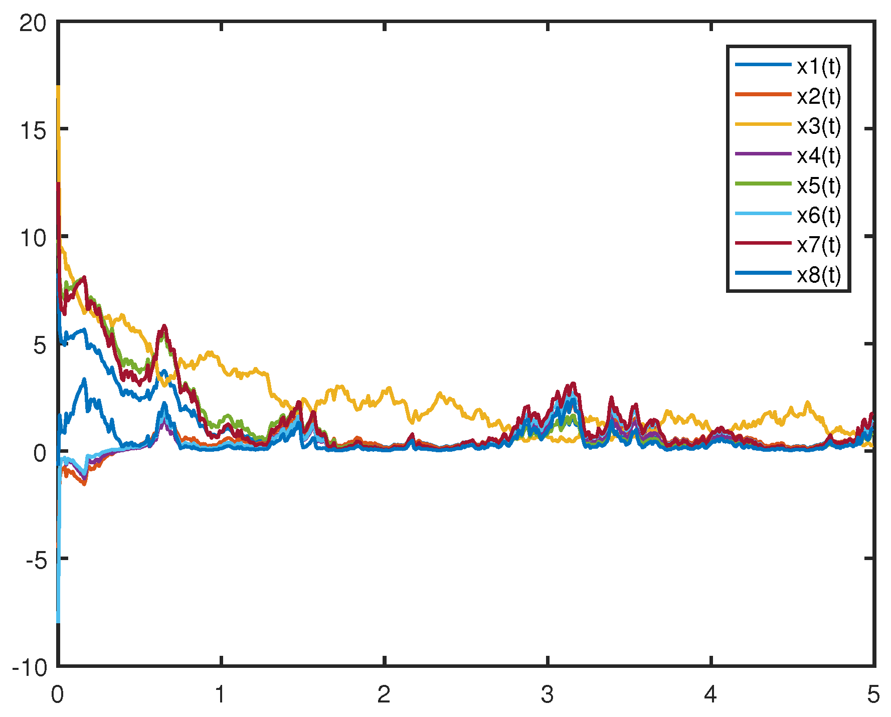
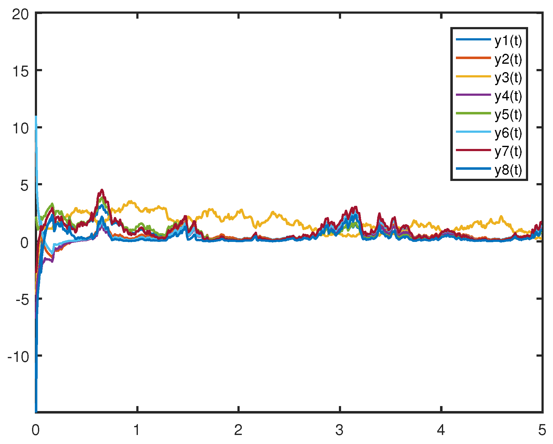
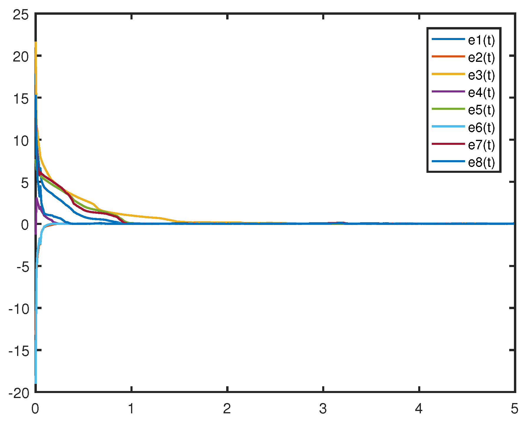
The trajectories of the drive system (24) and response system (25) are shown in Figure 1 and Figure 2, respectively. Figure 3 shows that the error system (26) in the absence of control does not tend to zero, which implies that drive system (24) and response system (25) can not achieve synchronization without control. Obviously, the drive system (24) and the response system (25) are gradually synchronized under the action of the feedback controller, because the trajectories of error system (26) with control in Figure 4 gradually drops to zero. The validity of Theorem 1 is verified.

5. Conclusions

In this paper, we investigate the synchronization problem of FSCNNs with discrete and infinite delays. By using a feedback controller, we obtain some pth-moment exponential synchronization criterion for the neural networks. Moreover, we provide a numerical simulation example to verify the effectiveness of our results. At present, the research on the synchronization of neural networks with delays is mainly focused on the network with finite delays, and there is not much research on the neural networks with infinite delays. Our paper provides some new results on infinite delay networks.

Through Theorem 1, we can limit the coefficient values of the controller so that the network achieves synchronization. However, the form of the decision conditions and the calculation of some values in Theorem 1, such as $\zeta$, are more complicated. On the basis of this study, perhaps we can try to use adaptive controller, fuzzy controller, state feedback controller, and other means to study the synchronization control of FSCNNs with infinite delays, so as to obtain a conclusion with a lower computational complexity. At the same time, we can also try to consider the topological structure of FSCNNs on the basis of the original research, so as to better optimize the control strategy and improve the synchronization control efficiency.

There are many interesting questions that deserve to be investigated for FSCNNs with infinite delays. The neural network in this paper is affected by continuous random perturbations (white noise). In fact, discontinuous random perturbations (Levy noise) should also be considered that can be used to describe the sudden external influences. Moreover, we obtain the asymptotic synchronization of FSCNNs with infinite delays, but it is not clear whether FSCNNs can achieve synchronization at a finite or fixed time.

References

1. Ayrulu, B.; Barshan, B. Neural networks for improved target differentiation and localization with sonar. Neural Netw. 2001, 14, 355–373. [Google Scholar] [CrossRef] [PubMed]
2. Han, Q.; Cao, R.; Liu, J.; Huang, J.J.; Yi, J.; Liu, C.; Weng, T.F. Analysis of associative memories based on cellular neural networks with value-varying templates. Int. J. Comput. Math. 2019, 96, 2024–2038. [Google Scholar] [CrossRef]
3. Li, C.; Xu, X.F.; Liu, M. The Stochastic fixed-time synchronization of delays neural networks driven by lévy noise. Syst. Control Lett. 2024, 190, 105839. [Google Scholar] [CrossRef]
4. Park, J.H. Synchronization of cellular neural networks of neutral type via dynamic feedback controller. Chaos Soliton Fract. 2009, 42, 1299–1304. [Google Scholar] [CrossRef]
5. Hou, L.L.; Ma, P.F.; Ma, X.; Sun, H.B. H exponential synchronization of switched cellular neural networks based on disturbance observer-based control. Int. J. Control Autom. Syst. 2024, 22, 1430–1441. [Google Scholar] [CrossRef]
6. Skrzypek, L.; You, Y.C. Feedback synchronization of FHN cellular neural networks. Discret. Contin. Dyn. Syst.-Ser. B 2021, 26, 6047–6056. [Google Scholar] [CrossRef]
7. Yang, T.; Yang, L.B.; Wu, C.W.; Chua, L.O. Fuzzy cellular neural networks: Applications. In Proceedings of the 1996 Fourth IEEE International Workshop on Cellular Neural Networks and their Applications Proceedings (CNNA-96), Seville, Spain, 24–26 June 1996; pp. 225–230. [Google Scholar]
8. Abdurahman, A.; Jiang, H.J.; Teng, Z.D. Finite-time synchronization for fuzzy cellular neural networks with time-varying delays. Fuzzy Sets Syst. 2016, 297, 96–111. [Google Scholar] [CrossRef]
9. Ma, W.Y.; Li, C.P.; Wu, Y.J. Synchronization of fractional fuzzy cellular neural networks with interactions. Chaos: Interdiscip. J. Nonlinear Sci. 2017, 27, 103106. [Google Scholar] [CrossRef]
10. Yu, J.; Hu, C.; Jiang, H.J.; Teng, Z.D. Exponential lag synchronization for delayed fuzzy cellular neural networks via periodically intermittent control. Math. Comput. Simul. 2012, 82, 895–908. [Google Scholar] [CrossRef]
11. Roska, T.; Chua, L.O. Cellular neural networks with nonlinear and delay-type template elements. In Proceedings of the IEEE International Workshop on Cellular Neural Networks and their Applications, Budapest, Hungary, 16–19 December 1990; pp. 12–25. [Google Scholar]
12. Ding, W.; Han, M.A. Synchronization of delayed fuzzy cellular neural networks based on adaptive control. Phys. Lett. 2008, 372, 4674–4681. [Google Scholar] [CrossRef]
13. Chen, L.; Zhao, H.Y. Stability analysis of stochastic fuzzy cellular neural networks with delays. Neurocomputing 2008, 72, 436–444. [Google Scholar] [CrossRef]
14. Zhang, Q.H.; Lin, F.B.; Wang, G.Y.; Long, Z.Q. Existence and stability of periodic solutions for stochastic fuzzy cellular neural networks with time-varying delay on time scales. Dyn. Syst. Appl. 2018, 27, 851–871. [Google Scholar]
15. Liu, Y.; Liu, M.; Xu, X.F. Adaptive control design for fixed-time synchronization of fuzzy stochastic cellular neural networks with discrete and distributed delay. Iran. J. Fuzzy Syst. 2021, 18, 13–28. [Google Scholar]
16. Xu, D.S.; Liu, Y.; Liu, M. Finite-time synchronization of multi-coupling stochastic fuzzy neural networks with mixed delays via feedback control. Fuzzy Sets Syst. 2021, 411, 85–104. [Google Scholar] [CrossRef]
17. Xu, D.S.; Wang, T.; Liu, M. Finite-time synchronization of fuzzy cellular neural networks with stochastic perturbations and mixed delays. Circuits Syst. Signal Process. 2021, 40, 3244–3265. [Google Scholar] [CrossRef]
18. Rakkiyappan, P.; Balasubramaniam, R. Global asymptotic stability of stochastic recurrent neural networks with multiple discrete delays and unbounded distributed delays. Appl. Math. Comput. 2008, 204, 680–686. [Google Scholar]
19. Wei, Z.; Xu, D.Y. Global exponential stability of fuzzy cellular neural networks with impulses and infinite delays. J. Math. Res. Expo. 2008, 28, 1–10. [Google Scholar]
20. Li, W.X.; Pang, L.S.; Su, H.; Wang, K. Global stability for discrete cohen–grossberg neural networks with finite and infinite delays. Appl. Math. Lett. 2012, 25, 2246–2251. [Google Scholar] [CrossRef]
21. Jiang, H.J.; Teng, Z.D. Boundedness, periodic solutions and global stability for cellular neural networks with variable coefficients and infinite delays. Neurocomputing 2009, 72, 2455–2463. [Google Scholar] [CrossRef]
22. Zhang, H.; Zeng, Z.G. Synchronization of recurrent neural networks with unbounded delays and time-varying coefficients via generalized differential inequalities. Neural Netw. 2021, 143, 161–170. [Google Scholar] [CrossRef]
23. He, P.; Li, H.; Luo, X.C.; Xing, M.L. Exponential synchronisation of linearly coupled reaction-diffusion neural networks with discrete and infinite distributed delays. Int. J. Syst. Sci. 2020, 51, 1174–1187. [Google Scholar] [CrossRef]
24. Li, X.; Fu, X. Stability analysis of stochastic functional differential equations with infinite delay and its application to recurrent neural networks. J. Comput. Appl. Math. 2010, 234, 407–417. [Google Scholar] [CrossRef]
25. Wang, X.B.; Wu, X.F.; Nie, Z.; Yan, Z.X. The pth moment exponential synchronization of drive-response memristor neural networks subject to stochastic perturbations. Complexity 2023, 2023, 1335184. [Google Scholar] [CrossRef]
26. Zhu, Q.X.; Cao, D.J. pth moment exponential synchronization for stochastic delayed cohen–grossberg neural networks with markovian switching. Nonlinear Dyn. 2011, 67, 829–845. [Google Scholar] [CrossRef]
27. Luo, J.W. Stability of stochastic partial differential equations with infinite delays. J. Comput. Appl. Math. 2008, 222, 364–371. [Google Scholar] [CrossRef]
28. Mao, X.R. Stochastic Differential Equations and Applications; Horwood: Chichester, UK, 1997. [Google Scholar]
29. Beckenbach, E.; Bellman, R. Inequalities; Springer: New York, NY, USA, 1961. [Google Scholar]
Figure 1. Drive system’s trajectories.
Axioms 14 00142 g001
Figure 2. Response system’s trajectories under controller.
Axioms 14 00142 g002
Figure 3. Error system’s trajectories without controller.
Axioms 14 00142 g003
Figure 4. Error system’s trajectories under controller action.
Axioms 14 00142 g004