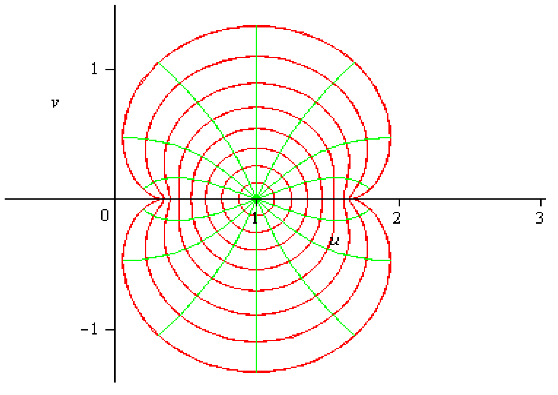
On Certain Analytic Functions Associated with Nephroid Function

Abstract

The normalized analytic function ${\Phi }_N\left(z\right)=1+z-{\displaystyle \frac{z^3}{3}}$, which connects the open unit disk onto a bounded domain within the right half of a nephroid-shaped region, is associated with the bounded turning of functions denoted by $R_n$. It calculates the sharp coefficient inequalities, which include the upper bound of the third Hankel determinant and Logarithmic coefficients related to the functions of the ${\Phi }_N\left(z\right)$ class. This research mainly focuses on identifying solutions to specific coefficient-related problems for analytic functions within the domain of nephroid functions.

1. Introduction and Definitions

Let A represent the class of function f defined by

$$f\left(z\right)=z+\sum _{n=2}^{\infty }{b}_n{z}^n(z\in E),$$

(1)

where these functions are analytic in the unit disk $E=\left\{z\in \mathbb{C}:\left|z\right|<1\right\}$. Let S represent a subclass of A that contains the univalent functions in E. For two functions, f and g, belonging to the set A, the function f is said to be subordinate to the function g, denoted as $f\prec g$, if an analytic function w satisfying $w\left(0\right)=0$ and $\left|w\right(z\left)\right|<1$ for all $z\in E$ exists, such that:

$$f\left(z\right)=g\left(w\right(z\left)\right).$$

The class of functions with bounded turning, introduced by the Zaprawa subclass [1], can be defined in the following way

$$R=\left\{f\in S:f^{\prime }\left(z\right)\prec \Phi \left(z\right)\right\},$$

where $\Phi$ is the analytic function that satisfies $Re(\Phi (z\left)\right)>0$ for all $z\in E$. We study the analytic function ${\Phi }_N\left(z\right)$ = $1+z-{\displaystyle \frac{z^3}{3}}$, which maps the domain E into the nephroid-shaped region. The nephroid curve is an important test case for studying the behavior of functions under geometric transformations in the complex plane. It helps researchers analyze how analytic functions map the unit disk to nephroid-shaped regions, allowing for the exploration of concepts such as starlikeness, convexity, and other geometric properties. This region is a nephroid shape symmetric to the real axis, as shown in Figure 1 below.

Using the above-mentioned function ${\Phi }_n$, we introduce the following class

$$\begin{array}{ccc}\hfill R_n& =& \left\{f\in S:f^{\prime }\left(z\right)\prec {\Phi }_N\left(z\right)\right\},\hfill \end{array}$$

for all $z\in E$.

The aim is to find the sharp bound for $\left|H_{3,1}\left(f\right)\right|$ and $\left|b_3{b}_5-b_4^2\right|$ for the class $R_n$.

For $n\ge 0$ and $q\ge 1$, Noonan and Thomas [2] determined the $q^{th}$ Hankel determinant of $f\in A$ of the form (1) in 1976.

$$H_{q,n}\left(f\right)=\left|\begin{array}{cccc}{b}_n\hfill & b_{n+1}\hfill & \cdots \hfill & b_{n+q-1}\hfill \\ b_{n+1}\hfill & b_{n+2}\hfill & \cdots \hfill & b_{n+q}\hfill \\ ⋮\hfill & ⋮\hfill & ⋮\hfill & ⋮\hfill \\ b_{n+q-1}\hfill & b_{n+q}\hfill & \cdots \hfill & b_{n+2q-2}\hfill \end{array}\right|.$$

The estimation of $|H_{2,2}\left(f\right)|$ has been the main focus of research on the Hankel determinant. Selvaraj and Kumar’s [3] proved $|H_{2,2}\left(f\right)|$$\le 1$ for the class C of convex functions. More results may be obtained from [4,5,6,7].

Many authors have explored these Hankel determinants for various subclasses of analytic and univalent functions. Sharp bounds for $|H_{3,1}\left(f\right)|$ were recently obtained utilizing a result from [8]; for more in depth studies on Hankel determinants, see [9,10,11,12,13,14].

$$H_{2,1}\left(f\right)=\left|\begin{array}{cc}\hfill b_1& b_2\\ \hfill b_2& b_3\end{array}\right|=b_3-b_2^2,$$

and

$$H_{2,2}\left(f\right)=\left|\begin{array}{cc}\hfill b_2& b_3\\ \hfill b_3& b_4\end{array}\right|=b_2{b}_4-b_3^2.$$

The determinant of Hankel $H_{2,1}\left(f\right)=b_3-b_2^2$.

In the current research, we study the Hankel determinant, represented by $H_{3,1}\left(f\right)$, for the cases $q=3$ and $n=1$.

$$H_{3,1}\left(f\right)=\left|\begin{array}{ccc}\hfill b_1& b_2& b_3\hfill \\ \hfill b_2& b_3& b_4\hfill \\ \hfill b_3& b_4& b_5\hfill \end{array}\right|.$$

When $b_1=1$ for $f\in A$, we obtain

$$H_{3,1}\left(f\right)=2b_2{b}_3{b}_4-b_3^3-b_4^2+b_5{b}_3-b_5{b}_2^2.$$

(2)

For the whole class $S\subset A$ of univalent functions, as well as for its subclasses, determining the growth of the Hankel determinant $H_{q,n}\left(f\right)$ depending on q and n is a fascinating problem to study. For class S, Pommerenke obtained some significant results [15]. The growth problem can be resolved to an estimate of the Hankel determinant for the suggested subclasses of A for fixed values of q and n. Srivastava et al. [16] discovered the same bound of Hankel and Toeplitz determinants for q-starlike functions connected to the generalized conic domain, while Arif et al. [17] determined the bound of the third Hankel determinant for functions associated with the sine function. Murugusundaramoorthy and Bulboacă [18] found the upper bound of Hankel determinants for certain analytic functions connected with the shell-shaped region. Khan et al. [19] determined the bound of third-order Hankel determinants for logarithmic coefficients of starlike functions connected with the sine function; Riaz et al. [20,21,22] studied the Hankel determinants for starlike and convex functions associated with the sigmoid function, lune, and cardioid domain; and Raza et al. [23] recently studied Hankel determinants for starlike functions connected with the symmetric Booth Lemniscate in 2022.

The logarithmic coefficients of $f\in S$, represented by ${\gamma }_n={\gamma }_n\left(f\right)$, are defined by the series expansion as follows:

$$log\left({\displaystyle \frac{f\left(z\right)}{z}}\right)=2\sum _{n=1}^{\infty }{\gamma }_n{z}^n.$$

The third logarithmic coefficient in certain subclasses of close-to-convex functions was studied by Cho et al. [24], while Ali et al. [25] studied the logarithmic coefficients of specific close-to-convex functions. For a function f given by (1), the logarithmic coefficients are as follows:

$${\gamma }_1={\displaystyle \frac{1}{2}}{b}_2,$$

(3)

$${\gamma }_2={\displaystyle \frac{1}{2}}\left(b_3-{\displaystyle \frac{1}{2}}{b}_2^2\right),$$

(4)

$${\gamma }_3={\displaystyle \frac{1}{2}}\left(b_4-b_2{b}_3+{\displaystyle \frac{1}{3}}{b}_2^2\right),$$

(5)

$${\gamma }_4={\displaystyle \frac{1}{2}}\left(b_5-b_2{b}_4+b_2^2{b}_3-{\displaystyle \frac{1}{2}}{b}_3^2-{\displaystyle \frac{1}{4}}{b}_2^4\right),$$

(6)

$${\gamma }_5={\displaystyle \frac{1}{2}}\left(b_6-b_2{b}_5-b_3{b}_4+b_2{b}_3^2+b_2^2{b}_4-b_2^3{b}_3+{\displaystyle \frac{1}{5}}{b}_2^5\right).$$

(7)

Based on all of the above ideas, we propose studying the Hankel determinant, where its entries are derived from the logarithmic coefficients of $f\in S$.

$$H_{q,n}\left(f\right)=\left|\begin{array}{cccc}{\gamma }_n& {\gamma }_{n+1}& \cdots & {\gamma }_{n+q-1}\\ {\gamma }_{n+1}& {\gamma }_{n+2}& \cdots & {\gamma }_{n+q}\\ ⋮& ⋮& \cdots & ⋮\\ {\gamma }_{n+q-1}& {\gamma }_{n+q}& \cdots & {\gamma }_{n+2q-2}\end{array}\right|.$$

From the above, it is easy to conclude that

$$H_{2,1}\left(f\right)={\gamma }_1{\gamma }_3-{\gamma }_2^2,$$

(8)

$$H_{2,2}\left(f\right)={\gamma }_2{\gamma }_4-{\gamma }_3^2.$$

(9)

The main aim of this article is to determine upper bounds for $H_{3,1}\left(f\right)$ for the class of nephroid functions.

Definition 1.

Let P denote the set of all functions p that are analytic in E and satisfy the condition $Re$$\left(p\right(z\left)\right)\ge 0$. These functions have the following series representation.

$$p\left(z\right)=1+\sum _{n=1}^{\infty }{c}_n{z}^n,z\in E.$$

(10)

2. A Set of Lemmas

Lemma 1.

If the series representation of the function $p\in P$ is as defined in (10), then

$$\left|c_{n+k}-\lambda c_n{c}_k\right|\le 2max\left\{1,\left|2\lambda -1\right|\right\}=\left\{\begin{array}{c}2\mathit{for}0\le \lambda \le 1;\hfill \\ 2\left|2\lambda -1\right|\mathit{otherwise}.\hfill \end{array}\right.$$

(11)

and

$$\left|c_n\right|\le 2\mathit{for}n\ge 1.$$

(12)

The proofs for two sharp inequalities (11) and (12) and can be obtained [26,27], respectively.

Lemma 2

([8]). If the series representation of the function $p\in P$ is as defined in (10) and if $B\in \left[0,1\right]$ with $B(2B-1)\le D\le B$, then

$$\left|c_3-2B{c}_1{c}_2+D{c}_1^3\right|\le 2.$$

(13)

Lemma 3.

If the series representation of the function $p\in P$ is as defined in (10), then x,$\delta ,\rho \in \overline{E}=\left\{z\in C:\left|z\right|\le 1\right\}$, we obtain

$$\begin{array}{cc}\hfill 2c_2& =\left(mx+c^2\right),\hfill \end{array}$$

(14)

$$\begin{array}{cc}\hfill 4c_3& =\left\{-m{x}^2{c+2mxc+2m(1-|x|}^2)\delta +c^3\right\},\hfill \end{array}$$

(15)

$$\begin{array}{cc}\hfill 8c_4& =\left[\begin{array}{c}\left(4x+\left(x^2-3x+3\right)c^2\right)mx-4m\left(1-{\left|x\right|}^2\right)\\ {-\rho (1-|\delta |}^2)+\left(x-1\right)\delta c+{\delta }^2\overline{x}+c^4\end{array}\right].\hfill \end{array}$$

(16)

where $m=(4-c^2)$, we can use the formula for $c_2$ within [26]. Libera and Zlotkiewicz [28] are recognized with the formula for $c_3$, while [29] for the formula of $c_4$.

Lemma 4

([30]). If the series representation of the function $p\in P$ is as defined in (10) and if $\eta ,a,\alpha$ and β satisfies the inequality conditions $0<\alpha <1$, $0<a<1$, and

$$8\left({(\alpha (b+\alpha )-\beta )}^2+{(\alpha \beta -2\eta )}^2\right)\left(1-b\right)b+\alpha {(\beta -2b\alpha )}^2(1-\alpha )\le 4b{\alpha }^2{(1-\alpha )}^2(1-b),$$

then,

$$\left|\eta c_1^4+b{c}_2^2+2\alpha c_1{c}_3-{\displaystyle \frac{3}{2}}\beta c_1^2{c}_2-c_4\right|\le 2.$$

(17)

3. Third Hankel Determinant for the Class $R_n$

In this section, we explore the sharp bound of the third-order Hankel determinant for $f\in R_n$.

Theorem 1.

If the series representation of the function $f\in R_n$ as given in (1), then

$$\left|H_{3,1}\left(f\right)\right|\le {\displaystyle \frac{1}{144}}.$$

The bound is sharp, and its sharpness can be attained from

$$f\left(z\right)=\underset{0}{\overset{z}{\int }}\left(1+\left(t-{\displaystyle \frac{t^3}{3}}\right)\right)dt=z+{\displaystyle \frac{1}{2}}{z}^2-{\displaystyle \frac{1}{12}}{z}^4+..{.}_{.}$$

Proof. 

Let $f\in R_n$. Then,

$$f^{\prime }\left(z\right)\prec 1+z-{\displaystyle \frac{z^3}{3}}.$$

(18)

If $p\in P$, then

$$p\left(z\right)={\displaystyle \frac{1+w\left(z\right)}{1-w\left(z\right)}}=1+c_{1}z+c_2{z}^2+c_{3}z+\cdots$$

Using (18), we obtain

$$\begin{array}{ccc}\hfill f^{\prime }\left(z\right)& =& 1+{\displaystyle \frac{1}{2}}{c}_{1}z+({\displaystyle \frac{1}{2}}{c}_2-{\displaystyle \frac{1}{4}}{c}_1^2)z^2+({\displaystyle \frac{1}{2}}{c}_3-{\displaystyle \frac{1}{2}}{c}_{1}c+{\displaystyle \frac{1}{12}}{c}_1^3)z^3\hfill \\ & & +\left({\displaystyle \frac{1}{2}}{c}_1{c}_3+{\displaystyle \frac{1}{4}}{c}_1^2{c}_2+{\displaystyle \frac{1}{2}}{c}_4-{\displaystyle \frac{1}{4}}{c}_2^2\right)z^4+\cdots .\hfill \end{array}$$

(19)

Considering that the series is defined in (1), it implies that

$$f^{\prime }\left(z\right)=1+2b_{2}z+3b_3{z}^2+4b_4{z}^3+\cdots .$$

(20)

Comparing (20) and (19), we have

$$\begin{array}{cc}\hfill b_2& ={\displaystyle \frac{1}{4}}{c}_1,\hfill \end{array}$$

(21)

$$\begin{array}{cc}\hfill b_3& ={\displaystyle \frac{1}{6}}{c}_2-{\displaystyle \frac{1}{12}}{c}^2,\hfill \end{array}$$

(22)

$$\begin{array}{cc}\hfill b_4& ={\displaystyle \frac{1}{8}}{c}_3-{\displaystyle \frac{1}{8}}{c}_{1}c+{\displaystyle \frac{1}{48}}{c}_1^3,\hfill \end{array}$$

(23)

$$\begin{array}{cc}\hfill b_5& =-{\displaystyle \frac{1}{10}}{c}_1{c}_3+{\displaystyle \frac{1}{20}}{c}_1^2{c}_2+{\displaystyle \frac{1}{10}}{c}_4-{\displaystyle \frac{1}{20}}{c}_2^2.\hfill \end{array}$$

(24)

Substituting the expressions (21)–(24) into (2) and setting $c_1=c$, we have

$$H_{3,1}\left(f\right)={\displaystyle \frac{1}{L}}\left(\begin{array}{c}936c{c}_2{c}_3-25c^6-448c_2^3+780c^2{c}_2^2-312c_2{c}^4-864c^3{c}_3-360c_2{c}^3\\ -540c_3^2+576c_2{c}_4-540c^4-504c^2{c}_4+1080c^2{c}_3+360c^5\end{array}\right),$$

(25)

where $L=34560$. Now, letting $c_1=c$ and $m=(4-c^2)$, we obtain

$$\begin{array}{cc}\hfill c_2& ={\displaystyle \frac{1}{2}}\left(mx+c^2\right),\hfill \\ \hfill c_3& ={\displaystyle \frac{1}{4}}\left\{-m{x}^2{c+2mxc+2m(1-|x|}^2)\delta +c^3\right\},\hfill \\ \hfill and\\ \hfill c_4& ={\displaystyle \frac{1}{8}}\left[\begin{array}{c}\left(4x+\left(x^2-3x+3\right)c^2\right)mx-4m\left(1-{\left|x\right|}^2\right)\\ {-\rho (1-|\delta |}^2)+\left(x-1\right)\delta c+{\delta }^2\overline{x}+c^4\end{array}\right].\hfill \end{array}$$

Then, from (25), we have

$$H_{3,1}\left(f\right)={\displaystyle \frac{1}{L}}\left\{\begin{array}{c}{\displaystyle \frac{-11}{4}}{c}^6-420c^4+9x\delta c^3+20c^3+135{(4-c^2)}^2{x}^{2}c(1-{\left|x\right|}^2)\delta \\ -36{(4-c^2)}^{2}xc(1-{\left|x\right|}^2)\delta +88(4-c^2)x^3-9\delta c^3+36\delta c^2\\ -9\rho c^2+36c\rho +111c^5+234c^2{(4-c^2)}^2{x}^2+{\displaystyle \frac{45}{2}}(4-c^2)x^2{c}^4\\ -195(4-c^2)x{c}^2-36(4-c^2)c^3{x}^3+135{(4-c^2)}^2{x}^3{c}^2+36{\delta }^2{x}^2(4-c^2)\\ -144{(4-c^2)}^2(1-{\left|x\right|}^2)x-36\delta c^{2}x-45(4-c^2)x^2{c}^3\\ +144c(4-c^2)(1-{\left|x\right|}^2)+9{\delta }^{2}x{c}^2+138(4-c^2)x{c}^3+75(4-c^2)x^2{c}^2\\ -48(4-c^2)x^{2}c-135(4-c^2){(1-{\left|x\right|}^2)}^2{\delta }^2-225(4-c^2)x^3{c}^2\\ -36c{\delta }^{2}x-36\rho (4-c^2)x-36c^2(4-c^2)(1-{\left|x\right|}^2)+9(4-c^2)c^4{x}^3\\ +87(4-c^2)x{c}^4+36\delta c{x}^2(4-c^2)-99c^3(4-c^2)(1-{\left|x\right|}^2)\delta \\ +306c^2(4-c^2)(1-{\left|x\right|}^2)\delta -36xc(4-c^2)\delta +{\displaystyle \frac{9}{4}}(4-c^2)x^4{c}^2\end{array}\right\}.$$

Since $m=(4-c^2)$, it follows that

$$H_{3,1}\left(f\right)={\displaystyle \frac{1}{L}}\left(m_0(c,x)+m_1(c,x)\delta +m_2(c,x){\delta }^2+\Pi (c,x,\delta )\rho \right),$$

where $\rho$, x, $\delta$∈$\overline{E}$, and

$$\begin{array}{cc}\hfill m_0(c,x)& =(4-c^2)\left[\begin{array}{c}{\displaystyle \frac{9}{4}}{c}^2+88x^3+{\displaystyle \frac{45}{2}}{x}^2{c}^4-195x{c}^2-36c^3{x}^3-45x^2{c}^3\\ +138x{c}^3-48x^{2}c+75x^2{c}^2-225x^3{c}^2+9c^4{x}^3+87x{c}^4\\ +(4-c^2)\left(234c^2{x}^2+135x^3{c}^2\right)\end{array}\right]\hfill \\ \hfill & {\displaystyle \frac{-11}{4}}{c}^6+111c^5-420c^4+20c^3,\hfill \end{array}$$

$$\begin{array}{cc}\hfill m_1(c,x)& =(4-c^2)\left[\begin{array}{c}135(4-c^2)x^{2}c(1-{\left|x\right|}^2)-36(4-c^2)xc(1-{\left|x\right|}^2)\\ -99c^3(1-{\left|x\right|}^2)+306c^2(1-{\left|x\right|}^2)-36xc+36c{x}^2\end{array}\right]\hfill \\ \hfill & +9x{c}^3-9c^3+36c^2-36c^{2}x,\hfill \end{array}$$

$$\begin{array}{cc}\hfill m_2(c,x)& =(4-c^2)\left[36{\delta }^2{x}^2-135{(1-{\left|x\right|}^2)}^2\right]\hfill \\ \hfill & +9x{c}^2-36cx,\hfill \end{array}$$

and

$$\begin{array}{cc}\hfill \Pi (c,x,\delta )& =9\left[-c^2+4c-4(4-c^2)x\right].\hfill \end{array}$$

Taking $\left|\rho \right|\le 1$ and replacing $\left|\delta \right|$ by y and $\left|x\right|$ by x, one obtains

$$|H_{3,1}\left(f\right)|\le {\displaystyle \frac{1}{L}}\left(\left|\right(m_0(c,x)|+|m_1(c,x)|y+|m_2(c,x)|y^2+|\Pi (c,x,\delta )|\right)\le {\displaystyle \frac{1}{L}}\left(f(c,x,y)\right),$$

(26)

where

$$f(c,x,y)=\left(n_0(c,x)+n_1(c,x)y+n_2(c,x)y^2+n_3(c,x)(1-y^2)\right),$$

(27)

with

$$\begin{array}{cc}\hfill n_0(c,x)& =(4-c^2)\left[\begin{array}{c}{\displaystyle \frac{9}{4}}{c}^2+88x^3+{\displaystyle \frac{45}{2}}{x}^2{c}^4+195x{c}^2+36c^3{x}^3+45x^2{c}^3\\ +138x{c}^3+48x^{2}c+75x^2{c}^2+225x^3{c}^2+9c^4{x}^3+87x{c}^4\\ +(4-c^2)\left(234c^2{x}^2+135x^3{c}^2\right)\end{array}\right]\hfill \\ \hfill & +{\displaystyle \frac{11}{4}}{c}^6+111c^5+420c^4+20c^3,\hfill \\ \hfill n_1(c,x)& =(4-c^2)\left[\begin{array}{c}135(4-c^2)x^{2}c(1-x^2)+36(4-c^2)xc(1-x^2)\\ +99c^3(1-x^2)+306c^2(1-x^2)+36xc+36c{x}^2\end{array}\right]y\hfill \\ \hfill & +9x{c}^{3}y+9c^{3}y+36c^{2}y+36c^{2}xy,\hfill \\ \hfill n_2(c,x)& =(4-c^2)\left[{36}^2{x}^2+135{(1-x^2)}^2\right]y^2\hfill \\ \hfill & +9x{c}^2{y}^2+36cx{y}^2,\hfill \\ \hfill and\\ \hfill n_3(c,x)& =9\left[c^2+4c+4(4-c^2)x\right]\left(1-y^2\right).\hfill \end{array}$$

Then, the partial derivative of the function (27) by ‘y’, is given by

$$\begin{array}{ccc}\hfill {\displaystyle \frac{\partial f}{\partial y}}& =& 36c(4-c^2)x+36(4-c^2)x^{2}c+99c^3(4-c^2)(1-x^2)\hfill \\ & & +306c^2(4-c^2)(1-x^2)+72cyx+18y{c}^{2}x+36c^{2}x\hfill \\ & & +270(4-c^2){(1-x^2)}^{2}y+9c^{3}x+72y{x}^2(4-c^2)\hfill \\ & & +504c{(4-c^2)}^{2}x(1-x^2)+135{(4-c^2)}^2{x}^{2}c(1-x^2)\hfill \\ & & +9c^3+36c^2.\hfill \end{array}$$

Taking ${\displaystyle \frac{\partial f}{\partial y}}=0,$ we have

$$y={\displaystyle \frac{-c\left(\begin{array}{c}-45c^2+34c^3+11c^4+451c^{2}x-4cx\\ -912x+168c^2{x}^2+136x^{2}c-26c^4{x}^2\\ -34x^2{c}^3+240x^4-120c^2{x}^4+15x^4{c}^4\\ +896x^3-448c^2{x}^3-56c^{4}x+56c^4{x}^3\\ -256x^2-140c.\end{array}\right)}{2(-c^{2}x-60+104x^2-60x^4+15c^2-26c^2{x}^2+15c^2{x}^4-4cx)}}:=y_1.$$

For $y_1$ to belong to $\left(0,1\right)$, it is possible only if

$$\begin{array}{ccc}& & \left(\begin{array}{c}45c^3-34c^4-11c^5-451c^{3}x+4c^{2}x\\ +912cx-168c^3{x}^2-136x^2{c}^2+26c^5{x}^2\\ +34x^2{c}^4-240x^{4}c+120c^3{x}^4-15x^4{c}^5\\ -896x^{3}c+448c^3{x}^3+56c^{5}x-56c^5{x}^3\\ +256x^{2}c-140c^2\end{array}\right)\hfill \\ & <& 2(-c^{2}x-60+104x^2-60x^4+15c^2-26c^2{x}^2+15c^2{x}^4-4cx),\hfill \end{array}$$

(28)

and

$$c^2>{\displaystyle \frac{\begin{array}{c}-26c^5{x}^2+15x^4{c}^5-56c^{5}x+56c^5{x}^3\\ +11c^5+34c^4-34c^4{x}^2+451c^{3}x\\ -448c^3{x}^3+168x^2{c}^3-120x^4{c}^3-45c^3\\ +896c{x}^3-912cx+240x^{4}c-256x^{2}c\end{array}}{140-136x^2+4x}}.$$

(29)

Suppose,

$$g\left(x\right)={\displaystyle \frac{\begin{array}{c}-26c^5{x}^2+15x^4{c}^5-56c^{5}x+56c^5{x}^3\\ +11c^5+34c^4-34c^4{x}^2+451c^{3}x\\ -448c^3{x}^3+168x^2{c}^3-120x^4{c}^3-45c^3\\ +896c{x}^3-912cx+240x^{4}c-256x^{2}c\end{array}}{140-136x^2+4x}}.$$

This gives

$$\begin{array}{c}{g}^{\prime }\left(x\right)=31920c+45920cx-1020c^5{x}^3-16320c{x}^3+2896x^{2}c+181c^5{x}^2\hfill \\ -1448c^3{x}^2-22960c^{3}x+2870c^{5}x+45920cx-31920c\hfill \\ -34c^4+15830c^3-1971c^5\hfill \\ =h\left(x\right).\hfill \end{array}$$

Since $g^{\prime }\left(x\right)<0$ for $x\in (0,1),$ as can be seen from the graph of $h\left(x\right)$ in Figure 2.

It follows that $g\left(x\right)$ decreases in $(0,1)$. Therefore, $c^2>{\displaystyle \frac{6c^3-32c}{8}}$, and calculation shows that f has no critical points in $(0,2)\times (0,1)\times (0,1)$. As a result, (28) does not hold for all $x\in (0,1)$. To determine the value of c, we consider the function to be greater than zero. In the original function, we need to substitute the minimum value of the original function. Proper calculation of time is possible. If you have the interval $x\in (0,1)$ or if you restrict the interval to a certain number, substitute that number into $g\left(x\right)$. The value of $c^2$ obtained from both the original interval $x\in (0,1)$ and the restricted interval will be the same. In that case, the inequality will still hold, and a critical point will exist. There is no such number that, when restricting the interval, would cause the inequality to be unsatisfied.

Next, we will explore the maxima of $f(c,x,y)$ within the interiors of all six faces of $\Delta .$ Using $c=0$ in (27), we obtain

$$p_1(x,y)=f(0,x,y)=2448x-1504x^3-936y^2{x}^2+540y^2+540y^2{x}^4.$$

Consequently, $(x,y)$ belongs to $(0,1)\times (0,1)$, we have not found any maxima for $f(0,x,y)$. If we take $c=2$ in (27), we obtain

$$f(2,x,y)=10716+108y^{2}x+216yx+216y.$$

(30)

Putting $x=0$ in (27), we obtain

$$\begin{array}{cc}{p}_2(x,y)& =f(c,0,y)=405y{c}^3-99y{c}^5+1260y{c}^2-306y{c}^4+612c-124c^3+384c^4\\ & +153c^2+111c^5+{\displaystyle \frac{11}{4}}{c}^6+540y^2-135y^2{c}^2.\end{array}$$

By solving ${\displaystyle \frac{\partial p_2}{\partial y}}=0$ and ${\displaystyle \frac{\partial p_2}{\partial c}}=0,$ the critical point if ${\displaystyle \frac{\partial p_2}{\partial y}}=0,$ we have

$$y={\displaystyle \frac{-c^2(-45c+11c^3-140+34c^2)}{30(c^2-4)}}:=y_0.$$

(31)

Further, ${\displaystyle \frac{\partial p_2}{\partial c}}=0$, gives

$$1215y{c}^2-495y{c}^4+2520yc-1224y{c}^3+612-372c^2+1536c^3+306c+555c^4+{\displaystyle \frac{33}{2}}{c}^5-270y^{2}c=0.$$

By inserting (31) into the above equation, we have

$$\begin{array}{cc}\hfill & 97920-38898c^7-5601c^9-80892c^8+1452c^{11}+48960c-249120c^3\hfill \\ & -108480c^2-253320c^4+211440c^5+266460c^6+7854c^{10}=0.\hfill \end{array}$$

Now, solving for $c\in (0,2)$, we obtain $c\simeq 1.693$. Therefore, no optimal solution exists for $f(c,x,y)$ in $(0,2)\times (0,1)$. When $x=1$ in (27), we obtain

$$\begin{array}{cc}\hfill p_3(c,y)& =f(c,1,y)=944+996c+7936c^2+2864c^3-660c^5+{\displaystyle \frac{5}{4}}{c}^6+72y{c}^2\hfill \\ \hfill & -{\displaystyle \frac{6459}{4}}{c}^4-54y{c}^3-27y^2{c}^2+36c{y}^2+144y^2+288yc.\hfill \end{array}$$

(32)

If $p_3$ has no critical point, then ${\displaystyle \frac{\partial p_3}{\partial c}}=0$. Considering $y=0$ in (27), we have

$$\begin{array}{cc}\hfill p_4(c,x)=f(c,x,0)& =384x^{2}c+279x^4{c}^2+1896c^{3}x+2448x+612c\hfill \\ \hfill & -1504x^3-408c^{2}x+153c^2-124c^3+111c^5+{\displaystyle \frac{11}{4}}{c}^6\hfill \\ \hfill & +384c^4+948x^2{c}^3-261c^5{x}^2-1605c^4{x}^2+144c^3{x}^3\hfill \\ \hfill & -474c^{5}x-36c^5{x}^3+3900c^2{x}^2+4012c^2{x}^3+126c^6{x}^3\hfill \\ \hfill & +{\displaystyle \frac{315}{2}}{c}^6{x}^2-{\displaystyle \frac{279}{4}}{x}^4{c}^4-285c^{6}x+1089c^{4}x-1413c^4{x}^3.\hfill \end{array}$$

If we take

$${\displaystyle \frac{\partial p_4}{\partial c}}=0\mathrm{and}{\displaystyle \frac{\partial p_4}{\partial x}}=0,$$

The solution does not exist in $\left(0,2\right)\times \left(0,1\right)$.

Taking $y=1$ in (27), we obtain

$$\begin{array}{cc}\hfill p_5(c,x)& =f(c,x,1)=540+2688x^{2}c+144x^4{c}^2-2163c^{3}x+2448x\hfill \\ \hfill & +612c-1504x^3-363c^{2}x+1278c^2-936x^2+281c^3\hfill \\ \hfill & +12c^5+{\displaystyle \frac{11}{4}}{c}^6+78c^4+8244cx-564x^2{c}^3-27c^5{x}^2\hfill \\ \hfill & -1299c^4{x}^2-2160x^{4}c+1080x^4{c}^3-135x^4{c}^5-8064c{x}^3\hfill \\ \hfill & +4176c^3{x}^3+30c^{5}x-540c^5{x}^3+2910c^2{x}^2+4012c^2{x}^3\hfill \\ \hfill & +126c^6{x}^3+{\displaystyle \frac{315}{2}}{c}^6{x}^2-{\displaystyle \frac{279}{4}}{x}^4{c}^4-285c^{6}x+1089c^{4}x\hfill \\ \hfill & -1413c^4{x}^3+540x^4.\hfill \end{array}$$

If we take

$${\displaystyle \frac{\partial p_5}{\partial x}}=0\mathrm{and}{\displaystyle \frac{\partial p_5}{\partial c}}=0,$$

The solution does not exist in $\left(0,2\right)\times \left(0,1\right)$. Finally, we evaluate the maximum $f(c,x,y)$ close to $\Delta$ at the 12 edges.

When we substitute $x=0$ and $y=0$ in (27), we have

$$p_6\left(c\right)=f(c,0,0)=612c+153c^2-124c^3+111c^5+{\displaystyle \frac{11}{4}}{c}^6+384c^4.$$

(33)

It can be observed that ${\displaystyle \frac{\partial p_6}{\partial c}}>0$ for $c\in [0,2]$, indicating that $p\left(c\right)$ is an increasing function on the interval $[0,2]$. Therefore, it reaches its maximum value at $c=2$.

$$f(c,0,0)=10716.$$

Put $x=0$, $y=1$ in (27), we obtain

$$p_7\left(c\right)=f(c,0,1)={\displaystyle \frac{11}{4}}{c}^6+281c^3+12c^5+540+78c^4+1278c^2+612c+540.$$

It can be observed that ${\displaystyle \frac{\partial p_7}{\partial c}}>0$ for $c\in [0,2]$, indicating that $p\left(c\right)$ is an increasing function on the interval $[0,2]$. Therefore, it reaches its maximum value at $c=2$.

$$f(c,0,1)\le 10932.$$

Put $c=0$, $x=0$ in (27), we obtain

$$p_8\left(y\right)=f(0,0,y)=540y^2.$$

Clearly, ${\displaystyle \frac{\partial p_8}{\partial c}}>0$ is obvious, while $p_8\left(y\right)$ increases for $\left[0,1\right]$, finding its maximum value at $y=1$, we obtain

$$f(0,0,y)\le 540.$$

Put $x=1$, $y=1$ and $y=0$ in (27), we obtain

$$p_9\left(c\right)=f(c,1,1)={\displaystyle \frac{5}{4}}{c}^6-660c^5+1320c+2810c^3-{\displaystyle \frac{6459}{4}}{c}^4+7981c^2+1088.$$

$$p_9\left(c\right)=f(c,1,0)={\displaystyle \frac{5}{4}}{c}^6-660c^5+996c+2864c^3-{\displaystyle \frac{6459}{4}}{c}^4+7936c^2+944.$$

$$andf(c,1,1)\ne f(c,1,0).$$

It can be observed that ${\displaystyle \frac{\partial p_9}{\partial c}}>0$ for $c\in [0,2]$, indicating that $p\left(c\right)$ is an decreasing function on the interval $[0,2]$. Therefore, it reaches its maximum value at $c=1.641$.

$$f(c,1,1)=p_9\left(c\right)\le 17624.39191,f(c,1,0)=p_9\left(c\right)\le 17066.15522.$$

Put $c=0$, $x=1$ in (27), we obtain

$$p_{10}\left(y\right)=f(0,1,y)=944+144y^2.$$

Put $c=2$, $x=0$, $x=1$ and $y=1$, $y=0$ in (27), we obtain

$$f(2,0,y)\ne f(2,1,y)\ne f(2,x,1)\ne f(2,x,0).$$

Put $c=0$, $y=0$ in (27), we obtain

$$p_{11}\left(x\right)=f(0,x,0)=2448x-1952x^3.$$

The maximum value of the function is $x=1.112$. That is,

$$f(0,x,0)\le 654.120460.$$

Put $c=0$, $y=1$ in (27), we obtain

$$p_{12}\left(x\right)=f(0,x,1)=540-936x^2+540x^4+2448x-1504x^3.$$

We observe ${\displaystyle \frac{\partial p_{12}}{\partial x}}>0$, so $p_{12}$ reaches its maximum value at $x=0$, so we have

$$f(0,x,1)\le 540.$$

By using (26), we obtain

$$H_{3,1}\left(f\right)\le {\displaystyle \frac{1}{L}}\le \left(f(c,x,y)\right)\le {\displaystyle \frac{1}{144}}.$$

Hence, achieving the required result. □

Theorem 2.

If the series representation of the function $f\in R_n$ as given in (1), then

$$|b_3{b}_5-b_4^2|\le {\displaystyle \frac{1}{144}}.$$

The following function preserves equality and gives the best possible result.

$$f\left(z\right)=\underset{0}{\overset{z}{\int }}\left(1+\left(t-{\displaystyle \frac{t^3}{3}}\right)\right)dt=z+{\displaystyle \frac{1}{2}}{z}^2-{\displaystyle \frac{1}{12}}{z}^4+\cdots .$$

Proof. 

Substituting (22)–(24) with $c_1=c$, we have

$$b_3{b}_5-b_4^2={\displaystyle \frac{1}{11520}}\left(\begin{array}{c}168c{c}_2{c}_3-36c^2{c}_2^2+192c_2{c}_4-96c_2^3+36c^3{c}_3\\ +12c^4{c}_2-96c^2{c}_4-5c^6-180c_3^2\end{array}\right).$$

(34)

By applying the resulting form of Equations (14)–(16), with $m=(4-c^2)$, we have

$$\begin{array}{cc}\hfill 168c{c}_2{c}_3& =-21m^2{x}^3{c}^2+42m^2{x}^2{c}^2+42c{m}^{2}x\delta (1-x^2)+63mx{c}^4-21c^4{x}^{2}m\hfill \\ \hfill & +42c^3\delta m(1-x^2)+21c^6,\hfill \\ \hfill 36c^2{c}_2^2& =-9m^2{x}^2{c}^2-18mx{c}^4-9c^6,\hfill \\ \hfill 192c_2{c}_4& =48m^2{x}^3+12m^2{c}^2{x}^4-36m^2{c}^2{x}^3+36x^2{m}^2{c}^2-48x{m}^2+48x^3{m}^2{-12xm\rho (1-|\delta |}^2)\hfill \\ \hfill & +12x^{2}m\delta c-12xm\delta c+12x^{2}m{\delta }^2+12xm{c}^4+48c^2{x}^{2}m+12c^4{x}^{3}m-36c^4{x}^{2}m\hfill \\ \hfill & +36c^{4}xm-48c^{2}m+48c^{2}m{x}^2-12c^2{\rho (1-|\delta |}^2)+12c^3\delta x-12c^3\delta +12c^2{\delta }^{2}x+12c^6,\hfill \\ \hfill 96c_2^3& =-12m^3{x}^3-36m^2{x}^2{c}^2-36mx{c}^4-12c^6,\hfill \\ \hfill 36c^3{c}_3& =-9x^2{c}^{4}m+18xm{c}^4+18c^3\delta m(1-x^2)+9c^6,\hfill \\ \hfill 12c^4{c}_2& =6mx{c}^4+6c^6,\hfill \\ \hfill 96c^2{c}_4& =-96m{x}^2{c}^2-12m{x}^3{c}^4+36m{x}^2{c}^4-36mx{c}^4+48m{c}^2{+12\rho (1-|\delta |}^2)c^2-12\delta x{c}^3\hfill \\ \hfill & +12\delta c^3-12x{c}^2{\delta }^2-12c^6,\hfill \\ \hfill and\\ \hfill 180c_3^2& ={\displaystyle \frac{45}{4}}{c}^6-{\displaystyle \frac{45}{2}}{x}^2{c}^{4}m+45x^{4}c{m}^2\delta +45\delta m{x}^2{c}^3-45xm{c}^4-{\displaystyle \frac{45}{4}}{x}^4{c}^2{m}^2-90xc\delta m^2\hfill \\ \hfill & -45x^3{c}^2{m}^2-45\delta c{x}^2{m}^2+90\delta c{x}^3{m}^2-45x{c}^2{m}^2-45m{\delta }^2+90m{\delta }^2{x}^2\hfill \\ \hfill & -45m\delta c^3-45m{\delta }^2{x}^4.\hfill \end{array}$$

By inserting the above expressions in (34), we have

$$b_3{b}_5-b_4^2={\displaystyle \frac{1}{L}}\left\{\begin{array}{c}-21m^2{x}^3{c}^2+42m^2{x}^2{c}^2+42\delta c{m}^{2}x(1-x^2)+21mx{c}^4-21m{x}^2{c}^4+42mx{c}^4+\\ 42\delta m{c}^3(1-x^2)+21c^6-9m{x}^2{c}^2-18mx{c}^4-9c^6+48m^2{x}^3+12m^2{x}^4{c}^2\\ -36m^2{c}^2{x}^3+36x^2{m}^2{c}^2-48x{m}^2+48m^2{x}^3{-12xm\rho (1-|\delta |}^2)+12x^{2}m\delta c\\ -12xm\delta c+12m{x}^2{\delta }^2+12xm{c}^4+48c^2{x}^{2}m+12x^3{c}^{4}m-36c^4{x}^{2}m+36c^{4}xm\\ -48c^{2}m+48c^{2}m{x}^2-12c^2{\rho (1-|\delta |}^2)+12c^3\delta x-12c^3\delta +12c^2{\delta }^{2}x+12c^6\\ -12m{x}^3-36m{x}^2{c}^2-36mx{c}^4-12c^6-9x^2{c}^{4}m+18x{c}^{4}m+18c^3\delta m(1-x^2)\\ -9c^6+6mx{c}^4+6c^6-96m{x}^2{c}^2-12m{x}^3{c}^4+36c^{4}m{x}^2-36mx{c}^4+48m{c}^2\\ {+12\rho (1-|\delta |}^2)c^2-12x\delta c^3+12c^3\delta -12c^2{\delta }^{2}x-12c^6-5c^6-{\displaystyle \frac{45}{4}}{c}^6+{\displaystyle \frac{45}{2}}{x}^2{c}^{4}m\\ +45x^{4}c{m}^2\delta +45x^{2}m\delta c^3-45xm{c}^4-{\displaystyle \frac{45}{4}}{x}^4{c}^2{m}^2-90xc{m}^2\delta -45x^3{c}^2{m}^2\\ +45x^{2}c{m}^2\delta +90x^{3}c{m}^2\delta -45x{c}^2{m}^2-45m^2{\delta }^2+12m{\delta }^2{x}^2-45m\delta c^3-45m{\delta }^2{x}^4\end{array}\right\}.$$

As $m=(4-c^2),$ it follows that

$$b_3{b}_5-b_4^2={\displaystyle \frac{1}{11520}}\left(b_0(c,x)+b_1(c,x)\delta +b_2(c,x){\delta }^2+b_3(c,x,\delta )\rho \right),$$

where $\delta ,\rho ,x\in \overline{E}$, and

$$\begin{array}{cc}\hfill b_0(c,x)& ={\displaystyle \frac{85}{4}}{c}^6+\left(\begin{array}{c}-{\displaystyle \frac{159}{2}}{c}^4{x}^2+33c^{4}x-48c^2-12x^3-36x{c}^4\\ -27x{c}^4-93x^2{c}^2+12x{c}^4+48c^2{x}^2+12c^4{x}^3\\ -48c^2-9x^2{c}^4+18x{c}^4-12x^3{c}^4+36c^4{x}^2\\ +(4-c^2)(-21x^3{c}^2+78x^2{c}^2-48x+96x^3\\ +{\displaystyle \frac{3}{4}}{c}^2{x}^4-81c^2{x}^3-45x{c}^2)\end{array}\right)(4-c^2),\hfill \\ \hfill b_1(c,x)& =\left(\begin{array}{c}60c^3(1-x^2)-12xc+12x^{2}c+45x^2{c}^3-45c^3\\ +(4-c^2)(45c{x}^4-45x^{2}c-90xc+42cx(1-x^2)+90x^{3}c)\end{array}\right)(4-c^2),\hfill \\ \hfill b_2(c,x)& =\left(-45+102x^2-45x^4\right)(4-c^2),\hfill \\ \hfill and\\ \hfill b_3(c,x)& ={-12(1-|\delta |}^2)(4-c^2)x.\hfill \end{array}$$

If we apply $\left|\rho \right|\le 1$ and then by substituting $\left|\delta \right|$ for y and $\left|x\right|$ by x, it can be concluded that

$$|b_3{b}_5-b_4^2|\le {\displaystyle \frac{1}{11520}}\left(|b_0(c,x)|+|b_1(c,x)|y+b_2(c,x)|y^2+\left|b_3(c,x,\delta )\right|\right)\le {\displaystyle \frac{1}{11520}}\left(f(c,x,y)\right),$$

(35)

where

$$f(c,x,y)=\left(h_0(c,x)+h_1(c,x)y+h_2(c,x)y^2+h_3(c,x)(1-y^2)\right),$$

(36)

with

$$\begin{array}{cc}\hfill h_0(c,x)& ={\displaystyle \frac{85}{4}}{c}^6+\left(\begin{array}{c}{\displaystyle \frac{159}{2}}{c}^4{x}^2+33c^{4}x+48c^2+12x^3+36x{c}^4\\ +27x{c}^4+93x^2{c}^2+12x{c}^4+48c^2{x}^2+12c^4{x}^3\\ +48c^2+9x^2{c}^4+18x{c}^4+12x^3{c}^4+36c^4{x}^2\\ +(4-c^2)(21x^3{c}^2+78x^2{c}^2+48x+96x^3\\ +{\displaystyle \frac{3}{4}}{c}^2{x}^4+81c^2{x}^3+45x{c}^2)\end{array}\right)(4-c^2),\hfill \\ \hfill h_1(c,x)& =\left(\begin{array}{c}60c^3(1-x^2)+12xc+12x^{2}c+45x^2{c}^3+45c^3\\ +(4-c^2)(45c{x}^4+45x^{2}c+90xc+42cx(1-x^2)+90x^{3}c)\end{array}\right)(4-c^2),\hfill \\ \hfill h_2(c,x)& =\left(45+102x^2+45x^4\right)(4-c^2),\hfill \\ \hfill and\\ \hfill h_3(c,x)& ={12(1-|\delta |}^2)(4-c^2)x.\hfill \end{array}$$

Differentiating (36) w.r.t ‘y’, using ${\displaystyle \frac{\partial f}{\partial y}}=0,$ we obtain

$${\displaystyle \frac{\partial f}{\partial y^{\prime }}}=\begin{array}{c}720x^{4}c+768x^{3}c+45c^5{x}^4+48c^{5}x+48c^5{x}^3+90y{c}^4\\ -360c^3{x}^4-384c^3{x}^3+2976x^{2}y+1440y{x}^4+180x^{2}y{c}^4\\ -720y{c}^2-1464x^{2}y{c}^2-720y{c}^2{x}^4+96xy-24xy{c}^2\\ +1440y+120c^3+768x^{2}c-372x^3{c}^2+90y{x}^4{c}^4\\ +816xc+45x^2{c}^5-396x{c}^3-30c^5.\end{array}$$

Taking ${\displaystyle \frac{\partial f}{\partial y}}=0,$ we have

$$y={\displaystyle \frac{-c\left(\begin{array}{c}-60x^4-64x^3+15x^4{c}^2+16c^2{x}^3+15x^2{c}^2\\ -68x-10c^2-64x^2+16x{c}^2\end{array}\right)}{2\left(-60x^4+15c^2-4x-60+30x^2{c}^2+15x^4{c}^2-124x^2\right)}}:=y_0.$$

$$\begin{array}{c}\hfill \begin{array}{c}(60x^4+64x^3-15x^4{c}^2-16c^2{x}^3-15x^2{c}^2+68x+10c^2+64x^2-16x{c}^2)>0,\end{array}\end{array}$$

(37)

and

$$c^2>{\displaystyle \frac{\begin{array}{c}-60x^4-64x^3-64x^2-68x\end{array}}{10-16x-15x^2-16x^3-15x^4}}.$$

(38)

Suppose,

$$g\left(x\right)={\displaystyle \frac{\begin{array}{c}-60x^4-64x^3-64x^2-68x\end{array}}{10-16x-15x^2-16x^3-15x^4}}.$$

As $g^{\prime }\left(x\right)<0$ for $x\in (0,1),$ it follows that $g\left(x\right)$ is decreases on $(0,1)$. Therefore, $c^2>{\displaystyle \frac{64}{13}}$, and the calculation shows that f has no critical points in $(0,2)\times (0,1)\times (0,1)$. As a result, (37) does not hold for all $x\in (0,1)$.

Furthermore, we will look at the interior of each of $\Delta$ six faces for the maxima of $f(c,x,y)$.

Substituting $c=0$ in (36), we obtain

$$k_1(x,y)=f(0,x,y)=1584x^3+816x+180y^2+408x^2{y}^2+180x^4{y}^2-48x{y}^2.$$

The above show that $f(0,x,y)$ in $(0,1)\times (0,1),$ has no point of extrema.

Placing $c=2$ in (36), we have

$$f(2,x,y)=1360.$$

(39)

Place $x=0$ in (36), we obtain

$$k_2(c,y)=f(c,0,y)={\displaystyle \frac{85}{4}}{c}^6+384c^2-96c^4+420c^{3}y-105c^{5}y+180y^2-45c^2{y}^2.$$

The system of equations

$${\displaystyle \frac{\partial k_2}{\partial c}}=0,{\displaystyle \frac{\partial k_2}{\partial y}}=0,$$

has no solution between $\left(0,2\right)\times \left(0,1\right)$. By using $x=1$ in (36), we obtain

$$\begin{array}{ccc}\hfill k_3(c,y)& =& f(c,1,y)=2400-1800c^{3}y+180c^{5}y-180c^2{y}^2+4416cy\hfill \\ & & +3384c^2-801c^4+720y^2-{\displaystyle \frac{55}{2}}{c}^6.\hfill \end{array}$$

(40)

The critical value ${\displaystyle \frac{\partial k_3}{\partial c}}=0,$ does not exist.

Place $y=0$ in (36), we obtain

$$\begin{array}{ccc}\hfill k_4(c,x)& =& f(c,x,0)=-267c^4{x}^2+1812x^2{c}^2-624c^4{x}^3-{\displaystyle \frac{93}{2}}{c}^6{x}^2\hfill \\ & & -72c^{6}x+852c^2{x}^3-54x{c}^6+57c^6{x}^3-672x^{3}c\hfill \\ & & +192x{c}^4+12c^2{x}^4-6c^4{x}^4+{\displaystyle \frac{3}{4}}{c}^6{x}^4-336x{c}^3\hfill \\ & & -81x{c}^6+1584x^3+78x^3{c}^6+816x+324x{c}^2\hfill \\ & & +384c^2-96c^4+{\displaystyle \frac{85}{4}}{c}^6+336x^3{c}^3.\hfill \end{array}$$

The solution does not exist for the above equation

$${\displaystyle \frac{\partial k_4}{\partial x}}=0,{\displaystyle \frac{\partial k_4}{\partial c}}=0,$$

within the interval $\left(0,2\right)\times \left(0,1\right)$.

Place $y=1$ in (36), we obtain

$$\begin{array}{ccc}\hfill k_5(c,x)& =& f(c,x,1)=108+768x+1488xc-96c^4+408x^2\hfill \\ & & +339c^2+1584x^3+216x{c}^4-303c^4{x}^2\hfill \\ & & -72c^{4}x+1710x^2{c}^2-624c^4{x}^3+36c^4{x}^2\hfill \\ & & -105c^5+516x^3{c}^2-54x{c}^6+{\displaystyle \frac{85}{4}}{c}^6\hfill \\ & & -{\displaystyle \frac{231}{2}}{c}^6{x}^2-72c^{6}x-3c^6{x}^3-9x^2{c}^6\hfill \\ & & -384c^{2}x-6c^4{x}^4+180x^4+720x{c}^2\hfill \\ & & +336x^3{c}^2-33c^2{x}^4+768x^{2}c\hfill \\ & & -432x^2{c}^3+420x^2{c}^3+60x^2{c}^5\hfill \\ & & +720x^{4}c+672cx+768x^{3}c\hfill \\ & & -1068c^{3}x-384c^3{x}^3+45c^5{x}^4\hfill \\ & & +132c^{5}x+48c^5{x}^3-360c^3{x}^4.\hfill \end{array}$$

The equation ${\displaystyle \frac{\partial k_5}{\partial c}}=0,{\displaystyle \frac{\partial k_5}{\partial x}}=0$, has no optimal solution in $\left(0,2\right)\times \left(0,1\right).$

Finally, we expect the maximum of $f(c,x,y)$ close to six faces of $\Delta$.

Place $x=0$, $y=0$ in (36), we obtain

$$k_6\left(c\right)=f(c,0,0)={\displaystyle \frac{85}{4}}{c}^6+384c^2-96c^4.$$

Place $x=0$, $y=1$ in (36), we obtain

$$k_7\left(c\right)=f(c,0,1)={\displaystyle \frac{85}{4}}{c}^6+339c^2-96c^4+420c^3-105c^5+180.$$

We observe ${\displaystyle \frac{\partial k_7}{\partial c}}<0$, so $k_7\left(c\right)$ has a maximum at $c=1.9$. We obtain

$$k_7\left(c\right)\le 1433.309421.$$

Place $c=0$, $x=0$ in (36), we obtain

$$k_8\left(y\right)=f(0,0,y)=180y^2.$$

So, $k_8$ has maximum value at $y=1$, we obtain

$$f(0,0,y)=180.$$

Place $x=1$, $y=1$ in (36), we obtain

$$k_9\left(c\right)=f(c,1,1)={\displaystyle \frac{-55}{2}}{c}^6-801c^4+3204c^2+2352+4416c-1800c^3+180c^5.$$

Place $x=1$, $y=0$ in (36), we obtain

$$k_9\left(c\right)=f(c,1,0)={\displaystyle \frac{-55}{2}}{c}^6-801c^4+3384c^2+2400.$$

$$f(c,1,1)\ne f(c,1,0).$$

Place $c=2$, $x=0,1$ and $y=1,0$, we obtain

$$f(2,0,y)\ne f(2,1,y)\ne f(2,x,1)\ne f(2,x,0).$$

Place $c=0$, $y=0$ in (36), we obtain

$$k_{10}\left(x\right)=f(0,x,0)=1584x^3+816x.$$

When $x=2,$$k_{10}\left(x\right)$ reaches its maximum value, we obtain

$$k_{10}\left(x\right)\le 14304.$$

Place $c=0$, $y=1$ in (36), we obtain

$$k_{11}\left(x\right)=f(0,x,1)=1584x^3+768x+180+408x^2+180x^4.$$

When $x=1,$$k_{11}\left(x\right)$ reaches its maximum value, we obtain

$$f(0,x,1)\le 3120.$$

Consequently, based on the previous situation, we determine that

$$f(0,x,1)\le 3120.$$

$$|b_3{b}_5-b_4^2|\le {\displaystyle \frac{1}{L}}\left(f(c,x,y)\right)\le {\displaystyle \frac{1}{144}}.$$

Hence, the required result. □

4. Logarithmic Coefficient Inequalities for the Class $R_n$

We begin by determining the bound for the logarithmic coefficient of the function $f\in R_n$.

Theorem 3.

If the series representation of the function $f\in R_n$, as given in (1), then

$$|{\gamma }_1|\le {\displaystyle \frac{1}{4}},$$

$$|{\gamma }_2|\le {\displaystyle \frac{1}{6,}}$$

$$|{\gamma }_3|\le {\displaystyle \frac{1}{8}},$$

$$|{\gamma }_4|\le {\displaystyle \frac{1}{10}}.$$

These inequalities are sharp, which can be seen from (3)–(6) and

$$\begin{array}{cc}\hfill f_0\left(z\right)& ={\int }_0^z\left(1+\left(t-{\displaystyle \frac{t^3}{3}}\right)\right)dt=z+{\displaystyle \frac{1}{2}}{z}^2-{\displaystyle \frac{1}{12}}{z}^4+\cdots ,\hfill \\ \hfill f_1\left(z\right)& ={\int }_0^z\left(1+{\left(t-{\displaystyle \frac{t^3}{3}}\right)}^2\right)dt=z+{\displaystyle \frac{1}{3}}{z}^3-{\displaystyle \frac{2}{15}}{z}^5+{\displaystyle \frac{1}{63}}{z}^7+\cdots ,\hfill \\ \hfill f_2\left(z\right)& ={\int }_0^z\left(1+{\left(t-{\displaystyle \frac{t^3}{3}}\right)}^3\right)dt=z+{\displaystyle \frac{1}{4}}{z}^4-{\displaystyle \frac{1}{6}}{z}^6+{\displaystyle \frac{1}{24}}{z}^8-{\displaystyle \frac{1}{270}}{z}^{10}+\cdots ,\hfill \\ \hfill f_3\left(z\right)& ={\int }_0^z\left(1+{\left(t-{\displaystyle \frac{t^3}{3}}\right)}^4\right)dt=z+{\displaystyle \frac{1}{5}}{z}^5-{\displaystyle \frac{4}{21}}{z}^7+{\displaystyle \frac{2}{27}}{z}^9-{\displaystyle \frac{4}{297}}{z}^{11}+{\displaystyle \frac{11}{1053}}{z}^{13}+\cdots .\hfill \end{array}$$

Proof. 

Substituting (21)–(24), we have

$$\begin{array}{cc}\hfill {\gamma }_1& ={\displaystyle \frac{1}{8}}{c}_1,\hfill \end{array}$$

(41)

$$\begin{array}{cc}\hfill {\gamma }_2& ={\displaystyle \frac{1}{12}}{c}_2-{\displaystyle \frac{11}{192}}{c}_1^2,\hfill \end{array}$$

(42)

$$\begin{array}{cc}\hfill {\gamma }_3& =-{\displaystyle \frac{1}{12}}{c}_{1}c+{\displaystyle \frac{3}{128}}{c}_1^3+{\displaystyle \frac{1}{16}}{c}_3,\hfill \end{array}$$

(43)

$$\begin{array}{cc}\hfill {\gamma }_4& =-{\displaystyle \frac{21}{320}}{c}_1{c}_3+{\displaystyle \frac{19}{360}}{c}_1^2{c}_2+{\displaystyle \frac{1}{20}}{c}_4-{\displaystyle \frac{23}{720}}{c}_2^2-{\displaystyle \frac{137}{18432}}{c}_1^4.\hfill \end{array}$$

(44)

Applying (12) in (41), we can write

$$|{\gamma }_1|\le {\displaystyle \frac{1}{4}}.$$

Now, from (42), we can write

$${\gamma }_2={\displaystyle \frac{1}{12}}\left(c_2-{\displaystyle \frac{11}{16}}{c}_1^2\right).$$

Applying (11), we have

$$|{\gamma }_2|\le {\displaystyle \frac{1}{6}}.$$

For (43), we have

$${\gamma }_3={\displaystyle \frac{1}{16}}\left|\left(c_3-2\left({\displaystyle \frac{8}{12}}\right)c_1{c}_2+{\displaystyle \frac{3}{8}}{c}_1^3\right)\right|,$$

then

$$B={\displaystyle \frac{2}{3}}$$

and

$$D={\displaystyle \frac{3}{8}}.$$

It is obvious that $0\le B\le 1,B\ge D$ and

$$B\left(2B-1\right)={\displaystyle \frac{2}{9}}\le D.$$

Using Lemma (13), we obtain

$$|{\gamma }_3|\le {\displaystyle \frac{1}{8}}.$$

From (44), we have

$${\gamma }_4={\displaystyle \frac{-1}{20}}\left({\displaystyle \frac{2740}{18432}}{c}^4+\left({\displaystyle \frac{23}{36}}\right)c_2^2+2\left({\displaystyle \frac{21}{32}}\right)c{c}_3-{\displaystyle \frac{3}{2}}\left({\displaystyle \frac{19}{27}}\right)c^2{c}_2-c_4\right).$$

By using (14) to (16), we have

$$\begin{array}{cc}\hfill f(c,\alpha ,\beta )=& {\displaystyle \frac{2903}{368640}}{c}^4+{\displaystyle \frac{43}{1920}}{c}^2\alpha (4-c^2)+\left({\displaystyle \frac{23}{2880}}\right){\alpha }^2{(4-c^2)}^2\hfill \\ \hfill & +\left({\displaystyle \frac{21}{1280}}\right)c^2(4-c^2)a^2+{\displaystyle \frac{21}{640}}c(4-c^2)\left(1-{\alpha }^2\right)\beta \hfill \\ \hfill & +{\displaystyle \frac{1}{160}}(4-c^2)\left(c{\left({\alpha }^2+3\alpha +3\right)}^2+4\alpha \right)a\hfill \\ \hfill & +{\displaystyle \frac{1}{40}}(4-c^2)\left(1-{\alpha }^2\right)\left(c\beta \alpha +c\beta +\alpha {\beta }^2+1-{\beta }^2\right).\hfill \end{array}$$

(45)

Differentiate above function w.r.t $\beta$, we obtain

$${\displaystyle \frac{\partial f}{\partial \beta }}={\displaystyle \frac{21}{640}}c(4-c^2)(1-{\alpha }^2)+{\displaystyle \frac{1}{40}}(4-c^2)(1-{\alpha }^2)(c\alpha +c+2\alpha \beta -2\beta ).$$

If ${\displaystyle \frac{\partial f}{\partial \beta }}=0,$ we obtain

$$\beta ={\displaystyle \frac{-c\left(16\alpha +37\right)}{32\left(\alpha -1\right)}}={\beta }_0.$$

Put $c=0$ in (45), we obtain

$$k_1(\alpha ,\beta )=f(0,\alpha ,\beta )={\displaystyle \frac{41}{180}}{\alpha }^2+{\displaystyle \frac{1}{10}}(1-{\alpha }^2)(1+\alpha {\beta }^2-{\beta }^2).$$

Therefore, we were able to find any maximum of $f(0,\alpha ,\beta )$ in $\left(0,1\right)\times \left(0,1\right)$.

When we use $c=2$ in (45), we obtain

$$f(2,\alpha ,\beta )={\displaystyle \frac{2903}{23040}}.$$

(46)

Put $\alpha =0$ in (45), we have

$$k_2(c,\beta )=f(c,0,\beta )={\displaystyle \frac{2903}{18432}}{c}^4+{\displaystyle \frac{21}{640}}c(4-c^2)\beta +{\displaystyle \frac{1}{40}}(4-c^2)(1+c\beta -{\beta }^2).$$

The critical points can be obtained by solving ${\displaystyle \frac{\partial k_2}{\partial \beta }}=0$. We have

$$\beta ={\displaystyle \frac{37}{32}}c={\beta }_0.$$

(47)

If ${\displaystyle \frac{\partial k_2}{\partial c}}\ne 0,$ the above function has no critical points.

Place $\alpha =1$ in (45), we obtain

$$k_3(c,\beta )=f(c,1,\beta )=\left({\displaystyle \frac{2903}{18432}}\right)c^4+{\displaystyle \frac{149}{3840}}{c}^2(4-c^2)+{\displaystyle \frac{23}{2880}}{(4-c^2)}^2+{\displaystyle \frac{1}{160}}(4-c^2)(49c+4).$$

(48)

For the critical point ${\displaystyle \frac{\partial k_3}{\partial c}}=0$ gives $c_0=1.135$, at which $k_3$ reaches its maxima.

$$k_3(c,\beta )=1.217736919.$$

Place $\beta =0$ in (45), we obtain

$$\begin{array}{ccc}\hfill k_4(c,\alpha )& =& f(c,\alpha ,0)=\left({\displaystyle \frac{2903}{18432}}\right)c^4+{\displaystyle \frac{43}{1920}}{c}^2\alpha (4-c^2)+{\displaystyle \frac{23}{2880}}{\alpha }^2{(4-c^2)}^2\hfill \\ & & +{\displaystyle \frac{21}{1280}}{c}^2{\alpha }^2{(4-c^2)}^2+{\displaystyle \frac{1}{160}}\alpha (4-c^2)\left(c{({\alpha }^2+3\alpha +3)}^2+4\alpha \right)\hfill \\ & & +{\displaystyle \frac{1}{40}}(4-c^2)(1-{\alpha }^2).\hfill \end{array}$$

Place $\beta =1$ in (45), we obtain

$$\begin{array}{ccc}\hfill k_5(c,\alpha )& =& f(c,\alpha ,1)=\left({\displaystyle \frac{2903}{18432}}\right)c^4+{\displaystyle \frac{43}{1920}}{c}^2\alpha (4-c^2)+{\displaystyle \frac{23}{2880}}{\alpha }^2{(4-c^2)}^2\hfill \\ & & +{\displaystyle \frac{21}{1280}}{c}^2{\alpha }^2{(4-c^2)}^2+{\displaystyle \frac{21}{640}}\alpha (4-c^2)(1-{\alpha }^2)\hfill \\ & & +{\displaystyle \frac{1}{160}}\alpha (4-c^2)\left(c{({\alpha }^2+3\alpha +3)}^2+4\alpha \right)\hfill \\ & & +{\displaystyle \frac{1}{40}}(4-c^2)(1-{\alpha }^2)(c\alpha +c+\alpha ).\hfill \end{array}$$

The solution for the system of equations ${\displaystyle \frac{\partial k_5}{\partial c}}=0$, ${\displaystyle \frac{\partial k_5}{\partial \alpha }}=0$ in $\left(0,2\right)\times \left(0,1\right)$ does not exist.

Place $\alpha =0$, $\beta =0$ in (45), we obtain

$$k_6\left(c\right)=f(c,0,0)={\displaystyle \frac{2903}{18432}}{c}^4+{\displaystyle \frac{1}{10}}-{\displaystyle \frac{1}{40}}{c}^2.$$

Taking ${\displaystyle \frac{\partial k_6}{\partial c}}=0$, we obtained $c_0=0$, which is the critical point, where $k_6$ is the maximum value. That is,

$$f(c,0,0)\le {\displaystyle \frac{1}{10}}.$$

Place $\alpha =0$, $\beta =1$ in (45), we obtain

$$k_7\left(c\right)=f(c,0,1)={\displaystyle \frac{2903}{18432}}{c}^4-{\displaystyle \frac{1}{40}}{c}^2+{\displaystyle \frac{1}{10}}.$$

Equation ${\displaystyle \frac{\partial k_7}{\partial c}}=0$, and we obtain $c_0=0.2817$, the critical point, where $k_7$ is the maximum value. That is,

$$f(c,0,1)=0.09900792286.$$

Place $c=0$, $\alpha =0$ in (45), we obtain

$$k_8\left(\beta \right)=f(0,0,\beta )={\displaystyle \frac{1}{10}}-{\displaystyle \frac{1}{10}}{\beta }_1^2.$$

Clearly, $k_8\left(\beta \right)$ is decreasing over $\left[0,1\right]$ with $\beta =0$, representing the minimum value. Consequently, we obtain

$$f(0,0,y)\le {\displaystyle \frac{1}{10}}.$$

Place $\alpha =1$, $\beta =0$ in (45), we obtain

$$k_9\left(c\right)=f(c,1,0)=f(c,1,0)={\displaystyle \frac{2335}{18432}}{c}^4-{\displaystyle \frac{49}{160}}{c}^3+{\displaystyle \frac{191}{2880}}{c}^2+{\displaystyle \frac{49}{40}}c+{\displaystyle \frac{41}{180}}.$$

Taking differentiate ${\displaystyle \frac{\partial k_9}{\partial c}}=0$, which obtained $c_0=2$, the critical point, where $k_9$ is the maximum value. That is,

$$k_9\left(c\right)\le 2.5199.$$

Place $c=0$, $\alpha =1$ in (45), we obtain

$$k_{10}\left(\beta \right)=f(0,1,\beta )={\displaystyle \frac{41}{180}}.$$

$$f(2,0,\beta )=f(2,1,\beta )=f(2,\alpha ,1)=f(2,\alpha ,0)={\displaystyle \frac{2903}{1152}}.$$

Place $c=0$, $\beta =0$ in (45), we obtain

$$k_{11}\left(\alpha \right)=f(0,\alpha ,0)={\displaystyle \frac{1}{10}}+{\displaystyle \frac{23}{180}}{\alpha }^2.$$

Equation ${\displaystyle \frac{\partial k_{11}}{\partial \alpha }}=0$, gives ${\alpha }_0=2$, the critical point, where $k_{11}\left(\alpha \right)$ is the maximum value. We have

$$k_{11}\left(\alpha \right)\le {\displaystyle \frac{11}{18}}.$$

Place $c=0$, $\beta =1$ in (45), we obtain

$$k_{12}\left(\alpha \right)=f(0,\alpha ,1)={\displaystyle \frac{41}{180}}{\alpha }^2+{\displaystyle \frac{1}{10}}(1-{\alpha }^2)\alpha .$$

$k_{12}\left(\alpha \right)$ obtains a maximum value at $\alpha =1.719$, we obtain

$$f(0,\alpha ,1)\le 0.3370166541.$$

□

Theorem 4.

If the series representation of the function $f\in R_n$, as given in (1), then

$$\left|{\gamma }_2-\lambda {\gamma }_1^2\right|\le max\left\{{\displaystyle \frac{1}{6}},\left|{\displaystyle \frac{3+3\left|\lambda \right|}{48}}\right|\right\}\mathrm{for}\lambda \in C.$$

The inequality is sharp, which can be obtained from (3)–(4), and

$$f_1\left(z\right)=\underset{0}{\overset{z}{\int }}\left(1+{\left(t-{\displaystyle \frac{t^3}{3}}\right)}^2\right)dt=z+{\displaystyle \frac{1}{3}}{z}^3-{\displaystyle \frac{2}{15}}{z}^5+{\displaystyle \frac{1}{63}}{z}^7+\cdots .$$

Proof. 

From (41) and (42), we may write

$$\left|{\gamma }_2-\lambda {\gamma }_1^2\right|=\left|{\displaystyle \frac{1}{12}}{c}_2-{\displaystyle \frac{11}{192}}{c}_1^2-{\displaystyle \frac{\lambda c_1^2}{64}}\right|.$$

Applying (11) results in the following.

$$\left|{\gamma }_2-\lambda {\gamma }_1^2\right|\le {\displaystyle \frac{2}{12}}max\left\{1,\left|{\displaystyle \frac{11+3\lambda }{8}}-1\right|\right\}.$$

A simple calculation provides,

$$\left|{\gamma }_2-\lambda {\gamma }_1^2\right|\le max\left\{{\displaystyle \frac{1}{6}},\left|{\displaystyle \frac{3+3\left|\lambda \right|}{48}}\right|\right\}.$$

□

Theorem 5.

If the series representation of the function $f\in R_n$, as given in (1), then

$$\left|{\gamma }_1{\gamma }_2-{\gamma }_3\right|\le {\displaystyle \frac{1}{8}}.$$

The result is sharp from (3)–(5), and

$$f_2\left(z\right)=\underset{0}{\overset{z}{\int }}\left(1+{\left(t-{\displaystyle \frac{t^3}{3}}\right)}^3\right)dt=z+{\displaystyle \frac{1}{4}}{z}^4-{\displaystyle \frac{1}{6}}{z}^6+{\displaystyle \frac{1}{24}}{z}^8-{\displaystyle \frac{1}{270}}{z}^{10}+\cdots .$$

Proof. 

Using (41)–(43), we have

$$\left|{\gamma }_1{\gamma }_2-{\gamma }_3\right|=\left|{\displaystyle \frac{-1}{16}}{c}_3-{\displaystyle \frac{7}{96}}{c}_1{c}_2-{\displaystyle \frac{47}{1536}}{c}_1^3\right|,$$

$$\left|{\gamma }_1{\gamma }_2-{\gamma }_3\right|={\displaystyle \frac{1}{16}}\left|c_3-2\left({\displaystyle \frac{7}{12}}\right)c_1{c}_2+\left({\displaystyle \frac{47}{96}}\right)c_1^3\right|.$$

From (13), we have

$$B={\displaystyle \frac{7}{12}},D={\displaystyle \frac{47}{96}}.$$

Applying lemma (12), we have

$$\left|{\gamma }_1{\gamma }_2-{\gamma }_3\right|\le {\displaystyle \frac{1}{8}}.$$

□

Theorem 6.

If the series representation of the function $f\in R_n$, as given in (1), then

$$\left|{\gamma }_4-{\gamma }_2^2\right|\le {\displaystyle \frac{1}{10}}.$$

The result is sharp for (4)–(6), and

$$f_3\left(z\right)=\underset{0}{\overset{z}{\int }}\left(1+{\left(t-{\displaystyle \frac{t^3}{3}}\right)}^3\right)dt=z+{\displaystyle \frac{1}{5}}{z}^5-{\displaystyle \frac{4}{21}}{z}^7+{\displaystyle \frac{2}{27}}{z}^9-{\displaystyle \frac{4}{297}}{z}^{11}+{\displaystyle \frac{1}{1053}}{z}^{13}+\cdots .$$

Proof. 

By using (42) and (44), we have

$$\left|{\gamma }_4-{\gamma }_2^2\right|=\left|{\displaystyle \frac{-21}{320}}{c}_1{c}_2+{\displaystyle \frac{359}{5760}}{c}_2{c}_1^2+{\displaystyle \frac{1}{20}}{c}_4-{\displaystyle \frac{7}{180}}{c}_2^2-{\displaystyle \frac{395}{36864}}{c}_1^4\right|.$$

By using (14) to (16), we obtain

$$\begin{array}{cc}\hfill f(c,\alpha ,\beta )& ={\displaystyle \frac{7}{12288}}{c}^4-{\displaystyle \frac{1}{40}}{c}^2+{\displaystyle \frac{7}{45}}{\alpha }^2-{\displaystyle \frac{1}{10}}{\beta }^2+{\displaystyle \frac{37}{160}}c\beta +{\displaystyle \frac{3}{20}}c{\alpha }^4+{\displaystyle \frac{3}{8}}c{\alpha }^3\hfill \\ \hfill & +{\displaystyle \frac{9}{20}}c{\alpha }^2+{\displaystyle \frac{9}{40}}c\alpha +{\displaystyle \frac{1}{10}}\alpha {\beta }^2+{\displaystyle \frac{1}{10}}+{\displaystyle \frac{1}{40}}{c}^2{\alpha }^3{\beta }^2-{\displaystyle \frac{37}{160}}c{\alpha }^2\beta \hfill \\ \hfill & +{\displaystyle \frac{1}{40}}{c}^3{\alpha }^3\beta +{\displaystyle \frac{37}{640}}{c}^3{\alpha }^2\beta -{\displaystyle \frac{7}{576}}{c}^2{\alpha }^2+{\displaystyle \frac{1}{10}}c\alpha \beta -{\displaystyle \frac{1}{40}}{c}^2\alpha {\beta }^2\hfill \\ \hfill & -{\displaystyle \frac{1}{40}}{c}^2{\alpha }^2{\beta }^2-{\displaystyle \frac{1}{40}}{c}^3\alpha \beta +{\displaystyle \frac{27}{320}}{c}^2\alpha -{\displaystyle \frac{1}{10}}{\alpha }^{3}c\beta -{\displaystyle \frac{27}{1280}}{c}^4\alpha \hfill \\ \hfill & -{\displaystyle \frac{77}{11520}}{c}^4{\alpha }^2-{\displaystyle \frac{37}{640}}{c}^3\beta -{\displaystyle \frac{3}{80}}{c}^3{\alpha }^4-{\displaystyle \frac{3}{32}}{c}^3{\alpha }^3-{\displaystyle \frac{9}{80}}{c}^3\alpha \hfill \\ \hfill & -{\displaystyle \frac{9}{160}}{c}^3\alpha +{\displaystyle \frac{1}{40}}c{\alpha }^5-{\displaystyle \frac{1}{160}}{c}^3{\alpha }^5-{\displaystyle \frac{1}{10}}{\alpha }^3{\beta }^2+{\displaystyle \frac{1}{10}}{\alpha }^2{\beta }^2+{\displaystyle \frac{1}{40}}{c}^2{\beta }^2.\hfill \end{array}$$

(49)

Differentiate (49), partially w.r.t parameter $\beta ,$ we have

$$\begin{array}{ccc}\hfill {\displaystyle \frac{\partial f}{\partial \beta }}& =& {\displaystyle \frac{-1}{5}}\beta +{\displaystyle \frac{37}{160}}c+{\displaystyle \frac{1}{5}}\alpha \beta +{\displaystyle \frac{1}{5}}{\alpha }^2\beta +{\displaystyle \frac{1}{20}}{c}^2{\alpha }^3\beta -{\displaystyle \frac{37}{160}}c{\alpha }^2\hfill \\ & & +{\displaystyle \frac{1}{40}}{c}^3{\alpha }^3+{\displaystyle \frac{37}{640}}{c}^3{\alpha }^2+{\displaystyle \frac{1}{10}}c\alpha -{\displaystyle \frac{1}{20}}{c}^2{\alpha }^2\beta -{\displaystyle \frac{1}{40}}{c}^3\alpha \hfill \\ & & -{\displaystyle \frac{1}{10}}c{\alpha }^3-{\displaystyle \frac{37}{640}}{c}^3+{\displaystyle \frac{1}{20}}\beta c^2-{\displaystyle \frac{1}{20}}\alpha \beta c^2-{\displaystyle \frac{1}{5}}{\alpha }^3\beta .\hfill \end{array}$$

Taking ${\displaystyle \frac{\partial f}{\partial \beta }}=0$, we have

$$\beta ={\displaystyle \frac{-\left(16\alpha +37\right)c}{32\left(-\alpha +1\right)}}={\beta }_0.$$

For ${\beta }_0$ to belong to $(0,1)$, its only possible through

$$c(16\alpha +37)<32(\alpha +1)$$

(50)

and

$$c>{\displaystyle \frac{-32(-\alpha +1)}{16\alpha +37}}.$$

(51)

Suppose,

$$g\left(\alpha \right)={\displaystyle \frac{-32(-\alpha +1)}{16\alpha +37}}.$$

Since, $g^{\prime }\left(\alpha \right)$$<0$ for $\alpha \in (0,1),$ it follows that $g\left(\alpha \right)$ is decreasing on $(0,1)$. Therefore, $c>0$, and the calculation shows that f has critical points in $(0,2)\times (0,1)\times (0,1)$. As a result, (50) is satisfied for all $\alpha \in (0,1).$

Next, we explore the maxima of $f(c,\alpha ,\beta )$ within the interior of all six faces of $\Delta$.

Place $c=0$ in (49), we obtain

$$k_1(\alpha ,\beta )=f(0,\alpha ,\beta )={\displaystyle \frac{1}{10}}\alpha {\beta }^2+{\displaystyle \frac{1}{10}}{\alpha }^2{\beta }^2-{\displaystyle \frac{1}{10}}{\alpha }^3{\beta }^2+{\displaystyle \frac{7}{45}}{\alpha }^2-{\displaystyle \frac{1}{10}}{\beta }^2+{\displaystyle \frac{1}{10}}.$$

Therefore, in $\left(0,1\right)\times \left(0,1\right)$, we did not find any maxima for $f(0,\alpha ,\beta )$.

Using $c=2$, we obtain

$$f(2,\alpha ,\beta )={\displaystyle \frac{7}{768}}.$$

(52)

Place $\alpha =0$ in (49), we obtain

$$k_2(c,\beta )=f(c,0,\beta )={\displaystyle \frac{37}{160}}c\beta -{\displaystyle \frac{37}{640}}{c}^3\beta +{\displaystyle \frac{1}{40}}{c}^2{\beta }^2+{\displaystyle \frac{7}{12288}}{c}^4-{\displaystyle \frac{1}{40}}{c}^2-{\displaystyle \frac{1}{10}}{\beta }^2+{\displaystyle \frac{1}{10}}.$$

The critical point can be obtained by finding ${\displaystyle \frac{\partial k_2}{\partial \beta }}=0$ and ${\displaystyle \frac{\partial k_2}{\partial c}}=0$, when we set ${\displaystyle \frac{\partial k_2}{\partial \beta }}=0$, we have

$$\beta ={\displaystyle \frac{37}{32}}c.$$

(53)

For $c_0=0$, we have

$${\displaystyle \frac{\partial k_2}{\partial c}}={\displaystyle \frac{37}{160}}\beta -{\displaystyle \frac{111}{640}}{c}^2\beta +{\displaystyle \frac{1}{20}}c{\beta }^2+{\displaystyle \frac{7}{3072}}{c}^3-{\displaystyle \frac{1}{20}}c=0.$$

By inserting (53), we have

$$6678c-4037c^3=0.$$

We now obtain $c\simeq 0.763$ by finding for $c\in \left(0,2\right)$. Therefore, in $\left(0,2\right)\times \left(0,1\right)$, no optimal solution for $f(c,0,\beta )$ is obtained.

Place $\alpha =1$ in (49), we obtain

$$k_3(c,\beta )=f(c,1,\beta )={\displaystyle \frac{23}{90}}-{\displaystyle \frac{49}{160}}{c}^3+{\displaystyle \frac{17}{360}}{c}^2-{\displaystyle \frac{1003}{36864}}{c}^4+{\displaystyle \frac{49}{40}}c.$$

(54)

For the critical point ${\displaystyle \frac{\partial k_3}{\partial c}}=0$ gives $c_0=1.14$, at which, $k_3$ attains the maxima, which is

$$k_3(c,\beta )\le 1.213749281.$$

Place $\beta =0$ in (49), we obtain

$$\begin{array}{ccc}\hfill k_4(c,\alpha )& =& f(c,\alpha ,0)={\displaystyle \frac{7}{45}}{\alpha }^2-{\displaystyle \frac{77}{11520}}{c}^4{\alpha }^2-{\displaystyle \frac{9}{80}}{c}^3{\alpha }^2+{\displaystyle \frac{27}{320}}{c}^2\alpha \hfill \\ & & -{\displaystyle \frac{3}{32}}{c}^3{\alpha }^3+{\displaystyle \frac{3}{20}}{\alpha }^{4}c-{\displaystyle \frac{1}{160}}{\alpha }^5{c}^3-{\displaystyle \frac{9}{160}}{c}^3\alpha \hfill \\ & & +{\displaystyle \frac{9}{20}}{\alpha }^{2}c+{\displaystyle \frac{3}{8}}{\alpha }^{3}c-{\displaystyle \frac{27}{1280}}{c}^4\alpha -{\displaystyle \frac{3}{80}}{\alpha }^4{c}^3\hfill \\ & & +{\displaystyle \frac{9}{40}}\alpha +{\displaystyle \frac{1}{40}}{\alpha }^{5}c-{\displaystyle \frac{7}{576}}{c}^2{\alpha }^2\hfill \\ & & -{\displaystyle \frac{1}{40}}{c}^2+{\displaystyle \frac{7}{12288}}{c}^4+{\displaystyle \frac{1}{10}}.\hfill \end{array}$$

The solution does not exist for the above equations

$${\displaystyle \frac{\partial k_4}{\partial c}}=0\mathrm{and}{\displaystyle \frac{\partial k_2}{\partial \alpha }}=0,$$

in $\left(0,2\right)\times \left(0,1\right)$.

Place $\beta =1$ in (49), we obtain

$$\begin{array}{ccc}\hfill k_5(c,\alpha )& =& f(c,\alpha ,1)={\displaystyle \frac{7}{12288}}{c}^4+{\displaystyle \frac{27}{1280}}(4-c^2)c^2\alpha +{\displaystyle \frac{21}{1280}}(4-c^2)c^2{\alpha }^2\hfill \\ & & +{\displaystyle \frac{37}{640}}c(4-c^2)+{\displaystyle \frac{7}{128}}(4-c^2)c^2{\alpha }^2+{\displaystyle \frac{1}{160}}(4-c^2)c{\alpha }^5\hfill \\ & & +{\displaystyle \frac{3}{80}}(4-c^2)c{\alpha }^4+{\displaystyle \frac{11}{160}}(4-c^2)c{\alpha }^3+{\displaystyle \frac{13}{160}}(4-c^2)c\alpha \hfill \\ & & +{\displaystyle \frac{1}{40}}(4-c^2)\alpha -{\displaystyle \frac{1}{40}}(4-c^2){\alpha }^3+{\displaystyle \frac{1}{40}}(4-c^2){\alpha }^2+{\displaystyle \frac{7}{720}}{(4-c^2)}^2{\alpha }^2.\hfill \end{array}$$

If we consider the solution, it does not exist

$${\displaystyle \frac{\partial k_5}{\partial x}}=0\mathrm{and}{\displaystyle \frac{\partial k_2}{\partial c}}=0,$$

in $\left(0,2\right)\times \left(0,1\right)$.

Place $\alpha =0$, $\beta =0$ in (49), we obtain

$$k_6\left(c\right)=f(c,0,0)={\displaystyle \frac{7}{12288}}{c}^4+{\displaystyle \frac{1}{10}}-{\displaystyle \frac{1}{40}}{c}^2.$$

Equation ${\displaystyle \frac{\partial k_6}{\partial c}}=0$, provides $c_0=0$, where $k_6\left(c\right)$ is the maximum value. Thus, we have

$$k_6\left(c\right)\le {\displaystyle \frac{1}{10}}.$$

Place $\alpha =0$, $\beta =1$ in (49), we obtain

$$k_7\left(c\right)=f(c,0,1)={\displaystyle \frac{7}{12288}}{c}^4+{\displaystyle \frac{37}{160}}c-{\displaystyle \frac{37}{6\mathbf{4}0}}{c}^3.$$

At $c=1.178$, $k_7\left(c\right)$ obtains its maximum value as it decreases. Consequently,

$$f(c,0,1)\le 0.1790038613.$$

Place $c=0$, $\alpha =0$ in (49), we obtain

$$k_8\left(c\right)=f(0,0,\beta )={\displaystyle \frac{1}{10}}-{\displaystyle \frac{1}{10}}{\beta }^2.$$

The maximum value of $k_8\left(c\right)$ attained at $\beta =0$, and it increases in the interval $\left[0,1\right]$, we obtain

$$f(0,0,\beta )\le {\displaystyle \frac{1}{10}}.$$

Place $\alpha =1$, $\beta =0$ and $\alpha =1$, $\beta =1$ in (49), we obtain

$$\begin{array}{ccc}\hfill f(c,1,0)=f(c,1,1)& =& {\displaystyle \frac{23}{90}}+{\displaystyle \frac{17}{60}}{c}^2-{\displaystyle \frac{1003}{36864}}{c}^4-{\displaystyle \frac{49}{160}}{c}^3+{\displaystyle \frac{49}{40}}c.\hfill \\ \hfill =k_9\left(c\right)\end{array}$$

Equation ${\displaystyle \frac{\partial k_9}{\partial c}}=0$, provides $c_0=1.123$, where $k_9\left(c\right)$ is the maximum value. Thus, we have

$$k_9\left(c\right)\le 1.213784911.$$

Place $c=0$, $\alpha =1$ in (49), we obtain

$$k_{10}\left(\beta \right)=f(0,1,\beta )={\displaystyle \frac{23}{90}}.$$

Place c = 2, we observe that the Equation (52) is free from $\beta ,\alpha$. Therefore, it follows that

$$f(2,0,\beta )=f(2,1,\beta )=f(2,\alpha ,1)=f(2,\alpha ,0)={\displaystyle \frac{7}{768}}.$$

Place $c=0$, $\beta =0$ in (49), we obtain

$$k_{11}\left(\alpha \right)=f(0,\alpha ,0)={\displaystyle \frac{1}{10}}+{\displaystyle \frac{7}{45}}{\alpha }^2.$$

Equation ${\displaystyle \frac{\partial k_{11}}{\partial \alpha }}=0$, results in $c_0=1$, where $k_{11}\left(\alpha \right)$ is the maximum value. We obtain

$$f(0,\alpha ,0)\le {\displaystyle \frac{23}{90}}.$$

Place $c=0$, $\beta =1$ in (49), we obtain

$$k_{12}\left(\alpha \right)=f(0,\alpha ,1)={\displaystyle \frac{1}{10}}\alpha -{\displaystyle \frac{1}{10}}{\alpha }^3+{\displaystyle \frac{23}{90}}{\alpha }^2.$$

$k_{12}\left(\alpha \right)$ obtain a maximum value at $\alpha =1.88$, we obtain

$$f(0,\alpha ,1)\le 0.4267683556.$$

□

5. Hankel Determinant with Logarithmic Coefficients for the Class $R_n$

The following sections discuss the bound of the second-order Hankel determinant for functions in the class $f\in R_n$

Theorem 7.

If the series representation of the function $f\in R_n$ as given in (1), then

$$\left|H_{2,1}\left(f\right)\right|\le {\displaystyle \frac{1}{36}}.$$

This bound is sharp, and equality can be attained using (8), and

$$f_1\left(z\right)=\underset{0}{\overset{z}{\int }}\left(1+{\left(t-{\displaystyle \frac{t^3}{3}}\right)}^2\right)dt=z+{\displaystyle \frac{1}{3}}{z}^3-{\displaystyle \frac{2}{15}}{z}^5+{\displaystyle \frac{1}{63}}{z}^7+\cdots .$$

Proof. 

Substituting (41)–(43), we have

$$H_{2,1}\left(f\right)={\displaystyle \frac{-1}{1152}}{c}_1^2{c}_2-{\displaystyle \frac{13}{36864}}{c}_1^4+{\displaystyle \frac{1}{128}}{c}_1{c}_3-{\displaystyle \frac{1}{144}}{c}_2^2.$$

Using (14) and (15) the value of $c_2$ and $c_3$ in term of $c_1$ and setting $c_1=c$, we have

$$\left|H_{2,1}\left(f\right)\right|=\left|{\displaystyle \frac{-7}{12288}}{c}^4-{\displaystyle \frac{1}{512}}{c}^2{x}^2(4-c^2)+{\displaystyle \frac{1}{256}}c(4-c^2)-{\displaystyle \frac{1}{256}}c{x}^2(4-c^2)-{\displaystyle \frac{1}{576}}{x}^2{(4-c^2)}^2\right|.$$

Using the triangle inequality as well as $\left|x\right|=u$, $\left|\delta \right|\le 1$ with $u\le 1$, we obtain

$$\begin{array}{cc}\hfill \left|H_{2,1}\left(f\right)\right|& \le {\displaystyle \frac{7}{12288}}{c}^4+{\displaystyle \frac{1}{512}}{c}^2{u}^2(4-c^2)+{\displaystyle \frac{1}{256}}c(4-c^2)+{\displaystyle \frac{1}{256}}c{u}^2(4-c^2)\hfill \\ \hfill & +{\displaystyle \frac{1}{576}}{u}^2{(4-c^2)}^2\hfill \\ \hfill & :=\psi (c,u).\hfill \end{array}$$

By differentiating $\psi (c,u)$ w.r.t parameter u, we obtain

$${\displaystyle \frac{\partial \psi (c,u)}{\partial u}}=\left({\displaystyle \frac{1}{256}}{c}^2+{\displaystyle \frac{1}{128}}c+{\displaystyle \frac{1}{128}}\right)(4-c^2)u.$$

$\psi (c,u)\le$$\psi (c,1)$, as we observe, shows that ${\displaystyle \frac{\partial \psi (c,u)}{\partial u}}\ge 0$ on $\left[0,1\right]$, we obtain

$$\left|H_{2,1}\left(f\right)\right|\le {\displaystyle \frac{7}{12288}}{c}^4+{\displaystyle \frac{1}{512}}{c}^2(4-c^2)+{\displaystyle \frac{1}{256}}c(4-c^2)+{\displaystyle \frac{1}{256}}c(4-c^2)+{\displaystyle \frac{1}{576}}{(4-c^2)}^2:=L\left(c\right).$$

Thus, $c=0$, $L\left(c\right)$ obtains its maximum value.

$$\left|H_{2,1}\left(f\right)\right|\le {\displaystyle \frac{1}{36}}.$$

□

Theorem 8.

If the series representation of the function $f\in R_n$, as given in (1), then

$$\left|H_{2,2}\left(f\right)\right|\le {\displaystyle \frac{1}{64}}.$$

The result is sharp and equality can be obtained from (9), and

$$f_2\left(z\right)=\underset{0}{\overset{z}{\int }}\left(1+{\left(t-{\displaystyle \frac{t^3}{3}}\right)}^3\right)dt=z+{\displaystyle \frac{1}{4}}{z}^4-{\displaystyle \frac{1}{6}}{z}^6+{\displaystyle \frac{1}{24}}{z}^8-{\displaystyle \frac{1}{270}}{z}^{10}+\cdots .$$

Proof. 

The determinant $H_{2,2}\left(f\right)$ is defined this way.

$$H_{2,2}\left(f\right)={\gamma }_2{\gamma }_4-{\gamma }_3^2.$$

By using (42) and (44), we obtain

$$H_{2,2}\left(f\right)={\displaystyle \frac{1}{L}}\left(\begin{array}{c}87552c{c}_2{c}_3-12672c^2{c}_2^2+73728c_2{c}_4-47104c_2^3\\ +4656c_2{c}^4+14688c_3{c}^3-50688c^2{c}_4\\ -2185c^6-69120c_3^2\end{array}\right).$$

(55)

where $L=17694720$ and by substituting $m=4-c^2.$ Now, applying by (14) to (16), we have

$$\begin{array}{ccc}\hfill 87552c{c}_2{c}_3& =& 10944c^6+32832c^{4}mx-10944c^{4}m{x}^2+21888c^{3}m\delta -21888c^{3}m{x}^2\delta \hfill \\ & & +21888x^2{m}^2{c}^2-10944x^{3}m{c}^2+21888cx{m}^2\delta -21888c{x}^3{m}^2\delta ,\hfill \\ \hfill 12672c^2{c}_2^2& =& -3168c^6-6336c^{4}mx-3168c^2{x}^2{m}^2,\hfill \\ \hfill 73728c_2{c}_4& =& 4608c^6+4608c^4{x}^{3}m-13824c^4{x}^{2}m+18432c^{4}xm+50688c^2{x}^{2}m\hfill \\ & & +4608c^2\rho {\delta }^2+4608c^{3}x\delta -4608c\delta -18432c^{2}m-4608c^2\rho \hfill \\ & & +4608c^{2}x{\delta }^2+4608c^2{x}^{4}m-13824c^2{x}^{3}m-4608xm\rho \hfill \\ & & +18432x^3{m}^2-18432x{m}^2+4608xm\rho {\delta }^2\hfill \\ & & -4608cxm\delta +4608x^{2}m{\delta }^2+4608c{x}^{2}m\delta ,\hfill \\ \hfill 47104c_2^3& =& -5888c^6-17664c^{4}xm-17664c^2{x}^2{m}^2-5888x^3{m}^3,\hfill \\ \hfill 4656c_2{c}^4& =& 2328c^6+2328c^{4}xm,\hfill \\ \hfill 14688c_3{c}^3& =& 3672c^6+7344c^{4}xm-3672c^4{x}^{2}m+7344c^{3}m\delta -7344c^{3}m\delta x^2,\hfill \\ \hfill 50688c^2{c}_4& =& -6336c^6-6336c^4{x}^{3}m+19008c^{4}m{x}^2-19008c^{4}xm-50688x^{2}m{c}^2+25344c^{2}m\hfill \\ & & +6336c^2\rho -6336c^2\rho {\delta }^2-6336c^{3}x\delta +6336c^3\delta -6336c^{2}x{\delta }^2,\hfill \\ \hfill 2185c^6& =& 2185c^6,\hfill \\ \hfill and\\ \hfill 69120c_3^2& =& -34560cx{m}^2\delta +17280c{x}^2{m}^2\delta +34560c{x}^3{m}^2\delta -17280c{x}^3{m}^2\delta +34560m^2{x}^2{\delta }^2\hfill \\ & & -17280c^2{x}^2{m}^2-17280m^2{\delta }^2{x}^4+17280c^2{m}^2{x}^3-17280m^2{\delta }^2-17280c^{3}m\delta \hfill \\ & & +8640c^{4}m{x}^2-4320c^6+17280c^{3}m\delta x^2-17280c^{4}mx-4320c^2{x}^4{m}^2.\hfill \end{array}$$

By using (55), the above expression

$$H_{2,2}\left(f\right)={\displaystyle \frac{1}{L}}\left\{\begin{array}{c}-345c^6-21888c{m}^2\delta x^3+6336m^2{x}^3{c}^2+4608m^2{x}^2{c}^2\\ -12672c{m}^{2}x\delta -11952c^{3}m\delta x^2+4608m{x}^2\delta c+17280m^2{x}^{2}c\delta \\ -17280m^2{x}^{4}c\delta +34560m^2{x}^{3}c\delta +4608m{x}^4{c}^2+11952c^{3}m\delta \\ -13824m{x}^3{c}^2-792c^{4}m{x}^2+11952c^{4}mx-6912m{x}^{2}c\\ +12544m{x}^3-18432m^{2}x-4608mx\rho (1-{\delta }^2)+6912c^{2}m\\ +1728c^2\rho (1-{\delta }^2)+1728c^3\delta -17280m^2{\delta }^2-11304mx{c}^4\\ -13920c^{2}m{x}^2-4608mx\delta c+4608m{x}^2{\delta }^2-1728c^{4}m{x}^3\\ -1728c^3\delta x-1728c^2{\delta }^{2}x-4320m^2{x}^4{c}^2+34560m^2{\delta }^2{x}^2\\ -17280m^2{\delta }^2{x}^4+18432m^2{x}^3\end{array}\right\}.$$

As $m=(4-c^2),$ it follows that

$$H_{2,2}\left(f\right)={\displaystyle \frac{1}{L}}\left(g_1(c,x)+g_2(c,x)\delta +g_3(c,x){\delta }^2+\Pi \left(c,x,\delta \right)\rho \right),$$

where $\delta ,x,\rho \in \overline{E},$ and

$$\begin{array}{ccc}\hfill g_1(c,x)& =& (4-c^2)\left[\begin{array}{c}4608c^2{x}^4-792c^4{x}^2-13824c^2{x}^3-13920c^2{x}^2\\ +648c^{4}x-6912x^{2}c+6912c^2-1728c^4{x}^3\\ +(4-c^2)(6336x^3{c}^2+4608c^2{x}^2-18432x-4320c^2{x}^4+18432x^3)\end{array}\right]\hfill \\ & & +12544x^3(4-c^2)-345c^6,\hfill \end{array}$$

$$\begin{array}{ccc}\hfill g_2(c,x)& =& (4-c^2)\left[\begin{array}{c}-11952c^3{x}^2+4608x^{2}c+11952c^3-4608cx\\ +\left(4-c^2\right)\left(12672c{x}^3-12672cx+17280c{x}^2-17280c{x}^4\right)\end{array}\right]\hfill \\ & & 1728c^3-1728c^{3}x,\hfill \end{array}$$

$$g_3(c,x)=-1728x{c}^2+(4-c^2)\left[4608x^{2}c+(4-c^2)(34560x^2-17280-17280x^4)\right],$$

and

$$\Pi (c,x,\delta )=(1-{\delta }^2)\left[1728c^2-4608x(4-c^2)\right].$$

If we apply $\left|\rho \right|\le 1$ and then by substituting $\left|\delta \right|$ for y and $\left|x\right|$ by x, it is concluded that

$$\begin{array}{ccc}\hfill \left|H_{2,2}\left(f\right)\right|& \le & {\displaystyle \frac{1}{L}}\left(\left|g_1(c,x)\right|+\left|g_2(c,x)\right|y+\left|g_3(c,x)\right|y^2+\left|\left(c,x,\delta \right)\right|\right)\hfill \\ & & {\displaystyle \frac{1}{L}}\left(F(c,x,y)\right),\hfill \end{array}$$

(56)

where

$$f(c,x,y)=\left(k_0(c,x)+k_1(c,x)y+k_2(c,x)y^2+k_3(c,x)(1-y^2)\right),$$

(57)

with

$$\begin{array}{ccc}\hfill k_0(c,x)& =& (4-c^2)\left[\begin{array}{c}4608c^2{x}^4+792c^4{x}^2+13824c^2{x}^3+13920c^2{x}^2\\ +648c^{4}x+6912x^{2}c+6912c^2+1728c^4{x}^3\\ +(4-c^2)(6336x^3{c}^2+4608c^2{x}^2+18432x+4320c^2{x}^4+18432x^3)\end{array}\right]\hfill \\ & & +12544x^3(4-c^2)+345c^6,\hfill \end{array}$$

$$\begin{array}{ccc}\hfill k_1(c,x)& =& (4-c^2)\left[\begin{array}{c}11952c^3{x}^2+4608x^{2}c+11952c^3+4608cx\\ +\left(4-c^2\right)\left(12672c{x}^3+12672cx+17280c{x}^2+17280c{x}^4\right)\end{array}\right]\hfill \\ & & +1728x{c}^3+1728c^3,\hfill \end{array}$$

$$k_2(c,x)=1728x{c}^2+(4-c^2)\left[4608x^{2}c+(4-c^2)\left(34560x^2+17280+17280x^4\right)\right],$$

and

$$k_3(c,x,\delta )=1728c^2+4608x(4-c^2).$$

Differentiating (57) partially with respect to parameter y, we have

$$\begin{array}{ccc}\hfill {\displaystyle \frac{\partial f}{\partial y}}& =& 49536c^3+11952c^5+36864yx+273024c^{2}y+1142784y{x}^2\hfill \\ & & +552960y{x}^4+34560y{c}^4+202752c{x}^3+104256c^{3}x\hfill \\ & & +29232c^5{x}^2+17280x^4{c}^5+34560y{c}^4{x}^4+12672c^{5}x\hfill \\ & & +294912c{x}^2+276480y{x}^4{c}^2+101376c^3{x}^3+69120y{c}^4{x}^2\hfill \\ & & +276480x^{4}c+12672c^5{x}^{3}138240x^4{c}^3+562176c^2{x}^{2}y\hfill \\ & & +12672c^{2}yx+221184cx+190656c^3{x}^2+552960y.\hfill \end{array}$$

The equation ${\displaystyle \frac{\partial f}{\partial y}}=0$ gives

$$y={\displaystyle \frac{-c\left(\begin{array}{c}344c^2+83c^4+704c^2{x}^3+1408x^3+1920x^4\\ +88c^4{x}^3+960c^2{x}^4+1324c^2{x}^2+724c^{2}x\\ +203c^4{x}^2+120c^4{x}^4+88c^{4}x+2048x^2\\ +1536x\end{array}\right)}{8\left(\begin{array}{c}237c^2+30c^4{x}^4+60c^4{x}^2+992x^2+240c^2{x}^4\\ +32x+488c^2{x}^2+11c^{2}x+480x^4+30c^4\\ +480\end{array}\right)}}$$

$$\begin{array}{cc}\hfill & -c\left(\begin{array}{c}344c^2+83c^4+704c^2{x}^3+1408x^3+1920x^4\\ +88c^4{x}^3+960c^2{x}^4+1324c^2{x}^2+724c^{2}x\\ +203c^4{x}^2+120c^4{x}^4+88c^{4}x+2048x^2\\ +1536x\end{array}\right)\hfill \\ \hfill & <8\left(\begin{array}{c}480-240c^2+30c^4+480x^4\\ -240c^2{x}^4+30c^4{x}^4+992x^2\\ -488c^2{x}^2+60c^4{x}^2+32x-5c^{2}x\end{array}\right),\hfill \end{array}$$

(58)

and

$$c^2>{\displaystyle \frac{\begin{array}{c}-344c^3-83c^5-704c^3{x}^3-1408c{x}^3-1920x^{4}c\\ -88c^5{x}^3-960x^4{c}^3-1324c^3{x}^2-724c^{3}x-203c^5{x}^2\\ -120x^4{c}^5-88c^{5}x-2048c{x}^2-1536cx-240x^4{c}^4\\ -480x^2{c}^4-7936x^2-256x-3840x^4-240c^4-3840\end{array}}{\begin{array}{c}1896+1920x^4+3904x^2+88x\end{array}}}.$$

(59)

Suppose,

$$g\left(x\right)={\displaystyle \frac{\begin{array}{c}-344c^3-83c^5-704c^3{x}^3-1408c{x}^3-1920x^{4}c\\ -88c^5{x}^3-960x^4{c}^3-1324c^3{x}^2-724c^{3}x-203c^5{x}^2\\ -120x^4{c}^5-88c^{5}x-2048c{x}^2-1536cx-240x^4{c}^4\\ -480x^2{c}^4-7936x^2-256x-3840x^4-240c^4-3840\end{array}}{\begin{array}{c}1896+1920x^4+3904x^2+88x\end{array}}}.$$

As $g^{\prime }\left(x\right)<0$ for $x\in (0,1),$ it follows that $g\left(x\right)$ is decreasing on $(0,1)$. Therefore, $c^2>{\displaystyle \frac{-582c^5-960c^4-4056c^3-6912c-15872}{7808}}$, and the calculation shows that f has no critical points in $(0,2)\times (0,1)\times (0,1)$. As a result (58) does not hold for all $x\in (0,1).$

Next, we calculate the interior of each of the six edges of $\Delta$ for the maximum of $f(c,x,y)$.

Place $c=0$, in (57) we obtain

$$\begin{array}{ccc}\hfill k_1(x,y)& =& f(0,x,y)=313344x+276480y^2+21299x^3\hfill \\ & & +276480x^4{y}^2+571392x^2{y}^2+18432x{y}^2.\hfill \end{array}$$

Thus, we have not identified any maxima for $f(0,x,y)$ within the interval $\left(0,1\right)\times \left(0,1\right)$. Place $c=2$, in (57) we obtain

$$\begin{array}{ccc}\hfill f(2,x,y)& =& 250176+1216512x+778752y+1099008y^2+1056768x^3+43776y^{2}x\hfill \\ & & +43776y^{2}x+1105920y^2{x}^4+2248704y^2{x}^2+95539x^2+73728x^4\hfill \\ & & 3050496y{x}^2+1681920yx+1622016x^{3}y+2211840x^{4}y.\hfill \end{array}$$

(60)

Place $x=0$, in (57) we obtain

$$\begin{array}{ccc}\hfill k_2(c,y)& =& f(c,0,y)=29376c^2+276480y^2+6912c^4+345c^6+49536c^{3}y\hfill \\ & & +136512c^2{y}^2+11952c^{5}y+17280y^2{c}^4.\hfill \end{array}$$

If ${\displaystyle \frac{\partial k_2}{\partial y}}=0$, we obtain

$$y=-{\displaystyle \frac{c^3(83c^2+344)}{24\left(79c^2+160+10c^4\right)}}=y_0.$$

(61)

Further,

$${\displaystyle \frac{\partial k_2}{\partial c}}=58752c+2070c^5+273024c{y}^2+148608c^{2}y+59760c^{4}y+69120c^3{y}^2+27648c^3.$$

Inserting (61) into the above expression and ${\displaystyle \frac{\partial k_2}{\partial c}}=0$, we have

$$\begin{array}{ccc}\hfill {\displaystyle \frac{\partial k_2}{\partial c}}& =& -13878624c^{11}-1033020c^{13}+1504051200c++965803392c^5\hfill \\ & & +2193039360c^3+74720640c^7-52267338c^9\hfill \\ & =& 0.\hfill \end{array}$$

Consequently, $(x,y)$ belongs to $\left(0,2\right)\times \left(0,1\right)$, no ideal solution for $f(c,0,y)$ exists.

Place $x=1$, in (57) we obtain

$$\begin{array}{ccc}\hfill k_3(c,y)& =& f(c,1,y)=526336+995328yc+411840c^2+74112c^4+1142784y^2\hfill \\ & & +3017c^6+584064c^{3}y-562176c^2{y}^2+83808y{c}^5+69120y^2{c}^4.\hfill \end{array}$$

(62)

The above function has no critical points.

Taking $y=0$, in (57) we have

$$\begin{array}{ccc}\hfill k_4\left(c\right)& =& f(c,x,0)=128c^6{x}^3+2304c^4{x}^4+288c^6{x}^4+1608c^6{x}^2+152064c^{2}x\hfill \\ & & +132096c^2{x}^3+15840c^{4}x+648c^{6}x+313344x++29376c^2+6912c^4\hfill \\ & & +212992x^3+345c^6+29856c^4{x}^2+4608c^2{x}^4+19200c^4{x}^3+93696c^2{x}^2.\hfill \end{array}$$

The system of equations has no solution ${\displaystyle \frac{\partial k_4}{\partial c}}=0$, ${\displaystyle \frac{\partial k_4}{\partial x}}=0$ in $\left(0,2\right)\times \left(0,1\right)$ does not exist.

Place $y=1$, in (57) we have

$$\begin{array}{ccc}\hfill k_5\left(c\right)& =& f(c,x,1)=276480+128c^6{x}^3+19584c^4{x}^4+288c^6{x}^4+1608c^6{x}^2\hfill \\ & & +158400c^{2}x+132096c^2{x}^3+15840c^{4}x+648c^{6}x+12672c^{5}x\hfill \\ & & +190656c^3{x}^2+29232c^5{x}^2+101376c^3{x}^3+12672c^5{x}^3\hfill \\ & & +138240c^3{x}^4+17280c^5{x}^4+221184cx+276480c{x}^4\hfill \\ & & +202752c{x}^3+294912c{x}^2+331776x+165888c^2\hfill \\ & & +2419c^4+571392x^2+21299x^3+276480x^4+345c^6\hfill \\ & & +64416c^4{x}^2+142848x^4{c}^2+19200c^4{x}^3+374784x^2{c}^2\hfill \\ & & +11952c^5+104256c^{3}x+49536c^3.\hfill \end{array}$$

The given system of equations has no solution ${\displaystyle \frac{\partial k_5}{\partial c}}=0$, ${\displaystyle \frac{\partial k_5}{\partial x}}=0$ within the interval $\left(0,2\right)\times \left(0,1\right)$.

Place $x=0$, $y=0$, in (57) we obtain

$$k_6\left(c\right)=f(c,0,0)=29376c^2+345c^6+6912c^4.$$

The maximum value is $k_6\left(c\right)$, occurs at the critical point ${\displaystyle \frac{\partial i_6}{\partial c}}=0$, which obtains $c=2$. That is

$$k_6\left(c\right)\le 250176.$$

Place $x=0$, $y=1$ in (57), we obtain

$$k_7\left(c\right)=f(c,0,1)=165888c^2+49536c^3+345c^6+24192c^4+276480+11952c^5.$$

We see that $k_7\left(c\right)$ obtain the maximum value of $c=1$, we obtain

$$f(c,0,1)\le 528393.$$

Place $c=0$, $x=0$ in (57), we obtain

$$k_8\left(y\right)=f(0,0,y)=276480y^2.$$

It follows that ${\displaystyle \frac{\partial k_8}{\partial y}}>0$ for $\left[0,1\right]$, which shows that $k_8\left(y\right)$ is the maximum value at $x=1$, then

$$f(0,0,y)\le 276480.$$

Put $x=1$, $y=1,0$ in (57), we obtain

$$\begin{array}{c}\hfill k_9\left(c\right)=f(c,1,1)\ne f(c,1,0).\end{array}$$

The $k_9$ has no critical points.

$$f\left(2,1,y\right)\ne f\left(2,0,y\right)\ne f\left(2,x,1\right)\ne f\left(2,x,0\right).$$

Put $c=0$, $y=0$ in (57), we obtain

$$k_{10}\left(x\right)=f(0,x,0)=313344x+21299x^3.$$

The maximum value for $k_{10}\left(x\right)$ occurs when $x_0=1$, which is the critical point ${\displaystyle \frac{\partial k_{10}}{\partial x}}=0$. Therefore, we obtain

$$f(0,x,0)\le 526336.$$

Place $c=0$, $y=1$, in (57) we obtain

$$k_{11}\left(x\right)=f(0,x,1)=276480+331776x+571392x^2+966656x^3+276480x^4.$$

It is obvious from the simple equation that $k_{11}\left(x\right)$ reaches its maximum value at $x=1$, we have

$$f(0,x,1)=1669120.$$

Equation (56), may be utilized to obtain that

$$\left|H_{2,2}\left(f\right)\right|\le {\displaystyle \frac{1}{64}}.$$

Hence, the required proof is achieved. □

6. Conclusions

A new subclass of nephroid functions associated with bounded turning has been introduced. The function used to define the class $R_n$ has not been explored completely; this can be used further to define more classes such as the class of starlike function, the class of convex function, the class of closed-to-convex function, and many more. All these proposed classes would be defined through a subordinate to the function ${\Phi }_n\left(z\right)$. Similar and many other coefficient-related problems, such as coefficient bounds Hankel determinants, Toeplitz determinants, and toeplitz hermitian determinants, can be investigated for the proposed classes. The upper bounds for the second and third Hankel determinants and the logarithmic coefficients have been derived for this class. This article presents and proves the main results as Theorems 1–8. The third Hankel determinant problem for different subclasses of analytic functions has been studied and explored by numerous researchers in Geometric Function Theory (GFT), as mentioned in the introduction. This work will help to determine the fourth-order Hankel determinants for the same classes of analytic functions explored for further studies.

References

1. Zaprawa, P. Third Hankel determinants for subclasses of univalent functions. Mediterr. J. Math. 2017, 14, 19. [Google Scholar] [CrossRef]
2. Noonan, J.W.; Thomas, D.K. On the second Hankel determinant of mean p-valent functions. Trans. Am. Math. 1976, 223, 337–346. [Google Scholar] [CrossRef]
3. Selvaraj, C.; Kumar, T.R.K. Second Hankel determinant for certain classes of analytic functions. Int. J. Appl. Math. 2015, 28, 37–50. [Google Scholar]
4. Hayami, T.; Owa, S. Generalized Hankel determinant for certain classes. Int. J. Math. Anal. 2010, 4, 2573–2585. [Google Scholar]
5. Liu, M.S.; Xu, J.F.; Yang, M. Upper bound of second Hankel determinant for certain subclasses of analytic functions. Abstr. Appl Anal. 2014, 2014, 603180. [Google Scholar] [CrossRef]
6. Noonan, J.W.; Thomas, D.K. On the Hankel determinants of mean p-valent functions. Proc. Lond. Math. Soc. 1972, 3, 503–524. [Google Scholar] [CrossRef]
7. Vamshee Krishna, D.; Ram Reddy, T. Hankel determinant for starlike and convex functions of order alpha. Tbil. Math. J. 2012, 5, 65–76. [Google Scholar]
8. Libera, R.J.; Zlotkiewicz, E.J. Coefficient bounds for the inverse of a function with derivative in P. Proc. Am. Math. Soc. 1983, 87, 251–257. [Google Scholar] [CrossRef]
9. Banga, S.; Kumar, S.S. The sharp bounds of the second and third Hankel determinants for the class SL*. Math. Slovaca 2020, 70, 849–862. [Google Scholar] [CrossRef]
10. Kowalczyk, B.; Lecko, A.; Sim, Y.J. The sharp bound of the Hankel determinant of the third kind for convex functions. Bull. Aust. Math. Soc. 2018, 97, 435–445. [Google Scholar] [CrossRef]
11. Kowalczyk, B.; Lecko, A.; Lecko, M.; Sim, Y.J. The sharp bound of the third Hankel determinant for some classes of analytic functions. Bull. Korean Math. Soc. 2018, 55, 1859–1868. [Google Scholar]
12. Kwon, O.S.; Lecko, A.; Sim, Y.J. The bound of the Hankel determinant of the third kind for starlike functions. Bull. Malays. Math. Sci. Soc. 2019, 42, 767–780. [Google Scholar] [CrossRef]
13. Riaz, A.; Raza, M.; Thomas, D.K. Hankel determinants for starlike and convex functions associated with sigmoid functions. Forum Math. 2021, 34, 137–156. [Google Scholar] [CrossRef]
14. Zhang, H.-Y.; Tang, H.; Niu, X.-M. Third-order Hankel determinant for a certain class of analytic functions related with an exponential function. Symmetry 2018, 10, 501. [Google Scholar] [CrossRef]
15. Pommerenke, C. On the coefficients and Hankel determinant of univalent functions. J. Lond. Math. Soc. 1966, 41, 111–122. [Google Scholar] [CrossRef]
16. Srivastava, H.M.; Ahmad, Q.Z.; Khan, N.; Khan, N.; Khan, B. Hankel and Toeplitz Determinants for a Subclass of q-Starlike Functions Associated with a General Conic Domain. Mathematics 2019, 7, 181. [Google Scholar] [CrossRef]
17. Arif, M.; Raza, M.; Tang, H.; Hussain, S.; Khan, H. Hankel determinant of order three for familiar subsets of analytic functions related with sine function. Open Math. 2019, 17, 1615–1630. [Google Scholar] [CrossRef]
18. Murugusundaramoorthy, G.; Bulboacă, T. Hankel Determinants for New Subclasses of Analytic Functions Related to a Shell Shaped Region. Mathematics 2020, 8, 1041. [Google Scholar] [CrossRef]
19. Khan, B.; Aldawish, I.; Araci, S.; Khan, M.G. Third Hankel Determinant for the Logarithmic Coefficients of Starlike Functions Associated with Sine Function. Fractal Fract. 2022, 6, 261. [Google Scholar] [CrossRef]
20. Raza, M.; Riaz, A.; Xin, Q.; Malik, S.N. Hankel Determinants and Coefficient Estimates for Starlike Functions Related to Symmetric Booth Lemniscate. Symmetry 2022, 14, 1366. [Google Scholar] [CrossRef]
21. Riaz, A.; Raza, M.; Thomas, D.K. The Third Hankel determinant for starlike functions associated with sigmoid functions. Forum Math. 2022, 34, 137–156. [Google Scholar]
22. Riaz, A.; Raza, M. Hankel determinants for starlike and convex functions associated with lune. Bull. Sci. MathéMatiques 2023, 187, 103289. [Google Scholar] [CrossRef]
23. Riaz, A.; Raza, M.; Thomas, D.K. Hankel determinants for starlike and convex functions associated with a cardioid domain. Preprint 2022. [Google Scholar] [CrossRef]
24. Cho, N.E.; Kowalczyk, B.; Kwon, O.S.; Lecko, A.; Sim, Y.J. On the third logarithmic coefficient in some subclasses of close-to-convex functions. Rev. R. Acad. Cienc. Exactas Fís. Nat. (Esp.) 2020, 114, 52. [Google Scholar] [CrossRef]
25. Ali, M.F.; Vasudevarao, A. On logarithmic coefficients of some close-to-convex functions. Proc. Am. Math. Soc. 2018, 146, 1131–1142. [Google Scholar] [CrossRef]
26. Pommerenke, C. Univalent Function; Vanderhoeck & Ruprecht: Göttingen, Germany, 1975. [Google Scholar]
27. Carathéodory, C. Über den Variabilitätsbereich der Fourier’schen Konstanten von position harmonischen Funktionen. Rend. Circ. Mat. Palermo 1911, 32, 193–217. [Google Scholar] [CrossRef]
28. Libera, R.J.; Złotkiewicz, E.J. Early coefficients of the inverse of a regular convex function. Proc. Am. Math. Soc. 1982, 85, 225–230. [Google Scholar] [CrossRef]
29. Kwon, O.S.; Lecko, A.; Sim, Y.J. On the fourth coefficient of functions in the Carathéodory class. Comput. Methods Funct. Theory 2018, 18, 307–314. [Google Scholar] [CrossRef]
30. Ravichandran, V.; Verma, S. Bound for the fifth coefficient of certain starlike functions. C. R. Math. Acad. Sci. Paris 2015, 353, 505–510. [Google Scholar] [CrossRef]
Figure 1. The image domain of the nephroid function Φ n ( z ) .
Axioms 14 00136 g001
Figure 2. The graph of h ( x ) .
Axioms 14 00136 g002
Disclaimer/Publisher’s Note: The statements, opinions and data contained in all publications are solely those of the individual author(s) and contributor(s) and not of MDPI and/or the editor(s). MDPI and/or the editor(s) disclaim responsibility for any injury to people or property resulting from any ideas, methods, instructions or products referred to in the content.