Reliability Analysis and Numerical Simulation of the Five-Robot System with Early Warning Function

Abstract

The rapid advancement of robotic technologies has demonstrated the significant potential of Multi-Robot Systems (MRS) for application across various fields, particularly in automation, manufacturing, and rescue operations. However, enhancing the reliability of Multi-Robot Systems, particularly in critical applications, has emerged as a primary focus of research. A mathematical model of a five-robot system, equipped with early warning capabilities, is developed using Markov process theory and the supplementary variable method in this paper. A model of an abstract Cauchy problem system is developed, employing semigroup theory to investigate the well-posedness of solutions for this five-robot system. The stability of the system is verified using analytical methods, confinal correlation theory, and modern functional analysis techniques. Several key reliability indicators are presented using the eigenvector method. Numerical simulations and comparative methods effectively demonstrate the efficacy of the proposed eigenvector method. Firstly, the innovation of this paper lies in the combination of qualitative and quantitative analyses to improve and enrich the theory and methods of repairable systems. Secondly, mathematical analysis methods and the mathematical software are employed to provide both analytical and numerical solutions for the system.

1. Introduction

As technology rapidly advances, robotic systems are being increasingly utilized across various fields, particularly in early warning and emergency response systems. Robotic systems equipped with early warning functions are extensively utilized in disaster monitoring, environmental protection, and security. These systems not only perceive changes in the environment in real time but also respond promptly, thereby effectively reducing potential risks and losses. As robotic technology advances rapidly, robots are increasingly employed to replace humans in performing various challenging tasks in complex environments (see [1,2,3]), which has made their stability and reliability a growing focus for researchers. Although there have been advancements in the safety and reliability of robots performing tasks in recent years, considerable opportunities for further enhancement remain to ensure the safety of humans and their property (see [4,5,6,7,8,9,10,11,12]). Scholars are increasingly focusing on robotic systems equipped with early warning functions. The early warning functions of robots can provide alerts before various dangers occur, transmit warning information to humans, and remind them to perform timely maintenance or repairs on the entire system. Consequently, it can mitigate various imminent dangers and hazards, thereby reducing economic losses and threats to personal safety resulting from sudden disasters. Therefore, the preset warning function in maintainable robotic systems holds considerable practical value and theoretical significance.

The remainder of the paper is structured as follows: In Section 2, we formulate the mathematical model of the five-robot system using the relevant notations. In Section 3.1, we construct the system model based on the abstract Cauchy problem. In Section 3.2, we prove the well-posedness of the classical solutions to the five-robot system. The asymptotic stability of the five-robot system is proved in Section 3.3. In Section 3.4, we discuss the properties of the main operator of the repairable five-robot system. Additional important reliability indices of the five-robot system are discussed in Section 4.1. The analytical and numerical solution for the five-robot system is presented in Section 4.2. A number of numerical examples are provided in Section 5 to validate the results of the proposed model, and Section 6 provides a conclusion for the paper.

2. Model Description

2.1. Background Description of the Five-Robot System Model

Given that a robot is a complex system comprising various components and control software from multiple disciplines—including mechanics, electronics, electrical engineering, hydraulics, pneumatics, and computer science—research on its reliability and safety is inherently complex. To explore this complex issue more thoroughly, this paper assumes that the repairable robotic system comprises five robots, a safety device, and a repairman (the state transition diagram of the system is presented in Figure 1). State E in Figure 1 of the state transition diagram represents the warning state of the system resulting from human routine failures. During this period, the repairman conducts timely maintenance or repairs to mitigate unnecessary economic losses and personal safety risks resulting from sudden accidents.

Assuming the entire robotic system—excluding the repair and replacement processes—starts operating at time $t=0$, it may experience failures due to malfunctions in either the robots or the safety device. At time $t=0$, all robots and the safety device are in new condition, the system begins normal operation, and the repairman begins his vacation. When a fault occurs within the system, the repairman promptly interrupts his vacation and transitions to maintenance mode for the faulty system.

The general assumptions pertaining to the analysis presented in this article are as follows:

• Failures occur randomly and independently.
• The entire system comprises one robot, safety devices, and four redundant warm standby robots.
• All five robots share an identical structure and are restored to a like-new condition.
• The entire system enters a failure state only when all five robots fail, or when the safety device fails for conventional reasons.
• The lifetime $X_i$ of the system in state i is described by the distribution,

  $$F_{X_i}\left(t\right)=1-e^{-{\lambda }_{hi}t},t\ge 0,{\lambda }_{hi}>0,i=0,1,2,3,4.$$
• The distribution of the lifetime X of the robot under normal working conditions is

  $$F_X\left(t\right)=1-e^{-\lambda t},t\ge 0,\lambda >0,$$

  the distribution function of its repair time and a probability density function $g_1\left(x\right)=r{e}^{-rx},x\ge 0,r>0$ is

  $$G_1\left(t\right)={\int }_0^t{g}_1\left(x\right)dx=1-e^{-rt},t\ge 0,r>0.$$
• The distribution of the lifetime $Y_1$ of the robot in the thermal reserve state is described by

  $$F_{Y_1}\left(t\right)=1-e^{-\alpha t},t\ge 0,\alpha >0.$$
• The repair of the safety device is equivalent to a new condition, and the distribution of the lifetime Y of the safety device is

  $$F_Y\left(t\right)=1-e^{-{\lambda }_{s}t},t\ge 0,{\lambda }_s>0,$$

  the distribution function of the repair time and the probability density function $g_2\left(x\right)=r_2\left(x\right)e^{-{\int }_0^x{r}_2\left(s\right)ds},x\ge 0$ is

  $$G_2\left(t\right)={\int }_0^t{g}_2\left(x\right)dx=1-e^{-{\int }_0^t{r}_2\left(x\right)dx},t\ge 0.$$
• Let $X_j(j=E,5,6)$ represent the repair time required by the system after each failure, with a distribution function $G_j\left(x\right)$ and the probability density functions $g_E\left(x\right)=r_E{e}^{-r_{E}x},x\ge 0,r_E>0$ and $g_j\left(x\right)=r_j\left(x\right)e^{-{\int }_0^x{r}_j\left(s\right)ds},x\ge 0(j=5,6)$ that satisfy

  $$G_E\left(t\right)={\int }_0^t{g}_E\left(x\right)dx=1-e^{-r_{E}t},t\ge 0,r_E>0,$$

  $$G_j\left(t\right)={\int }_0^t{g}_j\left(x\right)dx=1-e^{-{\int }_0^t{r}_j\left(x\right)dx},t\ge 0(j=5,6),$$

  and

  $$E\left[X_j\right]={\displaystyle \frac{1}{r_j}}(j=5,6).$$
• $X,Y,Y_1,X_i(i=0,1,2,3,4,E,5,6)$ are mutually independent variables.

Let $N\left(t\right)$ denote the state of the five-robot system at time t. The system consists of the following eight states:

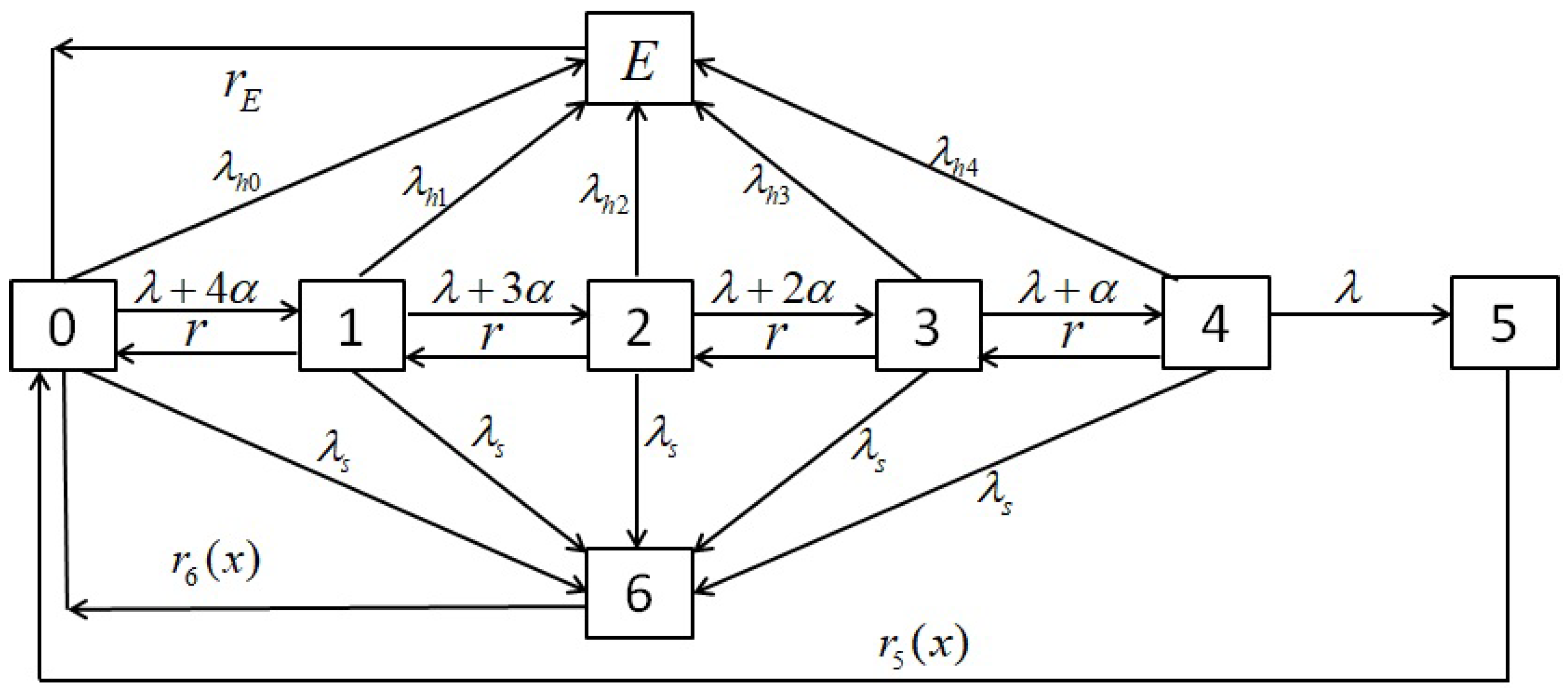
• State 0: One robot and the safety device in the five-robot system are functioning normally, while four robots remain in hot standby status.
• State 1: One robot and the safety device in the five-robot system are functioning normally, one robot has malfunctioned, and three robots are in a hot standby status.
• State 2: One robot and the safety device in the five-robot system are functioning normally, two robots have malfunctioned, and two robots are in a hot standby status.
• State 3: One robot and the safety device in the five-robot system are functioning normally, three robots have malfunctioned, and one robot is in a hot standby status.
• State 4: One robot and the safety device in the system are functioning normally, while four robots have malfunctioned.
• State 5: The state of the five-robot system is due to the malfunction of all five robots.
• State 6: The state of the five-robot system is a result of the malfunction of the safety device.
• State E: The state of the five-robot system resulting from routine failures.

Based on the aforementioned assumptions, it is evident that $\left\{N\right(t),t\ge 0\}$ does not constitute a Markov process. Nevertheless, we can employ the method of supplementary variables to convert it into a high-dimensional Markov process (see [13]), as outlined below.

The state transition diagram of the five-robot system is presented in Figure 1.

Assume that the malfunctioning five-robot system is in a maintenance state. Let $X_j\left(t\right)(j=5,6)$ denote the maintenance time utilized from the commencement of maintenance until the present time, and let

$$\begin{array}{c}\hfill Z\left(t\right)=\left\{\begin{array}{c}N\left(t\right),N\left(t\right)=0,1,2,3,4,E,\hfill \\ (N\left(t\right),X_5\left(t\right)),N\left(t\right)=5,\hfill \\ (N\left(t\right),X_6\left(t\right)),N\left(t\right)=6.\hfill \end{array}\right.\end{array}$$

It is evident that $\left\{Z\right(t),t\ge 0\}$ constitutes a Markov process. Let $P_i\left(t\right)(i=0,1,2,3,4,E)$ denote the probability that the five-robot system occupies state i at time t; $P_j(t,x)(j=5,6)$ denotes the probability density that the five-robot system occupies state j at time t and that the elapsed repair time x lies within the interval $(x,x+dx)$, namely,

$$\begin{array}{c}\hfill \left\{\begin{array}{c}{P}_0\left(t\right)=P\{N\left(t\right)=0\},\hfill \\ P_1\left(t\right)=P\{N\left(t\right)=1\},\hfill \\ P_2\left(t\right)=P\{N\left(t\right)=2\},\hfill \\ P_3\left(t\right)=P\{N\left(t\right)=3\},\hfill \\ P_4\left(t\right)=P\{N\left(t\right)=4\},\hfill \\ P_E\left(t\right)=P\{N\left(t\right)=E\},\hfill \\ P_5(t,x)dx=P\{x<X_5\left(t\right)\le x+dx,N\left(t\right)=5\},\hfill \\ P_6(t,x)dx=P\{x<X_6\left(t\right)\le x+dx,N\left(t\right)=6\}.\hfill \end{array}\right.\end{array}$$

2.2. Notation

The following symbols associated with Figure 1 or its related analyses:

• t denotes time.
• i denotes the ith state of the five-robot system.
• $P_i\left(t\right)$ denotes the probability that the five-robot system occupies state i, for $i=0,1,2,3,4,E,5,6$, at time t.
• $P_j(t,x)dx$ denotes the probability that, at time t, the failed five-robot system in state $j(j=5,6)$ is undergoing repair and that the elapsed repair time falls within the interval $(x,x+dx)$, where $(t,x)\in [0,\infty )\times [0,\infty )$.
• $P_i$ denotes the steady-state probability that the five-robot system occupies state i, for $i=0,1,2,3,4,E$.
• $\lambda$ denotes the constant damage rate resulting from the robot’s inherent factors.
• ${\lambda }_{hi}$ denotes the constant normal damage rate from states $i(i=0,1,2,3,4)$ to state E.
• ${\lambda }_s$ denotes the constant human-induced failure rate of the work system transitioning from states $i(i=0,1,2,3,4)$ to state 6.
• $\alpha$ denotes the constant damage rate of thermal reserve robots.
• r denotes the constant repair rate of normal working robots transitioning from state $i+1$ to state i$(i=0,1,2,3)$.
• $r_E$ denotes the constant repair rate of the operating system transitioning from state E to state 0.
• $r_j\left(x\right)$ denotes the repair rates from state $j(j=5,6)$ to state 0. It satisfies the conditions: $0<\underset{x\ge 0}{inf}{r}_j\left(x\right)<\underset{x\ge 0}{sup}{r}_j\left(x\right)<+\infty ,M=max\{\underset{x\ge 0}{sup}{r}_j\left(x\right),j=5,6\},{\int }_0^{\mathrm{T}}{r}_j\left(x\right)dx<+\infty (0<\mathrm{T}<+\infty ),$ ${\int }_0^{+\infty }{e}^{-{\int }_0^x{r}_j\left(\tau \right)d\tau }dx<+\infty$,${\int }_0^{+\infty }{r}_j\left(x\right)dx<+\infty$, and $0<\underset{x\to +\infty }{lim}{\displaystyle \frac{1}{x}}$${\int }_0^x{r}_j\left(\tau \right)d\tau =r_j<+\infty ,j=5,6$. Additionally, $\overline{r}=min\{r_5,r_6\}$.

2.3. Formulation of the Five-Robot System Model

Using the notation described above and the state space diagram of the five-robot system model presented in Figure 1, we can apply the law of total probability to obtain

$$\begin{array}{ccc}& & P_0(t+▵t)=(1-a_0▵t)P_0\left(t\right)+r{P}_1\left(t\right)▵t+r_E{P}_E\left(t\right)▵t+\sum _{j=5}^6{\int }_0^{+\infty }{P}_j(t,x)r_j\left(x\right)▵tdx+o(▵t),\hfill \\ & & P_1(t+▵t)=(1-a_1▵t)P_1\left(t\right)+(\lambda +4\alpha )P_0\left(t\right)▵t+r{P}_2\left(t\right)▵t+o(▵t),\hfill \\ & & P_2(t+▵t)=(1-a_2▵t)P_2\left(t\right)+(\lambda +3\alpha )P_1\left(t\right)▵t+r{P}_3\left(t\right)▵t+o(▵t),\hfill \\ & & P_3(t+▵t)=(1-a_3▵t)P_3\left(t\right)+(\lambda +2\alpha )P_2\left(t\right)▵t+r{P}_4\left(t\right)▵t+o(▵t),\hfill \\ & & P_4(t+▵t)=(1-a_4▵t)P_4\left(t\right)+(\lambda +\alpha )P_3\left(t\right)▵t+o(▵t),\hfill \\ & & P_E(t+▵t)=(1-r_E▵t)P_E\left(t\right)+{\lambda }_{h0}{P}_0\left(t\right)▵t+{\lambda }_{h1}{P}_1\left(t\right)▵t+{\lambda }_{h2}{P}_2\left(t\right)▵t+{\lambda }_{h3}{P}_3\left(t\right)▵t\hfill \\ & & +{\lambda }_{h4}{P}_4\left(t\right)▵t+o(▵t),\hfill \\ & & P_j(t+▵t,x+▵x)=\left(1-r_j\left(x\right)▵t\right)P_j(t,x)+o(▵t)(j=5,6),\hfill \end{array}$$

where

$a_0=\lambda +4\alpha +{\lambda }_{h0}+{\lambda }_s$,

$a_1=r+\lambda +3\alpha +{\lambda }_{h1}+{\lambda }_s$,

$a_2=r+\lambda +2\alpha +{\lambda }_{h2}+{\lambda }_s$,

$a_3=r+\lambda +\alpha +{\lambda }_{h3}+{\lambda }_s$,

$a_4=r+\lambda +{\lambda }_{h4}+{\lambda }_s$.

To facilitate the discussion of the system’s stability, reliability, and numerical simulation in the subsequent text, the preceding expression is reorganized. Let $▵t\to 0$. Based on probability analysis, the system of integral and differential equations related to the model depicted in Figure 1 is derived as follows (see [14,15,16]):

$$\begin{array}{lll}& & {\displaystyle \frac{d}{dt}}{P}_0\left(t\right)=-a_0{P}_0\left(t\right)+r{P}_1\left(t\right)+r_E{P}_E\left(t\right)+\sum _{i=5}^6{\int }_0^{+\infty }{P}_i(t,x)r_i\left(x\right)dx,\hfill \end{array}$$

(1)

$$\begin{array}{lll}& & {\displaystyle \frac{d}{dt}}{P}_1\left(t\right)=-a_1{P}_1\left(t\right)+(\lambda +4\alpha )P_0\left(t\right)+r{P}_2\left(t\right),\hfill \end{array}$$

(2)

$$\begin{array}{lll}& & {\displaystyle \frac{d}{dt}}{P}_2\left(t\right)=-a_2{P}_2\left(t\right)+(\lambda +3\alpha )P_1\left(t\right)+r{P}_3\left(t\right),\hfill \end{array}$$

(3)

$$\begin{array}{lll}& & {\displaystyle \frac{d}{dt}}{P}_3\left(t\right)=-a_3{P}_3\left(t\right)+(\lambda +2\alpha )P_2\left(t\right)+r{P}_4\left(t\right),\hfill \end{array}$$

(4)

$$\begin{array}{lll}& & {\displaystyle \frac{d}{dt}}{P}_4\left(t\right)=-a_4{P}_4\left(t\right)+(\lambda +\alpha )P_3\left(t\right),\hfill \end{array}$$

(5)

$$\begin{array}{lll}& & {\displaystyle \frac{d}{dt}}{P}_E\left(t\right)={\lambda }_{h0}{P}_0\left(t\right)+{\lambda }_{h1}{P}_1\left(t\right)+{\lambda }_{h2}{P}_2\left(t\right)+{\lambda }_{h3}{P}_3\left(t\right)+{\lambda }_{h4}{P}_4\left(t\right)-r_E{P}_E\left(t\right),\hfill \end{array}$$

(6)

$$\begin{array}{lll}& & {\displaystyle \frac{\partial }{\partial x}}{P}_i(t,x)+{\displaystyle \frac{\partial }{\partial t}}{P}_i(t,x)=-r_i\left(x\right)P_i(t,x)(i=5,6),\hfill \end{array}$$

(7)

$$\mathrm{Boundary}\mathrm{conditions}:$$

$$\begin{array}{lll}& & P_5(t,0)=\lambda P_4\left(t\right),\hfill \end{array}$$

(8)

$$\begin{array}{lll}& & P_6(t,0)={\lambda }_s\sum _{i=0}^4{P}_i\left(t\right),\hfill \end{array}$$

(9)

$$\mathrm{Initial}\mathrm{conditions}:$$

$$\begin{array}{lll}& & P_0\left(0\right)=1,\hfill \end{array}$$

(10)

$$\begin{array}{lll}& & P_1\left(0\right)=P_2\left(0\right)=P_3\left(0\right)=P_4\left(0\right)=P_E\left(0\right)=P_5(0,x)=P_6(0,x)=0.\hfill \end{array}$$

(11)

where $a_0=\lambda +4\alpha +{\lambda }_{h0}+{\lambda }_s,a_1=r+\lambda +3\alpha +{\lambda }_{h1}+{\lambda }_s,a_2=r+\lambda +2\alpha +{\lambda }_{h2}+{\lambda }_s,a_3=r+\lambda +\alpha +{\lambda }_{h3}+{\lambda }_s,a_4=r+\lambda +{\lambda }_{h4}+{\lambda }_s$.

3. Stability Analysis

3.1. Constructing the System Model Based on the Abstract Cauchy Problem

To facilitate the discussion of subsequent issues, we will reformulate the Equations (1)–() that describe the system state into an abstract Cauchy problem within a Banach space.

Initially, let $\mathbb{R}$ represent the set of real numbers, ${\mathbb{R}}^{+}$ denote the set of positive real numbers, $L^1\left({\mathbb{R}}^{+}\right)$ denote the Lebesgue integrable space on the set of positive real numbers, $L^{\infty }\left({\mathbb{R}}^{+}\right)$ denote the dual space of $L^1\left({\mathbb{R}}^{+}\right)$, and let X be defined as the state space:

$$X\triangleq \left\{\mathit{P}|\mathit{P}\in {\mathbb{R}}^6\times L^1\left({\mathbb{R}}^{+}\right)\times L^1\left({\mathbb{R}}^{+}\right),\left|\right|\mathit{P}\left|\right|<\infty \right\},$$

where

$\mathit{P}\triangleq {\left(P_0,P_1,P_2,P_3,P_4,P_E,P_5\left(x\right),P_6\left(x\right)\right)}^T,$

$\left|\right|\mathit{P}\left|\right|=|P_0|+|P_1|+|P_2|+|P_3|+|P_4|+|P_E|+||P_5{\left|\right|}_{L^1\left({\mathbb{R}}^{+}\right)}+\left|\right|P_6{\left|\right|}_{L^1\left({\mathbb{R}}^{+}\right)}$.

Verifying that $(X,\parallel ·\parallel )$ is a Banach space is straightforward.

Next, let us define the operators $\mathit{B}$ and $\mathit{U}$ as follows:

$$\begin{array}{ccc}& & \mathit{B}=\left(\begin{array}{cccccccc}-a_0& & & & & & & \\ & -a_1& & & & & & \\ & & -a_2& & & & & \\ & & & -a_3& & & & \\ & & & & -a_4& & & \\ & & & & & -r_E& & \\ & & & & & & -{\displaystyle \frac{\partial }{\partial x}}-r_5\left(x\right)& \\ & & & & & & & -{\displaystyle \frac{\partial }{\partial x}}-r_6\left(x\right)\end{array}\right),\hfill \\ & & \mathit{U}\mathit{P}=\left(\begin{array}{cccccccc}0& r{P}_1& 0& 0& 0& r_E{P}_E& {\int }_0^{\infty }{r}_5\left(x\right)P_5\left(x\right)dx& {\int }_0^{\infty }{r}_6\left(x\right)P_6\left(x\right)dx\\ (\lambda +4\alpha )P_0& 0& r{P}_2& 0& 0& 0& 0& 0\\ 0& (\lambda +3\alpha )P_1& 0& r{P}_4& 0& 0& 0& 0\\ 0& 0& (\lambda +2\alpha )P_2& 0& r& 0& 0& 0\\ 0& 0& 0& (\lambda +\alpha )P_3& 0& 0& 0& 0\\ {\lambda }_{h0}{P}_0& {\lambda }_{h1}{P}_1& {\lambda }_{h2}{P}_2& {\lambda }_{h3}{P}_3& {\lambda }_{h4}{P}_4& 0& 0& 0\\ 0& 0& 0& 0& 0& 0& 0& 0\\ 0& 0& 0& 0& 0& 0& 0& 0\end{array}\right),\hfill \end{array}$$

$D\left(\mathit{B}\right)=\{\mathit{P}\in X|{\displaystyle \frac{\partial }{\partial x}}{P}_i(t,x)+r_i\left(x\right)P_i(t,x)\in L^1\left({\mathbb{R}}^{+}\right),P_i(t,x)(i=5,6)$ is an absolutely continuous function and satisfies $P_5(t,0)=\lambda P_4\left(t\right),P_6(t,0)={\lambda }_s{\displaystyle \sum _{i=0}^4}{P}_i\left(t\right)\},$ $D\left(\mathit{U}\right)=X.$

Therefore, the Equations (1)–(11) that describe the five-robot system can be transformed into an abstract Cauchy problem in Banach space (see [17]) (ACP):

$$\begin{array}{c}\hfill \left.\begin{array}{c}{\displaystyle \frac{\partial }{\partial t}}\mathit{P}(t,·)=(\mathit{B}+\mathit{U})\mathit{P}(t,·),t\ge 0,\hfill \\ \mathit{P}(0,·)={\mathit{P}}^0,\hfill \\ \mathit{P}(t,·)\triangleq {\left(P_0\left(t\right),P_1\left(t\right),P_2\left(t\right),P_3\left(t\right),P_4\left(t\right),P_E\left(t\right),P_5(t,·),P_6(t,·)\right)}^T\hfill \end{array}\right\}\end{array}$$

(12)

where ${\mathit{P}}^0={(1,0,0,0,0,0,0,0)}^T$.

3.2. The Well-Posedness Analysis

In this subsection, we employ analytical methods to establish the existence and uniqueness of classical solutions for the five-robot system (1)–(11).

Theorem 1. 

When $\mathrm{T}>0$, the five-robot system (1)–(11) possesses a unique non-negative classical solution in $C[0,\mathrm{T}]$.

Proof. 

By employing the method of characteristics (see [18]), the solution of (7) can be obtained as follows.

$$\begin{array}{c}\hfill P_i(t,x)=P_i(t-x,0)e^{-{\int }_0^x{r}_i\left(s\right)ds}(i=5,6).\end{array}$$

(13)

Substituting Equation (13) into Equation (1) yields,

$$\begin{array}{ccc}& & P_0\left(t\right)=e^{-a_{0}t}+{\int }_0^{t}r{e}^{-a_0(t-\eta )}{P}_1\left(\eta \right)d\eta +{\int }_0^t{r}_E{e}^{-a_0(t-\eta )}{P}_E\left(\eta \right)d\eta \hfill \\ & & +\sum _{i=5}^6{\int }_0^t{k}_i(t-\eta )P_i(\eta ,0)d\eta ,\hfill \end{array}$$

(14)

where

$k_i(t-\eta )={\int }_0^{t-\eta }{e}^{-a_0(t-\eta )}{e}^{a_{0}v-{\int }_0^v{r}_i\left(\eta \right)d\eta }{r}_i\left(v\right)dv,i=5,6.$

The solution to Equations (2) through (6) yields,

$$\begin{array}{ccc}& & P_1\left(t\right)={\int }_0^t(\lambda +4\alpha )e^{-a_1(t-\eta )}{P}_0\left(\eta \right)d\eta +{\int }_0^{t}r{e}^{-a_1(t-\eta )}{P}_2\left(\eta \right)d\eta ,\hfill \end{array}$$

(15)

$$\begin{array}{ccc}& & P_2\left(t\right)={\int }_0^t(\lambda +3\alpha )e^{-a_2(t-\eta )}{P}_1\left(\eta \right)d\eta +{\int }_0^{t}r{e}^{-a_2(t-\eta )}{P}_3\left(\eta \right)d\eta ,\hfill \end{array}$$

(16)

$$\begin{array}{ccc}& & P_3\left(t\right)={\int }_0^t(\lambda +2\alpha )e^{-a_3(t-\eta )}{P}_2\left(\eta \right)d\eta +{\int }_0^{t}r{e}^{-a_3(t-\eta )}{P}_4\left(\eta \right)d\eta ,\hfill \end{array}$$

(17)

$$\begin{array}{ccc}& & P_4\left(t\right)={\int }_0^t(\lambda +\alpha )e^{-a_4(t-\eta )}{P}_3\left(\eta \right)d\eta ,\hfill \end{array}$$

(18)

$$\begin{array}{ccc}& & P_E\left(t\right)={\int }_0^t{\lambda }_{h0}{e}^{-r_E(t-\eta )}{P}_0\left(\eta \right)d\eta +{\int }_0^t{\lambda }_{h1}{e}^{-r_E(t-\eta )}{P}_1\left(\eta \right)d\eta +{\int }_0^t{\lambda }_{h2}{e}^{-r_E(t-\eta )}{P}_2\left(\eta \right)d\eta \hfill \\ & & +{\int }_0^t{\lambda }_{h3}{e}^{-r_E(t-\eta )}{P}_3\left(\eta \right)d\eta +{\int }_0^t{\lambda }_{h4}{e}^{-r_E(t-\eta )}{P}_4\left(\eta \right)d\eta .\hfill \end{array}$$

(19)

Substituting Equations (18) and (14)–(18) into Equations (8) and (9) respectively yields,

$$\begin{array}{ccc}& & P_5(t,0)={\int }_0^t\lambda (\lambda +\alpha )e^{-a_4(t-\eta )}{P}_3\left(\eta \right)d\eta ,\hfill \end{array}$$

(20)

$$\begin{array}{ccc}& & P_6(t,0)={\lambda }_s{e}^{-a_{0}t}+{\int }_0^t{\lambda }_s(\lambda +4\alpha )e^{-a_1(t-\eta )}{P}_0\left(\eta \right)d\eta \hfill \\ & & +{\int }_0^t{\lambda }_s[(\lambda +3\alpha )e^{-a_2(t-\eta )}+r{e}^{-a_0(t-\eta )}]P_1\left(\eta \right)d\eta \hfill \\ & & +{\int }_0^t{\lambda }_s[(\lambda +2\alpha )e^{-a_3(t-\eta )}+r{e}^{-a_1(t-\eta )}]P_2\left(\eta \right)d\eta \hfill \\ & & +{\int }_0^t{\lambda }_s[(\lambda +\alpha )e^{-a_4(t-\eta )}+r{e}^{-a_2(t-\eta )}]P_3\left(\eta \right)d\eta +{\int }_0^t{\lambda }_{s}r{e}^{-a_3(t-\eta )}{P}_4\left(\eta \right)d\eta \hfill \\ & & +{\int }_0^t{\lambda }_s{r}_E{e}^{-a_0(t-\eta )}{P}_E\left(\eta \right)d\eta +\sum _{i=5}^6{\int }_0^t{\lambda }_s{k}_i(t-\eta )P_i(\eta ,0)d\eta .\hfill \end{array}$$

(21)

Combining the Equations (14)–(21) results in a convolution-type Volterra integral equation system (VIE), which can be expressed in vector form as follows:

$$\begin{array}{c}\hfill \left(\mathrm{VIE}\right)\mathit{P}\left(t\right)=\mathit{H}\left(t\right)+{\int }_0^t\mathit{K}(t-\eta )\mathit{P}\left(\eta \right)d\eta ,\end{array}$$

(22)

where

$\mathit{P}\left(t\right)={\left(P_0\left(t\right),P_1\left(t\right),P_2\left(t\right),P_3\left(t\right),P_4\left(t\right),P_E\left(t\right),P_5(t,0),P_6(t,0)\right)}^T$,

$\mathit{H}\left(t\right)={(e^{-a_{0}t},0,0,0,0,0,0,{\lambda }_s{e}^{-a_{0}t})}^T$,

$\mathit{K}(t-\eta )=\left(\begin{array}{cccccccc}0& {\displaystyle \frac{k_0}{r_E}}& 0& 0& 0& {\displaystyle \frac{k_0}{r}}& k_5& k_6\\ {\displaystyle \frac{k_1}{r}}& 0& {\displaystyle \frac{k_1}{(\lambda +4\alpha )}}& 0& 0& 0& 0& 0\\ 0& {\displaystyle \frac{k_2}{r}}& 0& {\displaystyle \frac{k_2}{(\lambda +3\alpha )}}& 0& 0& 0& 0\\ 0& 0& {\displaystyle \frac{k_3}{r}}& 0& {\displaystyle \frac{k_3}{\lambda +2\alpha }}& 0& 0& 0\\ 0& 0& 0& {\displaystyle \frac{k_4}{r}}& 0& 0& 0& 0\\ {\lambda }_{h0}{k}_E& {\lambda }_{h1}{k}_E& {\lambda }_{h2}{k}_E& {\lambda }_{h3}{k}_E& {\lambda }_{h4}{k}_E& 0& 0& 0\\ 0& 0& 0& {\displaystyle \frac{\lambda k_4}{r}}& 0& 0& 0& 0\\ {\displaystyle \frac{{\lambda }_s{k}_1}{r}}& {\displaystyle \frac{{\lambda }_s{k}_2}{r}}+{\displaystyle \frac{{\lambda }_s{k}_0}{r_E}}& {\displaystyle \frac{{\lambda }_s{k}_3}{r}}+{\displaystyle \frac{{\lambda }_s{k}_1}{\lambda +4\alpha }}& {\displaystyle \frac{{\lambda }_s{k}_4}{r}}+{\displaystyle \frac{{\lambda }_s{k}_2}{\lambda +3\alpha }}& {\displaystyle \frac{{\lambda }_s{k}_3}{\lambda +2\alpha }}& {\displaystyle \frac{{\lambda }_s{k}_0}{r}}& {\lambda }_s{k}_4& {\lambda }_s{k}_5\end{array}\right)$,

$k_0=r{r}_E{e}^{-a_0(t-\eta )}$,

$k_1=(\lambda +4\alpha )r{e}^{-a_1(t-\eta )}$,

$k_2=(\lambda +3\alpha )r{e}^{-a_2(t-\eta )}$,

$k_3=(\lambda +2\alpha )r{e}^{-a_3(t-\eta )}$,

$k_4=(\lambda +\alpha )r{e}^{-a_4(t-\eta )}$,

$k_E=e^{-r_E(t-\eta )}$,

$k_i={\int }_0^{t-\eta }{e}^{-a_0(t-\eta )}{e}^{a_{0}v-{\int }_0^v{r}_i\left(\eta \right)d\eta }{r}_i\left(v\right)dv,i=5,6.$

Based on the preceding discussion, the existence and uniqueness of non-negative classical solutions for the Equations (1)–(11) that describe the five-robot system are equivalent to the existence of non-negative classical solutions for the Volterra integral equation (VIE). It is important to note that each component of $\mathit{H}\left(t\right)$ and $\mathit{K}(t-\eta )$ is a non-negative and bounded function. For all $\mathrm{T}>0$, the function is also absolutely integrable on $C[0,\mathrm{T}]$. Therefore, it can be concluded that a classical solution to the Volterra integral equation (VIE) exists in $C[0,\mathrm{T}]$.

The solution is both non-negative and unique, which implies that for all $\mathrm{T}>0$, there exists a unique non-negative classical solution to the five-robot system (1)–(11) in $C[0,\mathrm{T}]$ (see [19]). □

3.3. Asymptotic Stability

Formulate an abstract Cauchy problem (ACP) associated with the main operator $\mathit{B}+\mathit{U}$ in a suitable space. This section aims to analyze the asymptotic stability of the five-robot system by demonstrating that the main operator $\mathit{B}+\mathit{U}$ in Equation (12) generates a $C_0$-semigroup $\left\{S\right(t\left)\right|t\ge 0\}$.

Definition 1. 

Let X be a Banach space. A one parameter family $T\left(t\right),0\le t<\infty$, of bounded linear operators from X to X is a semigroup of bounded linear operators on X if (see [17])

$$\begin{array}{ccc}& & \left(I\right)T\left(0\right)=I\left(I\mathit{is}\mathit{the}\mathit{identity}\mathit{operator}\mathit{on}X\right).\hfill \\ & & \left(II\right)T(t+s)=T\left(t\right)T\left(s\right)\mathit{for}\mathit{very}t,s\ge 0\left(\mathit{the}\mathit{semigroup}\mathit{property}\right).\hfill \end{array}$$

Theorem 2. 

The simple eigenvalue of the primary operator $\mathit{B}+\mathit{U}$ for the five-robot system (12) is 0.

Proof. 

Assume that $\mathit{P}$ satisfies Equations (8)–(11).Consider the equation $(\mathit{B}+\mathit{U})\mathit{P}=0$. We have

$$\begin{array}{ccc}& & a_0{P}_0-r{P}_1-r_E{P}_E-\sum _{i=5}^6{\int }_0^{\infty }{P}_i\left(x\right)r_i\left(x\right)dx=0,\hfill \end{array}$$

(23)

$$\begin{array}{ccc}& & a_1{P}_1-(\lambda +4\alpha )P_0-r{P}_2=0,\hfill \end{array}$$

(24)

$$\begin{array}{ccc}& & a_2{P}_2-(\lambda +3\alpha )P_1-r{P}_3=0,\hfill \end{array}$$

(25)

$$\begin{array}{ccc}& & a_3{P}_3-(\lambda +2\alpha )P_2-r{P}_4=0,\hfill \end{array}$$

(26)

$$\begin{array}{ccc}& & a_4{P}_4-(\lambda +\alpha )P_3=0,\hfill \end{array}$$

(27)

$$\begin{array}{ccc}& & r_E{P}_E-{\lambda }_{h0}{P}_0-{\lambda }_{h1}{P}_1-{\lambda }_{h2}{P}_2-{\lambda }_{h3}{P}_3-{\lambda }_{h4}{P}_4=0,\hfill \end{array}$$

(28)

$$\begin{array}{ccc}& & {\displaystyle \frac{d{P}_i\left(x\right)}{dx}}+r_i\left(x\right)P_i\left(x\right)=0(i=5,6),\hfill \end{array}$$

(29)

$$\begin{array}{ccc}& & P_5\left(0\right)=\lambda P_4,\hfill \end{array}$$

(30)

$$\begin{array}{ccc}& & P_6\left(0\right)={\lambda }_s\sum _{i=0}^4{P}_i.\hfill \end{array}$$

(31)

Solve the Equations (29)–(31) to obtain

$$\begin{array}{c}\hfill P_i\left(x\right)=P_i\left(0\right)e^{-{\int }_0^x{r}_i\left(\eta \right)d\eta }(i=5,6).\end{array}$$

(32)

Substituting Equation (32) into Equation (23) and combining it with Equations (24)–(28) yields

$$\begin{array}{ccc}& & (a_0-{\lambda }_s)P_0-(r+{\lambda }_s)P_1-{\lambda }_s{P}_2-{\lambda }_s{P}_3-(\lambda +{\lambda }_s)P_4-r_E{P}_E=0,\hfill \\ & & (\lambda +4\alpha )P_0-a_1{P}_1+r{P}_2=0,\hfill \\ & & (\lambda +3\alpha )P_1-a_2{P}_2+r{P}_3=0,\hfill \\ & & (\lambda +2\alpha )P_2-a_3{P}_3+r{P}_4=0,\hfill \\ & & (\lambda +\alpha )P_3-a_4{P}_4=0,\hfill \\ & & r_E{P}_E-{\lambda }_{h0}{P}_0-{\lambda }_{h1}{P}_1-{\lambda }_{h2}{P}_2-{\lambda }_{h3}{P}_3-{\lambda }_{h4}{P}_4=0.\hfill \end{array}$$

Based on the preceding verification, it is evident that the value of the coefficient determinant for the aforementioned system of equations is equal to zero. Furthermore, when $P_0>0$, $P_1,P_2,P_3,P_4,P_E$ are all greater than zero. Furthermore, from the expressions of $P_0$ and $a_0,a_1,a_2,a_3,a_4$, it can be inferred that $P_i\left(x\right)$ for $i=5,6$ are all non-negative. Therefore, we have the vector

$$\begin{array}{c}\hfill {\mathit{P}}^{*}={\left(P_0,P_1,P_2,P_3,P_4,P_E,P_5\left(x\right),P_6\left(x\right)\right)}^T\end{array}$$

(33)

(where $P_i$ for $i=0,1,2,3,4,E$, as well as $P_5\left(x\right)$ and $P_6\left(x\right)$, are defined by Equations (23)–(32).) is the non-negative eigenvector corresponding to the 0 eigenvalue of the main operator $\mathit{B}+\mathit{U}$ for the five-robot system (12), and it also represents the steady-state solution of the Equation (12).

Let $\mathit{q}=(1,1,1,1,1,1,1,1)$ represent an arbitrary selection. Then, we have

$$<{\mathit{P}}^{*},\mathit{q}>=\sum _{i=0}^4{P}_i+P_E+\sum _{i=5}^6{\int }_0^{\infty }{P}_i\left(x\right)dx>0,$$

and for any ${\mathit{P}}^{*}\in D(\mathit{B}+\mathit{U})=D\left(\mathit{B}\right)\bigcap D\left(\mathit{U}\right)$, we perform the inner product operation $<(\mathit{B}+\mathit{U}){\mathit{P}}^{*},\mathit{q}>=0$. We conclude that 0 is a simple eigenvalue of the main operator $\mathit{B}+\mathit{U}$. □

Below, for the convenience of discussing the issues later, we present several useful lemmas.

Lemma 1. 

Let the operator $\mathit{A}$ be a dense resolvent operator. If $D{\left(\mathit{A}\right)}_{+}$ is cofinal in ${\mathbb{E}}_{+}$, or in ${\mathbb{E}}_{+}^{*}$, then $\mathit{A}$ is the generator of a positive $C_0$-semigroup, and it holds that $s\left(\mathit{A}\right)=\omega \left(\mathit{A}\right)$ (see [20]).

Lemma 2. 

There exists a positive constant $N_2$ such that for any $t\ge 0$ (see [21]),

$${\int }_t^{\infty }{e}^{-{\int }_t^{x}r\left(s\right)ds}dx\le N_2.$$

Lemma 3. 

For any $\gamma \in \left\{\gamma \in \mathbb{C}|\mathbf{Re}\gamma >0\mathrm{or}\gamma =\mathrm{i}a,a\in \mathbb{R}\setminus \{0\}\right\}$, $r\left(x\right)\ge 0$, then (see [22])

$$\left|{\int }_0^{\infty }r\left(x\right)e^{-{\int }_0^x[\gamma +r\left(s\right)]ds}dx\right|<1.$$

Lemma 4. 

The primary operator $\mathit{B}+\mathit{U}$ of the five-robot system (12) is a densely dissipative operator (see [23]).

Lemma 5. 

The set $\left\{\gamma \in \mathbb{C}|\mathbf{Re}\gamma >0\mathrm{or}\gamma =\mathrm{i}b,b\in \mathbb{R}\setminus \{0\}\right\}$ is contained in $\rho (\mathit{B}+\mathit{U})$.

Proof. 

Firstly, for any $G=(g_0,g_1,g_2,g_3,g_4,g_E,g_5\left(x\right),g_6\left(x\right))\in X$, considering the equation $[\gamma I-(\mathit{B}+\mathit{U}\left)\right]\mathit{P}=G$. That is

$$\begin{array}{ccc}& & (\gamma +a_0)P_0-r{P}_1-r_E{P}_E-\sum _{i=5}^6{\int }_0^{\infty }{P}_i\left(x\right)r_i\left(x\right)dx=g_0,\hfill \end{array}$$

(34)

$$\begin{array}{ccc}& & (\gamma +a_1)P_1-(\lambda +4\alpha )P_0-r{P}_2=g_1,\hfill \end{array}$$

(35)

$$\begin{array}{ccc}& & (\gamma +a_2)P_2-(\lambda +3\alpha )P_1-r{P}_3=g_2,\hfill \end{array}$$

(36)

$$\begin{array}{ccc}& & (\gamma +a_3)P_3-(\lambda +2\alpha )P_2-r{P}_4=g_3,\hfill \end{array}$$

(37)

$$\begin{array}{ccc}& & (\gamma +a_4)P_4-(\lambda +\alpha )P_3=g_4,\hfill \end{array}$$

(38)

$$\begin{array}{ccc}& & (\gamma +r_E)P_E-{\lambda }_{h0}{P}_0-{\lambda }_{h1}{P}_1-{\lambda }_{h2}{P}_2-{\lambda }_{h3}{P}_3-{\lambda }_{h4}{P}_4=g_E,\hfill \end{array}$$

(39)

$$\begin{array}{ccc}& & {\displaystyle \frac{d{P}_j\left(x\right)}{dx}}+(\gamma +r_j\left(x\right))P_j\left(x\right)=g_j\left(x\right)(j=5,6).\hfill \end{array}$$

(40)

And we can suppose

$$\begin{array}{ccc}& & P_5\left(0\right)=\lambda P_4,\hfill \end{array}$$

(41)

$$\begin{array}{ccc}& & P_6\left(0\right)={\lambda }_s\sum _{i=0}^4{P}_i.\hfill \end{array}$$

(42)

Solving (40) with the help of (41)–(42) gets

$$\begin{array}{ccc}& & P_j\left(x\right)=P_j\left(0\right)e^{-{\int }_0^x[\gamma +r_j\left(s\right)]ds}+{\int }_0^x{e}^{-{\int }_{\tau }^x[\gamma +r_j\left(s\right)]ds}{g}_j\left(\tau \right)d\tau .\hfill \end{array}$$

(43)

Noticing that $g_j\left(x\right)\in L^1\left({\mathbb{R}}^{+}\right),j=5,6$, together with Lemma 2, we know $P_j\left(x\right)\in L^1\left({\mathbb{R}}^{+}\right),j=5,6$. This implies that $[\gamma I-(\mathit{B}+\mathit{U}\left)\right]$ is an onto mapping.

Secondly, we will prove that this operator is also an injective mapping. That is, the operator equation $[\gamma I-(\mathit{B}+\mathit{U}\left)\right]P=0$ has a unique solution 0. Set $G=0$ in the former discussion. Then we can obtain the following matrix equation by combing (34)–(39) with (43),

$$\begin{array}{c}\hfill \left(\begin{array}{cccccc}\gamma +a_0& -(r+{\lambda }_s{W}_6)& -{\lambda }_s{W}_6& -{\lambda }_s{W}_6& -(\lambda W_5+{\lambda }_s{W}_6)& -r_E\\ -(\lambda +4\alpha )& \gamma +a_1& -r& 0& 0& 0\\ 0& -(\lambda +3\alpha )& \gamma +a_2& -r& 0& 0\\ 0& 0& -(\lambda +2\alpha )& \gamma +a_3& -r& 0\\ 0& 0& 0& -(\lambda +\alpha )& \gamma +a_4& 0\\ -{\lambda }_{h0}& -{\lambda }_{h1}& -{\lambda }_{h2}& -{\lambda }_{h3}& -{\lambda }_{h4}& \gamma +r_E\end{array}\right)\left(\begin{array}{c}{P}_0\\ P_1\\ P_2\\ P_3\\ P_4\\ P_E\end{array}\right)=\left(\begin{array}{c}0\\ 0\\ 0\\ 0\\ 0\\ 0\end{array}\right),\end{array}$$

(44)

where $W_j={\int }_0^{\infty }{r}_j\left(x\right)e^{-{\int }_0^x[\gamma +r_j\left(\tau \right)]d\tau }dx,j=5,6$.

It is clear that

$|\gamma +a_0|=|\gamma +\lambda +4\alpha +{\lambda }_{h0}+{\lambda }_s|>|\lambda +4\alpha +{\lambda }_{h0}|,$

$|\gamma +a_1|=|\gamma +r+\lambda +3\alpha +{\lambda }_{h1}+{\lambda }_s|>|r+\lambda +3\alpha +{\lambda }_{h1}+{\lambda }_s|>|r+\lambda +3\alpha +{\lambda }_{h1}+{\lambda }_s{W}_6|,$

$|\gamma +a_2|=|\gamma +r+\lambda +2\alpha +{\lambda }_{h2}+{\lambda }_s|>|r+\lambda +2\alpha +{\lambda }_{h2}+{\lambda }_s|>|r+\lambda +2\alpha +{\lambda }_{h2}+{\lambda }_s{W}_6|,$

$|\gamma +a_3|=|\gamma +r+\lambda +\alpha +{\lambda }_{h3}+{\lambda }_s|>|r+\lambda +\alpha +{\lambda }_{h3}+{\lambda }_s|>|r+\lambda +\alpha +{\lambda }_{h3}+{\lambda }_s{W}_6|,$

$|\gamma +a_4|=|\gamma +r+\lambda +{\lambda }_{h4}+{\lambda }_s|>|r+\lambda +{\lambda }_{h4}+{\lambda }_s|>|r+\lambda W_5+{\lambda }_{h4}+{\lambda }_s{W}_6|,$$|\gamma +r_E|>|r_E|$, for $\gamma >0$ or $\gamma =\mathrm{i}b,b\in \mathbb{R}\setminus \left\{0\right\}$.

From Lemma 3, we can obtain $\mid W_j\mid <1,j=5,6$. Thus the matrix of coefficients of the linear Equation (44) is a strictly diagonal-dominant matrix about column. Therefore, this matrix is invertible, which manifests that operator $[\gamma I-(\mathit{B}+\mathit{U}\left)\right]$ is a one-to-one mapping.

Because $[\gamma I-(\mathit{B}+\mathit{U}\left)\right]$ is densely defined closed in X, we can derive that ${[\gamma I-(\mathit{B}+\mathit{U})]}^{-1}$ exists and is bounded by recalling Inverse Operator Theorem and Closed Graph Theorem. That is, set $\{\gamma \in \mathbb{C}\mid \mathbf{Re}\gamma >0$ or $\gamma =\mathrm{i}b,b\in \mathbb{R}\setminus \left\{0\right\}\}$ belongs to the resolvent set of the primary operator $\mathit{B}+\mathit{U}$. Thus we complete the proof of Lemma 5. □

Theorem 3. 

The primary operator $\mathit{B}+\mathit{U}$ constitutes a non-negative contraction $C_0$-semigroup $\left\{S\right(t\left)\right|t\ge 0\}$.

Proof. 

Based on Phillips’ theorem (see [17]), Lemmas 4 and 5 indicate that Theorem 3 holds. □

Theorem 4. 

The abstract Cauchy problem (ACP) possesses a unique non-negative, time-dependent solution $\mathit{P}(t,·)$, and satisfies $\parallel \mathit{P}(t,·)\parallel =1$, for $t\ge 0$.

Proof. 

Based on the literature [17,24] and Theorem 3, i.e., the primary $\mathit{B}+\mathit{U}$ is the generator of a non-negative contraction $C_0$-semigroup $\left\{S\right(t\left)\right|t\ge 0\}$, thus the ACP possesses a unique non-negative, time-dependent solution $\mathit{P}(t,·)$ and it can be expressed as,

$$\begin{array}{c}\hfill \mathit{P}(t,·)=S\left(t\right){\mathit{P}}^0,t\ge 0.\end{array}$$

(45)

On one hand, it follows that,

$$\parallel \mathit{P}(t,·)\parallel =\parallel S\left(t\right){\mathit{P}}^0\parallel \le \parallel {\mathit{P}}^0\parallel =1,t\ge 0,$$

where ${\mathit{P}}^0$ represents the initial value of Equation (12).

On the other hand, because $\mathit{P}(t,·)$ satisfies Equations (1)–(11), and we have

$${\displaystyle \frac{d\parallel \mathit{P}(t,·)\parallel }{dt}}=\sum _{i=0}^4{\displaystyle \frac{d|P_i\left(t\right)}{dt}}+{\displaystyle \frac{d|P_E\left(t\right)|}{dt}}+\sum _{j=5}^6{\displaystyle \frac{d}{dt}}{\int }_0^{\infty }{P}_j(t,·)dx=0.$$

Therefore, $\parallel \mathit{P}(t,·)\parallel =\parallel {\mathit{P}}^0\parallel =1$. This also indicates its physical significance. □

Because of ${\mathit{P}}^0\notin D\left(\mathit{B}\right)$, (45) is the mild solution of the five-robot system. However, Theorem 1 implies that the classical solution of the five-robot system uniquely exists for $t>0$. Hence, the mild solution $\mathit{P}(t,·)=S\left(t\right){\mathit{P}}^0$ is just the classical one for $t>0$. Thus the abstract Cauchy problem (12) is well posed.

Theorem 5. 

The solution given in Equation (45) strongly converges to Equation (33). That is, $\underset{t\to \infty }{lim}\mathit{P}(t,·)={\mathit{P}}^{*}$, where ${\mathit{P}}^{*}$ is the eigenvector corresponds to the zero eigenvalue of the main operator $\mathit{B}+\mathit{U}$ of the Equation (12) and satisfies $\parallel {\mathit{P}}^{*}\parallel =1$.

Proof. 

According to Theorem 4, the non-negative solution of the ACP is as follows:

$$\mathit{P}(t,·)=S\left(t\right){\mathit{P}}^0,t\ge 0.$$

From Theorem 2.10 (see [25]) and Theorem 12.3 in [24], we have

$$\mathit{P}(t,·)=<{\mathit{P}}^0,\mathit{L}>{\mathit{P}}^{*}+\mathrm{R}\left(t\right){\mathit{P}}^0={\mathit{P}}^{*}+\mathrm{R}\left(t\right){\mathit{P}}^0,$$

where $\mathit{L}=(1,1,1,1,1,1,1,1)$ and $\mathrm{R}\left(t\right)=R{e}^{-ϵt}$, for $ϵ>0$ and $R>0$. Thus,

$$\underset{t\to \infty }{lim}\mathit{P}(t,·)={\mathit{P}}^{*}.$$

Thus, we have proved that the non-negative eigenvector ${\mathit{P}}^{*}$ corresponding to the system operator $\mathit{B}+\mathit{U}$ that satisfies $\left|\right|{\mathit{P}}^{*}\left|\right|=1$ is the unique non-negative solution of this recoverable system, and this solution is asymptotically stable. □

3.4. Analysis of the Properties of the Main Operator

In Section 3.3, we have introduced several properties of the ACP operator $\mathit{B}+\mathit{U}$: it is a dissipative resolvent operator, and its domain is dense. Furthermore, zero is a simple eigenvalue, and the set $\left\{\gamma \in \mathbb{C}|\mathbf{Re}\gamma >0\mathrm{or}\gamma =\mathrm{i}b,b\in \mathbb{R}\setminus \{0\}\right\}$ is contained in the resolvent set $\rho (\mathit{B}+\mathit{U})$.

We will now further discuss the other characteristics of the main operator in the repairable five-robot system. Both the spectral upper bound $s(\mathit{B}+\mathit{U})$ and the growth bound $\omega (\mathit{B}+\mathit{U})$ are equal to zero.

To examine the properties of the dual operator ${(\mathit{B}+\mathit{U})}^{*}$ associated with the main operator $\mathit{B}+\mathit{U}$ in Equation (12), we define the dual space $X^{*}$ of the space X as follows:

$$X^{*}=\left\{\mathit{Q}|\mathit{Q}\in {\mathbb{R}}^6\times L^{\infty }\left({\mathbb{R}}^{+}\right)\times L^{\infty }\left({\mathbb{R}}^{+}\right),\left|\right|\mathit{Q}\left|\right|<\infty \right\},$$

where

$\mathit{Q}={\left(Q_0,Q_1,Q_2,Q_3,Q_4,Q_E,Q_5\left(x\right),Q_6\left(x\right)\right)}^T,$

$\left|\right|\mathit{Q}\left|\right|=max\left\{|Q_0|,|Q_1|,|Q_2|,|Q_3|,|Q_4|,|Q_E|,||Q_5{\left|\right|}_{L^{\infty }\left({\mathbb{R}}^{+}\right)},\left|\right|Q_6{\left|\right|}_{L^{\infty }\left({\mathbb{R}}^{+}\right)}\right\}.$

For the sake of clarity, we will begin by introducing several definitions and lemmas.

Definition 2. 

The spectral upper bound $s\left(\mathit{A}\right)$ of the operator $\mathit{A}$ is defined as

$$s\left(\mathit{A}\right)\triangleq inf\left\{\omega \in \mathbb{R}\left|\right(\omega ,\infty )\subseteq \rho (\mathit{A})\right\}.$$

Definition 3. 

If the operator $\mathit{A}$ is the infinitesimal generator of the semi-group $S\left(t\right)$, then the growth bound $\omega \left(\mathit{A}\right)$ is defined as

$$\omega \left(\mathit{A}\right)\triangleq inf\left\{\omega \in \mathbb{R}|\exists N_1\ge 1,\mathrm{for}\mathrm{any}t\ge 0,\left|\right|S\left(t\right)\left|\right|\le N_1{e}^{\omega t}\right\}.$$

Definition 4. 

The subset ${\mathbb{E}}_C$ of $\mathbb{E}$ is termed cofinal in $\mathbb{E}$, if, for every element $\mathit{p}\in \mathbb{E}$, there exists an element $\mathit{q}\in {\mathbb{E}}_C$ such that $\mathit{p}\ll \mathit{q}$.

The aforementioned definition can be found in the literature [20].

Theorem 6. 

The main operator $\mathit{B}+\mathit{U}$ for the five-robot system (12) is a resolvent positive operator.

Proof. 

For any given $\overrightarrow{\mathbf{q}}\in X$, $\overrightarrow{\mathbf{q}}={\left(q_0,q_1,q_2,q_3,q_4,q_E,q_5\left(x\right),q_6\left(x\right)\right)}^T$, consider the equation $(\gamma \mathit{I}-\mathit{B})\mathit{P}=\overrightarrow{\mathbf{q}}$, where $\mathit{I}$ is the identity operator, namely

$$\begin{array}{ccc}& & (\gamma +a_0)P_0=q_0,\hfill \\ & & (\gamma +a_1)P_1=q_1,\hfill \\ & & (\gamma +a_2)P_2=q_2,\hfill \\ & & (\gamma +a_3)P_3=q_3,\hfill \\ & & (\gamma +a_4)P_4=q_4,\hfill \end{array}$$

$$\begin{array}{ccc}& & (\gamma +r_E)P_E=q_E,\hfill \\ & & P_i\left(x\right)+[\gamma +r_i\left(x\right)]P_i\left(x\right)=q_i\left(x\right),i=5,6,\hfill \\ & & P_5\left(0\right)=\lambda P_4,\hfill \\ & & P_6\left(0\right)={\lambda }_s\sum _{i=0}^4{P}_i.\hfill \end{array}$$

The solution to the aforementioned equations can be derived as follows:

$$\begin{array}{ccc}& & P_0={\displaystyle \frac{q_0}{\gamma +a_0}},\hfill \end{array}$$

(46)

$$\begin{array}{ccc}& & P_1={\displaystyle \frac{q_1}{\gamma +a_1}},\hfill \end{array}$$

(47)

$$\begin{array}{ccc}& & P_2={\displaystyle \frac{q_2}{\gamma +a_2}},\hfill \end{array}$$

(48)

$$\begin{array}{ccc}& & P_3={\displaystyle \frac{q_3}{\gamma +a_3}},\hfill \end{array}$$

(49)

$$\begin{array}{ccc}& & P_4={\displaystyle \frac{q_4}{\gamma +a_4}},\hfill \end{array}$$

(50)

$$\begin{array}{ccc}& & P_E={\displaystyle \frac{q_E}{\gamma +r_E}},\hfill \end{array}$$

(51)

$$\begin{array}{ccc}& & P_5\left(x\right)=P_5\left(0\right)e^{-{\int }_0^x\left[\gamma +r_5\left(\tau \right)\right]d\tau }+{\int }_0^x{e}^{-{\int }_s^x\left[\gamma +r_5\left(\tau \right)\right]d\tau }{q}_5\left(s\right)ds,\hfill \end{array}$$

(52)

$$\begin{array}{ccc}& & P_6\left(x\right)=P_6\left(0\right)e^{-{\int }_0^x\left[\gamma +r_6\left(\tau \right)\right]d\tau }+{\int }_0^x{e}^{-{\int }_s^x\left[\gamma +r_6\left(\tau \right)\right]d\tau }{q}_6\left(s\right)ds.\hfill \end{array}$$

(53)

Therefore, when $\gamma >0$,

$$\begin{array}{c}\hfill \parallel \mathit{P}\parallel \le {\displaystyle \frac{1}{\gamma }}\sum _{i=0}^4|q_i|+{\displaystyle \frac{1}{\gamma }}|q_E|+\sum _{i=5}^6{\int }_0^{\infty }\left|P_i\left(0\right)\right|e^{-\gamma x}dx+\sum _{i=5}^6{\int }_0^{\infty }\left({\int }_0^x{e}^{-\gamma (x-s)}\left|q_i\left(s\right)\right|ds\right)dx,\end{array}$$

where

$$\begin{array}{cc}\hfill {\int }_0^{\infty }\left|P_5\left(0\right)\right|e^{-\gamma x}dx& \le {\int }_0^{\infty }\left|q_4\right|e^{-\gamma x}dx={\displaystyle \frac{1}{\gamma }}\left|q_4\right|,\hfill \end{array}$$

$$\begin{array}{cc}\hfill {\int }_0^{\infty }\left|P_6\left(0\right)\right|e^{-\gamma x}dx& \le {\int }_0^{\infty }\left|\sum _{i=0}^4{q}_i\right|e^{-\gamma x}dx={\displaystyle \frac{1}{\gamma }}\sum _{i=0}^4\left|q_i\right|,\hfill \end{array}$$

$$\begin{array}{cc}\hfill {\int }_0^{\infty }\left({\int }_0^x{e}^{-\gamma (x-s)}\left|q_i\left(s\right)\right|ds\right)dx\le & {\displaystyle \frac{1}{\gamma }}{\int }_0^{\infty }|q_i\left(s\right)|ds={\displaystyle \frac{1}{\gamma }}{\parallel q_i\parallel }_{L^1\left({\mathbb{R}}^{+}\right)}(i=5,6).\hfill \end{array}$$

In summary, when $\gamma >0$, it follows that $\left|\right|\mathit{P}\left|\right|\le {\displaystyle \frac{3}{\gamma }}\left|\right|\overrightarrow{\mathbf{q}}\left|\right|$. Therefore, when $\gamma >0$, the inverse ${(\gamma \mathit{I}-\mathit{B})}^{-1}$ exists, and it holds that ${\left|\right|(\gamma \mathit{I}-\mathit{B})}^{-1}\left|\right|\le {\displaystyle \frac{3}{\gamma }}$.

Upon examining the expression of $\mathit{U}$, it is evident that $\mathit{U}$ is a positive operator (see [20]). From the equation $(\gamma \mathit{I}-\mathit{B})\mathit{P}=\overrightarrow{\mathbf{q}}$, it can be inferred from Equations (46)–(53) that if $\gamma >0$ and $\overrightarrow{\mathbf{q}}$ is a non-negative vector, then $\mathit{P}$ is a non-negative vector. Thus, ${(\gamma \mathit{I}-\mathit{B})}^{-1}$ is a positive operator.

In the proof of Lemma 5, we can conclude that the operator ${(\gamma \mathit{I}-\mathit{B}-\mathit{U})}^{-1}$ exists and is bounded.

Because

$$\begin{array}{c}\hfill {\left(\mathit{I}-{(\gamma \mathit{I}-\mathit{B})}^{-1}\mathit{U}\right)}^{-1}=\sum _{k=0}^{\infty }{\left({(\gamma \mathit{I}-\mathit{B})}^{-1}\mathit{U}\right)}^k,\end{array}$$

therefore, ${\left(\mathit{I}-{(\gamma \mathit{I}-\mathit{B})}^{-1}\mathit{U}\right)}^{-1}$ is a positive operator. Moreover,

$$\begin{array}{c}\hfill {(\gamma \mathit{I}-\mathit{B}-\mathit{U})}^{-1}={\left(\mathit{I}-{(\gamma \mathit{I}-\mathit{B})}^{-1}\mathit{U}\right)}^{-1}{(\gamma \mathit{I}-\mathit{B})}^{-1}.\end{array}$$

Thus, when $\gamma >0$, ${(\gamma \mathit{I}-\mathit{B}-\mathit{U})}^{-1}$ is a positive operator. Therefore, $\mathit{B}+\mathit{U}$ is resolvent positive operator (see [20]). □

Theorem 7. 

The growth bound of the primary operator $\mathit{B}+\mathit{U}$ for the five-robot system (12) is $\omega (\mathit{B}+\mathit{U})=0$.

Proof. 

Consider the following equations:

$$\begin{array}{ccc}& & {\displaystyle \frac{d{P}_0\left(t\right)}{dt}}+a_0{P}_0\left(t\right)-r{P}_1\left(t\right)-r_E{P}_E\left(t\right)-\sum _{i=5}^6{\int }_0^{\infty }{P}_i(t,x)r_i\left(x\right)dx=0,\hfill \end{array}$$

(54)

$$\begin{array}{ccc}& & {\displaystyle \frac{d{P}_1\left(t\right)}{dt}}+a_1{P}_1\left(t\right)-(\lambda +4\alpha )P_0\left(t\right)-r{P}_2\left(t\right)=0,\hfill \end{array}$$

(55)

$$\begin{array}{ccc}& & {\displaystyle \frac{d{P}_2\left(t\right)}{dt}}+a_2{P}_2\left(t\right)-(\lambda +3\alpha )P_1\left(t\right)-r{P}_3\left(t\right)=0,\hfill \end{array}$$

(56)

$$\begin{array}{ccc}& & {\displaystyle \frac{d{P}_3\left(t\right)}{dt}}+a_3{P}_3\left(t\right)-(\lambda +2\alpha )P_2\left(t\right)-r{P}_4\left(t\right)=0,\hfill \end{array}$$

(57)

$$\begin{array}{ccc}& & {\displaystyle \frac{d{P}_4\left(t\right)}{dt}}+a_4{P}_4\left(t\right)-(\lambda +\alpha )P_3\left(t\right)=0,\hfill \end{array}$$

(58)

$$\begin{array}{ccc}& & {\displaystyle \frac{d{P}_E\left(t\right)}{dt}}-{\lambda }_{h0}{P}_0\left(t\right)-{\lambda }_{h1}{P}_1\left(t\right)-{\lambda }_{h2}{P}_2\left(t\right)-{\lambda }_{h3}{P}_3\left(t\right)-{\lambda }_{h4}{P}_4\left(t\right)+r_E{P}_E\left(t\right)=0,\hfill \end{array}$$

(59)

$$\begin{array}{ccc}& & {\displaystyle \frac{\partial }{\partial t}}{P}_i(t,x)+[{\displaystyle \frac{\partial }{\partial x}}+r_i\left(x\right)]P_i(t,x)=0(i=5,6).\hfill \end{array}$$

(60)

By integrating both sides of Equation (60) with respect to x from 0 to ∞, and combining them with Equations (8)–(11), we obtain ${\displaystyle \frac{d\left|\right|\mathit{P}\left|\right|}{dt}}=0$. Consequently, the semigroup $\left\{S\right(t\left)\right|t\ge 0\}$ is a non-expansive semigroup. Based on Equations (10) and (11), we find that $\left|\right|S\left(t\right)\left|\right|=1$. Hence, the growth bound of $\mathit{B}+\mathit{U}$ is $\omega (\mathit{B}+\mathit{U})=0$. □

Theorem 8. 

The spectral upper bound of the main operator B+U is $s(\mathit{B}+\mathit{U})=0$.

Proof. 

It can be concluded from the preceding discussion that

$$\begin{array}{ccc}& & X=\left\{\mathit{P}|\mathit{P}\in {\mathbb{R}}^6\times L^1\left({\mathbb{R}}^{+}\right)\times L^1\left({\mathbb{R}}^{+}\right),\parallel \mathit{P}\parallel <\infty \right\},\hfill \\ & & X^{*}=\left\{\mathit{F}|\mathit{F}\in {\mathbb{R}}^6\times L^{\infty }\left({\mathbb{R}}^{+}\right)\times L^{\infty }\left({\mathbb{R}}^{+}\right),\parallel \mathit{F}\parallel <\infty \right\},\hfill \\ & & X_{+}^{*}=\left\{\mathit{F}\in X^{*}|F_i\ge 0,i=0,1,2,3,4,E;F_j\left(x\right)\ge 0,j=5,6,x\ge 0\right\},\hfill \\ & & D\left({(\mathit{B}+\mathit{U})}^{*}\right)=\left\{\mathit{F}\in X^{*}|F_i\left(x\right)\mathrm{is}\mathrm{absolutely}\mathrm{continuous}\mathrm{and}\mathrm{satisfies}{\displaystyle \frac{d}{dx}}{F}_i\left(x\right)\in L^{\infty }\left({\mathbb{R}}^{+}\right),i=5,6\right\},\hfill \\ & & D{\left({(\mathit{B}+\mathit{U})}^{*}\right)}_{+}=X_{+}^{*}\cap D\left({(\mathit{B}+\mathit{U})}^{*}\right),\hfill \end{array}$$

where

$\mathit{P}={\left(P_0,P_1,P_2,P_3,P_4,P_E,P_5\left(x\right),P_6\left(x\right)\right)}^T,$

$\mathit{F}={\left(F_0,F_1,F_2,F_3,F_4,F_E,F_5\left(x\right),F_6\left(x\right)\right)}^T,$

$\parallel \mathit{P}\parallel =|P_0|+|P_1|+|P_2|+|P_3|+|P_4|+|P_E|+\parallel P_5{\parallel }_{L^1\left({\mathbb{R}}^{+}\right)}+{\parallel P_6\parallel }_{L^1\left({\mathbb{R}}^{+}\right)},$

$\parallel \mathit{F}\parallel =max\left\{|F_0|,|F_1|,|F_2|,|F_3|,|F_4|,|F_E|,\parallel F_5{\parallel }_{L^{\infty }\left({\mathbb{R}}^{+}\right)},{\parallel F_6\parallel }_{L^{\infty }\left({\mathbb{R}}^{+}\right)}\right\}.$

For any choice of $\overrightarrow{\mathbf{g}}={\left(g_0,g_1,g_2,g_3,g_4,g_E,g_5\left(x\right),g_6\left(x\right)\right)}^T\in X_{+}^{*}$, it follows that

$$\begin{array}{c}\hfill \parallel \overrightarrow{\mathbf{g}}\parallel =max\left\{|g_0|,|g_1|,|g_2|,|g_3|,|g_4|,|g_E|,\parallel g_5{\parallel }_{L^{\infty }\left({\mathbb{R}}^{+}\right)},{\parallel g_6\parallel }_{L^{\infty }\left({\mathbb{R}}^{+}\right)}\right\}.\end{array}$$

Thus, $\parallel \overrightarrow{\mathbf{g}}\parallel \ge |g_i|,i=0,1,2,3,4,E;\parallel \overrightarrow{\mathbf{g}}\parallel \ge g_j\left(x\right),j=5,6,x\ge 0.$ Moreover, $l\left(x\right)\in L^{\infty }\left({\mathbb{R}}^{+}\right)$, and $l\left(x\right)$ is absolutely continuous with ${\displaystyle \frac{d}{dx}}l\left(x\right)\in L^{\infty }\left({\mathbb{R}}^{+}\right)$. Therefore, $\overrightarrow{\mathit{z}}\in D{\left({(\mathit{B}+\mathit{U})}^{*}\right)}_{+}$, where

$$\begin{array}{c}\hfill \overrightarrow{\mathit{z}}={\left(\parallel \overrightarrow{\mathbf{g}}\parallel ,\parallel \overrightarrow{\mathbf{g}}\parallel ,\parallel \overrightarrow{\mathbf{g}}\parallel ,\parallel \overrightarrow{\mathbf{g}}\parallel ,\parallel \overrightarrow{\mathbf{g}}\parallel ,\parallel \overrightarrow{\mathbf{g}}\parallel ,\parallel \overrightarrow{\mathbf{g}}{\parallel }_{l\left(x\right)},{\parallel \overrightarrow{\mathbf{g}}\parallel }_{l\left(x\right)}\right)}^T\in D{\left({(\mathit{B}+\mathit{U})}^{*}\right)}_{+}.\end{array}$$

Thus, $\parallel \overrightarrow{\mathbf{g}}\parallel -g_i\ge 0(i=0,1,2,3,4,E);{\parallel \overrightarrow{\mathbf{g}}\parallel }_{l\left(x\right)}-g_j\left(x\right)\ge 0(j=5,6),x\ge 0$. Therefore, $\overrightarrow{\mathit{z}}-\overrightarrow{\mathbf{g}}\gg \mathbf{0}$. That is, $\overrightarrow{\mathbf{g}}\ll \overrightarrow{\mathit{z}}$. Therefore, for any element $\overrightarrow{\mathbf{g}}$ chosen from $X_{+}^{*}$, there exists $\overrightarrow{\mathit{z}}\in D{\left({(\mathit{A}+\mathit{E})}^{*}\right)}_{+}$ such that $\overrightarrow{\mathbf{g}}\ll \overrightarrow{\mathit{z}}.$ That is, $D{\left({(\mathit{B}+\mathit{U})}^{*}\right)}_{+}$ is cofinal in $X_{+}^{*}$. Moreover, by Lemma 4 and Theorem 6, $\mathit{B}+\mathit{U}$ is a dense resolvent positive operator. This result can be derived from Lemma 1, namely $s(\mathit{B}+\mathit{U})=\omega (\mathit{B}+\mathit{U})=0.$ □

4. Reliability Indicators and Solutions

In the existing literature on reliability research, reliability measures are typically derived using the Tauberian theorem and the Laplace transform. However, in comparison to traditional methods, the eigenvalue and corresponding eigenvector methods proposed in this paper are simpler and more practical for real-world computations.

4.1. Reliability Index

For $t\ge 0$, the above Equations (1)–(11) are valid. Since we are interested in the steady state behavior of the five-robot system, we will seek the long-run probabilities which are the solution of the following equations obtained from (1)–(11) taking the limits as $t\to \infty$. In fact, if there exists a steady state ${\mathit{P}}^{*}=(P_0,P_1,P_2,P_3,P_4,P_E,P_5\left(x\right),P_6\left(x\right))$ of the system, then it must satisfy the following equations:

$$\begin{array}{ccc}& & a_0{P}_0=r_1{P}_1+r_E{P}_E+\sum _{i=5}^6{\int }_0^{\infty }{P}_i\left(x\right)r_i\left(x\right)dx,\hfill \end{array}$$

(61)

$$\begin{array}{ccc}& & a_1{P}_1=(\lambda +4\alpha )P_0+r{P}_2,\hfill \end{array}$$

(62)

$$\begin{array}{ccc}& & a_2{P}_2=(\lambda +3\alpha )P_1+r{P}_3,\hfill \end{array}$$

(63)

$$\begin{array}{ccc}& & a_3{P}_3=(\lambda +2\alpha )P_2+r{P}_4,\hfill \end{array}$$

(64)

$$\begin{array}{ccc}& & a_4{P}_4=(\lambda +\alpha )P_3,\hfill \end{array}$$

(65)

$$\begin{array}{ccc}& & r_E{P}_E={\lambda }_{h0}{P}_0+{\lambda }_{h1}{P}_1+{\lambda }_{h2}{P}_2+{\lambda }_{h3}{P}_3+{\lambda }_{h4}{P}_4,\hfill \end{array}$$

(66)

$$\begin{array}{ccc}& & [d/dx+r_i\left(x\right)]P_i\left(x\right)=0,i=5,6,\hfill \end{array}$$

(67)

$$\begin{array}{ccc}& & P_5\left(0\right)=\lambda P_4,\hfill \end{array}$$

(68)

$$\begin{array}{ccc}& & P_6\left(0\right)={\lambda }_s\sum _{i=0}^4{P}_i.\hfill \end{array}$$

(69)

Additionally, the instantaneous state probabilities are $P_i\left(t\right)(i=0,1,2,3,4,E)$ and $P_i\left(t\right)={\int }_0^{\infty }{P}_i(t,x)dx(i=5,6)$ satisfy the following total probability:

$$\begin{array}{c}\hfill P_0\left(t\right)+P_1\left(t\right)+P_2\left(t\right)+P_3\left(t\right)+P_4\left(t\right)+P_E\left(t\right)+P_5\left(t\right)+P_6\left(t\right)=1.\end{array}$$

The failure probability and fault frequency are as follows:

$$\begin{array}{ccc}& & P_f\left(t\right)=P_E\left(t\right)+P_5\left(t\right)+P_6\left(t\right),\hfill \\ & & F_f\left(t\right)=a_0{P}_0\left(t\right)+(a_1-r)P_1\left(t\right)+(a_2-r)P_2\left(t\right)+(a_3-r)P_3\left(t\right)+(a_4-r)P_4\left(t\right).\hfill \end{array}$$

The instantaneous availability $A\left(t\right)$ is:

$$\begin{array}{c}\hfill A\left(t\right)=P_0\left(t\right)+P_1\left(t\right)+P_2\left(t\right)+P_3\left(t\right)+P_4\left(t\right).\end{array}$$

We will now demonstrate the availability and failure frequency of the five-robot system from the perspective of the characteristic function.

Theorem 9. 

The steady-state availability $A_s$ of the five-robot system (12) is:

$$\begin{array}{c}\hfill A_s={\displaystyle \frac{r_E(m_0+m_1+m_2+m_3+m_4)}{m_0{n}_0+m_1{n}_1+m_2{n}_2+m_3{n}_3+m_4{n}_4}},\end{array}$$

(70)

where

$m_0=a_1{a}_2{a}_3{a}_4-r{a}_1{a}_2(\lambda +\alpha )-r{a}_1{a}_4(\lambda +2\alpha )-r{a}_3{a}_4(\lambda +3\alpha )+r^2(\lambda +\alpha )(\lambda +2\alpha ),$

$m_1=(\lambda +4\alpha )[a_2{a}_3{a}_4-r{a}_2(\lambda +\alpha )-r{a}_4(\lambda +2\alpha )],$

$m_2=(\lambda +4\alpha )(\lambda +3\alpha )[a_3{a}_4+r(\lambda +\alpha )],$

$m_3=a_4(\lambda +4\alpha )(\lambda +3\alpha )(\lambda +2\alpha ),$

$m_4=(\lambda +4\alpha )(\lambda +3\alpha )(\lambda +2\alpha )(\lambda +\alpha ),$

$n_0=r_E+{\lambda }_{h0}+{\lambda }_s{\mathcal{E}}_6,$

$n_1=r_E+{\lambda }_{h1}+{\lambda }_s{\mathcal{E}}_6,$

$n_2=r_E+{\lambda }_{h2}+{\lambda }_s{\mathcal{E}}_6,$

$n_3=r_E+{\lambda }_{h3}+{\lambda }_s{\mathcal{E}}_6,$

$n_4=r_E+{\lambda }_{h4}+\lambda {\mathcal{E}}_5+{\lambda }_s{\mathcal{E}}_6,$

${\mathcal{E}}_i={\int }_0^{\infty }{e}^{-{\int }_0^x{r}_i\left(\tau \right)d\tau }dx(i=5,6).$

Proof. 

Let

$$\begin{array}{ccc}\hfill N& \triangleq & \sum _{i=0}^4{P}_i^{*}+P_E^{*}+{\int }_0^{\infty }{P}_5^{*}\left(x\right)dx+{\int }_0^{\infty }{P}_6^{*}\left(x\right)dx\hfill \\ & =& {\displaystyle \frac{m_0{n}_0+m_1{n}_1+m_2{n}_2+m_3{n}_3+m_4{n}_4}{r_E{m}_0}},\hfill \end{array}$$

where $P_i^{*}(i=0,1,2,3,4,E),P_i^{*}\left(x\right)(i=5,6)$ are the coordinates of ${\mathit{P}}^{*}$ in Equation (33). Therefore, the steady-state availability of the five-robot system is

$$\begin{array}{ccc}\hfill A_s& =& {\displaystyle \frac{P_0^{*}+P_1^{*}+P_2^{*}+P_3^{*}+P_4^{*}}{N}}\hfill \\ & =& {\displaystyle \frac{r_E(m_0+m_1+m_2+m_3+m_4)}{m_0{n}_0+m_1{n}_1+m_2{n}_2+m_3{n}_3+m_4{n}_4}},\hfill \end{array}$$

here

$m_0=a_1{a}_2{a}_3{a}_4-r{a}_1{a}_2(\lambda +\alpha )-r{a}_1{a}_4(\lambda +2\alpha )-r{a}_3{a}_4(\lambda +3\alpha )+r^2(\lambda +\alpha )(\lambda +2\alpha ),$

$m_1=(\lambda +4\alpha )[a_2{a}_3{a}_4-r{a}_2(\lambda +\alpha )-r{a}_4(\lambda +2\alpha )],$

$m_2=(\lambda +4\alpha )(\lambda +3\alpha )[a_3{a}_4+r(\lambda +\alpha )],$

$m_3=a_4(\lambda +4\alpha )(\lambda +3\alpha )(\lambda +2\alpha ),$

$m_4=(\lambda +4\alpha )(\lambda +3\alpha )(\lambda +2\alpha )(\lambda +\alpha ),$

$n_0=r_E+{\lambda }_{h0}+{\lambda }_s{\mathcal{E}}_6,$

$n_1=r_E+{\lambda }_{h1}+{\lambda }_s{\mathcal{E}}_6,$

$n_2=r_E+{\lambda }_{h2}+{\lambda }_s{\mathcal{E}}_6,$

$n_3=r_E+{\lambda }_{h3}+{\lambda }_s{\mathcal{E}}_6,$

$n_4=r_E+{\lambda }_{h4}+\lambda {\mathcal{E}}_5+{\lambda }_s{\mathcal{E}}_6,$

${\mathcal{E}}_i={\int }_0^{\infty }{e}^{-{\int }_0^x{r}_i\left(\tau \right)d\tau }dx(i=5,6).$□

Theorem 10. 

The steady-state fault frequency $F_{sf}$ of the five-robot system (12) is:

$$\begin{array}{ccc}& & F_{sf}={\displaystyle \frac{r_E[a_0{m}_0+(a_1-r)m_1+(a_2-r)m_2+(a_3-r)m_3+(a_4-r)m_4]}{m_0{n}_0+m_1{n}_1+m_2{n}_2+m_3{n}_3+m_4{n}_4}},\hfill \end{array}$$

(71)

where

$m_0=a_1{a}_2{a}_3{a}_4-r{a}_1{a}_2(\lambda +\alpha )-r{a}_1{a}_4(\lambda +2\alpha )-r{a}_3{a}_4(\lambda +3\alpha )+r^2(\lambda +\alpha )(\lambda +2\alpha ),$

$m_1=(\lambda +4\alpha )[a_2{a}_3{a}_4-r{a}_2(\lambda +\alpha )-r{a}_4(\lambda +2\alpha )],$

$m_2=(\lambda +4\alpha )(\lambda +3\alpha )[a_3{a}_4+r(\lambda +\alpha )],$

$m_3=a_4(\lambda +4\alpha )(\lambda +3\alpha )(\lambda +2\alpha ),$

$m_4=(\lambda +4\alpha )(\lambda +3\alpha )(\lambda +2\alpha )(\lambda +\alpha ),$

$n_0=r_E+{\lambda }_{h0}+{\lambda }_s{\mathcal{E}}_6,$

$n_1=r_E+{\lambda }_{h1}+{\lambda }_s{\mathcal{E}}_6,$

$n_2=r_E+{\lambda }_{h2}+{\lambda }_s{\mathcal{E}}_6,$

$n_3=r_E+{\lambda }_{h3}+{\lambda }_s{\mathcal{E}}_6,$

$n_4=r_E+{\lambda }_{h4}+\lambda {\mathcal{E}}_5+{\lambda }_s{\mathcal{E}}_6,$

${\mathcal{E}}_i={\int }_0^{\infty }{e}^{-{\int }_0^x{r}_i\left(\tau \right)d\tau }dx(i=5,6).$

Proof. 

The instantaneous failure rate can be determined using the method outlined in the literature [19],

$$\begin{array}{c}\hfill F_{sf}\left(t\right)=a_0{P}_0^{*}\left(t\right)+(a_1-r)P_1^{*}\left(t\right)+(a_2-r)P_2^{*}\left(t\right)+(a_3-r)P_3^{*}\left(t\right)+(a_4-r)P_4^{*}\left(t\right).\end{array}$$

As $t\to \infty$, the steady-state fault frequency is

$$\begin{array}{ccc}\hfill F_{sf}& =& {\displaystyle \frac{a_0{P}_0^{*}+(a_1-r)P_1^{*}+(a_2-r)P_2^{*}+(a_3-r)P_3^{*}+(a_4-r)P_4^{*}}{N}}\hfill \\ & =& {\displaystyle \frac{r_E[a_0{m}_0+(a_1-r)m_1+(a_2-r)m_2+(a_3-r)m_3+(a_4-r)m_4]}{m_0{n}_0+m_1{n}_1+m_2{n}_2+m_3{n}_3+m_4{n}_4}},\hfill \end{array}$$

here

$m_0=a_1{a}_2{a}_3{a}_4-r{a}_1{a}_2(\lambda +\alpha )-r{a}_1{a}_4(\lambda +2\alpha )-r{a}_3{a}_4(\lambda +3\alpha )+r^2(\lambda +\alpha )(\lambda +2\alpha ),$

$m_1=(\lambda +4\alpha )[a_2{a}_3{a}_4-r{a}_2(\lambda +\alpha )-r{a}_4(\lambda +2\alpha )],$

$m_2=(\lambda +4\alpha )(\lambda +3\alpha )[a_3{a}_4+r(\lambda +\alpha )],$

$m_3=a_4(\lambda +4\alpha )(\lambda +3\alpha )(\lambda +2\alpha ),$

$m_4=(\lambda +4\alpha )(\lambda +3\alpha )(\lambda +2\alpha )(\lambda +\alpha ),$

$n_0=r_E+{\lambda }_{h0}+{\lambda }_s{\mathcal{E}}_6,$

$n_1=r_E+{\lambda }_{h1}+{\lambda }_s{\mathcal{E}}_6,$

$n_2=r_E+{\lambda }_{h2}+{\lambda }_s{\mathcal{E}}_6,$

$n_3=r_E+{\lambda }_{h3}+{\lambda }_s{\mathcal{E}}_6,$

$n_4=r_E+{\lambda }_{h4}+\lambda {\mathcal{E}}_5+{\lambda }_s{\mathcal{E}}_6,$

${\mathcal{E}}_i={\int }_0^{\infty }{e}^{-{\int }_0^x{r}_i\left(\tau \right)d\tau }dx(i=5,6).$□

Theorem 11. 

The probability that the maintenance equipment is busy, denoted as $P_b$ is

$$\begin{array}{c}\hfill P_b=1-{\displaystyle \frac{r_E{m}_0}{m_0{n}_0+m_1{n}_1+m_2{n}_2+m_3{n}_3+m_4{n}_4}}.\end{array}$$

(72)

Proof. 

As $t\to \infty$, the probability that the maintenance equipment is busy is:

$$\begin{array}{ccc}\hfill P_b& =& {\displaystyle \frac{P_1^{*}+P_2^{*}+P_3^{*}+P_4^{*}+P_E^{*}+P_6^{*}+P_5^{*}}{N}}\hfill \\ & =& 1-{\displaystyle \frac{P_0^{*}}{N}}\hfill \\ & =& 1-{\displaystyle \frac{r_E{m}_0}{m_0{n}_0+m_1{n}_1+m_2{n}_2+m_3{n}_3+m_4{n}_4}},\hfill \end{array}$$

here

$m_0=a_1{a}_2{a}_3{a}_4-r{a}_1{a}_2(\lambda +\alpha )-r{a}_1{a}_4(\lambda +2\alpha )-r{a}_3{a}_4(\lambda +3\alpha )+r^2(\lambda +\alpha )(\lambda +2\alpha ),$

$m_1=(\lambda +4\alpha )[a_2{a}_3{a}_4-r{a}_2(\lambda +\alpha )-r{a}_4(\lambda +2\alpha )],$

$m_2=(\lambda +4\alpha )(\lambda +3\alpha )[a_3{a}_4+r(\lambda +\alpha )],$

$m_3=a_4(\lambda +4\alpha )(\lambda +3\alpha )(\lambda +2\alpha ),$

$m_4=(\lambda +4\alpha )(\lambda +3\alpha )(\lambda +2\alpha )(\lambda +\alpha ),$

$n_0=r_E+{\lambda }_{h0}+{\lambda }_s{\mathcal{E}}_6,$

$n_1=r_E+{\lambda }_{h1}+{\lambda }_s{\mathcal{E}}_6,$

$n_2=r_E+{\lambda }_{h2}+{\lambda }_s{\mathcal{E}}_6,$

$n_3=r_E+{\lambda }_{h3}+{\lambda }_s{\mathcal{E}}_6,$

$n_4=r_E+{\lambda }_{h4}+\lambda {\mathcal{E}}_5+{\lambda }_s{\mathcal{E}}_6,$

${\mathcal{E}}_i={\int }_0^{\infty }{e}^{-{\int }_0^x{r}_i\left(\tau \right)d\tau }dx(i=5,6).$□

4.2. Analytical and Numerical Solutions

Assuming that the five-robot system failure rate and repair rate are constants $\xi$, $\zeta$, respectively, i.e.,

$\xi =\lambda ={\lambda }_s=\alpha ={\lambda }_{hi}(i=0,1,2,3,4)$, $\zeta =r=r_E=r_5\left(x\right)=r_6\left(x\right)$.

At the same time, we assume that

${\displaystyle \frac{d}{dt}}{\int }_0^{\infty }{P}_i(t,x)dx={\int }_0^{\infty }{\displaystyle \frac{\partial P_i(t,x)}{\partial t}}dx,P_i\left(t\right)={\int }_0^{\infty }{P}_i(t,x)dx(i=5,6).$

Additionally, the actual physical background of the five-robot system (1)–(11) is

$$\begin{array}{c}\hfill P_0\left(t\right)+P_1\left(t\right)+P_2\left(t\right)+P_3\left(t\right)+P_4\left(t\right)+P_5\left(t\right)+P_6\left(t\right)+P_E\left(t\right)=1.\end{array}$$

(73)

Substituting Equation (73) into Equations (1)–(7) and combining it with Equations (8) and (9) yields

$$\begin{array}{ccc}& & {\displaystyle \frac{d{P}_0\left(t\right)}{dt}}=-(7\xi +\zeta )P_0\left(t\right)+\zeta P_2\left(t\right)+\zeta P_3\left(t\right)+\zeta P_4\left(t\right)+\zeta ,\hfill \end{array}$$

(74)

$$\begin{array}{ccc}& & {\displaystyle \frac{d{P}_1\left(t\right)}{dt}}=-(6\xi +\zeta )P_1\left(t\right)+5\xi P_0\left(t\right)+\zeta P_2\left(t\right),\hfill \end{array}$$

(75)

$$\begin{array}{ccc}& & {\displaystyle \frac{d{P}_2\left(t\right)}{dt}}=-(5\xi +\zeta )P_2\left(t\right)+4\xi P_1\left(t\right)+\zeta P_3\left(t\right),\hfill \end{array}$$

(76)

$$\begin{array}{ccc}& & {\displaystyle \frac{d{P}_3\left(t\right)}{dt}}=-(4\xi +\zeta )P_3\left(t\right)+3\xi P_2\left(t\right)+\zeta P_4\left(t\right),\hfill \end{array}$$

(77)

$$\begin{array}{ccc}& & {\displaystyle \frac{d{P}_4\left(t\right)}{dt}}=-(3\xi +\zeta )P_4\left(t\right)+2\xi P_3\left(t\right),\hfill \end{array}$$

(78)

$$\begin{array}{ccc}& & {\displaystyle \frac{d{P}_E\left(t\right)}{dt}}=\xi [P_0\left(t\right)+P_1\left(t\right)+P_2\left(t\right)+P_3\left(t\right)+P_4\left(t\right)]-\zeta P_E\left(t\right),\hfill \end{array}$$

(79)

$$\begin{array}{ccc}& & {\displaystyle \frac{d{P}_5\left(t\right)}{dt}}=\xi P_4\left(t\right)-\xi P_5\left(t\right),\hfill \end{array}$$

(80)

$$\begin{array}{ccc}& & {\displaystyle \frac{d{P}_6\left(t\right)}{dt}}=\xi [P_0\left(t\right)+P_1\left(t\right)+P_2\left(t\right)+P_3\left(t\right)+P_4\left(t\right)]-\zeta P_6\left(t\right).\hfill \end{array}$$

(81)

Let

$$\begin{array}{ccc}& & \overrightarrow{\mathit{P}}\left(t\right)={\left(P_0\left(t\right),P_1\left(t\right),P_2\left(t\right),P_3\left(t\right),P_4\left(t\right),P_E\left(t\right),P_5\left(t\right),P_6\left(t\right)\right)}^T,\hfill \\ & & {\mathit{B}}_{\mathbf{1}}=\left(\begin{array}{cccccccc}-(7\xi +\zeta )& 0& \zeta & \zeta & \zeta & 0& 0& 0\\ 5\xi & -(6\xi +\zeta )& \zeta & 0& 0& 0& 0& 0\\ 0& 4\xi & -(5\xi +\zeta )& \zeta & 0& 0& 0& 0\\ 0& 0& 3\xi & -(4\xi +\zeta )& \zeta & 0& 0& 0\\ 0& 0& 0& 2\xi & -(3\xi +\zeta )& \zeta & 0& 0\\ \xi & \xi & \xi & \xi & \xi & -\zeta & 0& 0\\ 0& 0& 0& 0& \xi & 0& -\zeta & 0\\ \xi & \xi & \xi & \xi & \xi & 0& 0& -\zeta \end{array}\right),\hfill \\ & & {\mathit{D}}_1={\left(\xi ,0,0,0,0,0,0,0\right)}^T,\hfill \\ & & \overrightarrow{\mathit{P}}\left(0\right)={\left(P_0\left(0\right),P_1\left(0\right),P_2\left(0\right),P_3\left(0\right),P_4\left(0\right),P_E\left(0\right),P_5\left(0\right),P_6\left(0\right)\right)}^T={\left(1,0,0,0,0,0,0,0\right)}^T.\hfill \end{array}$$

Therefore, the Equations (74)–(81) can be transformed into the following vector equation:

$$\begin{array}{c}\hfill {\displaystyle \frac{d\overrightarrow{\mathit{P}}\left(t\right)}{dt}}={\mathit{B}}_1\overrightarrow{\mathit{P}}\left(t\right)+{\mathit{D}}_1.\end{array}$$

(82)

The vector Equation (82) can be solved to obtain an analytical solution:

$$\begin{array}{c}\hfill \overrightarrow{\mathit{P}}\left(t\right)=e^{{\mathit{B}}_{1}t}\overrightarrow{\mathit{P}}\left(0\right)-{\mathit{B}}_1^{-1}(\mathit{I}-e^{{\mathit{B}}_1}t){\mathit{D}}_1.\end{array}$$

Figure 2 and Figure 3 illustrates the numerical solution for the five-robot system with fixed parameter values $\xi =0.6$ and $\zeta =0.1$ or $0.3$ by utilizing the mathematical software Matlab 2019a (see [26]).

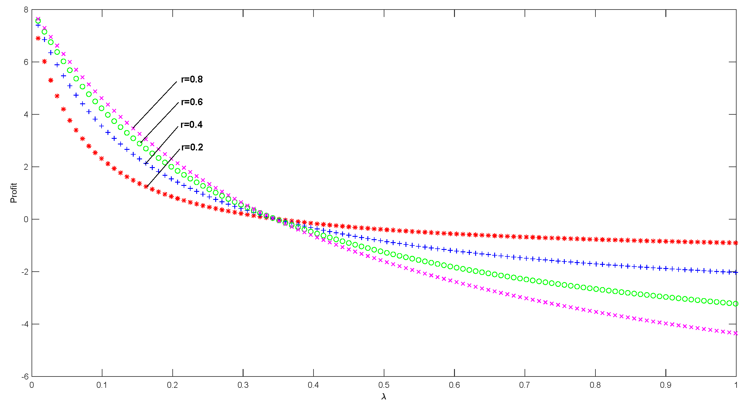
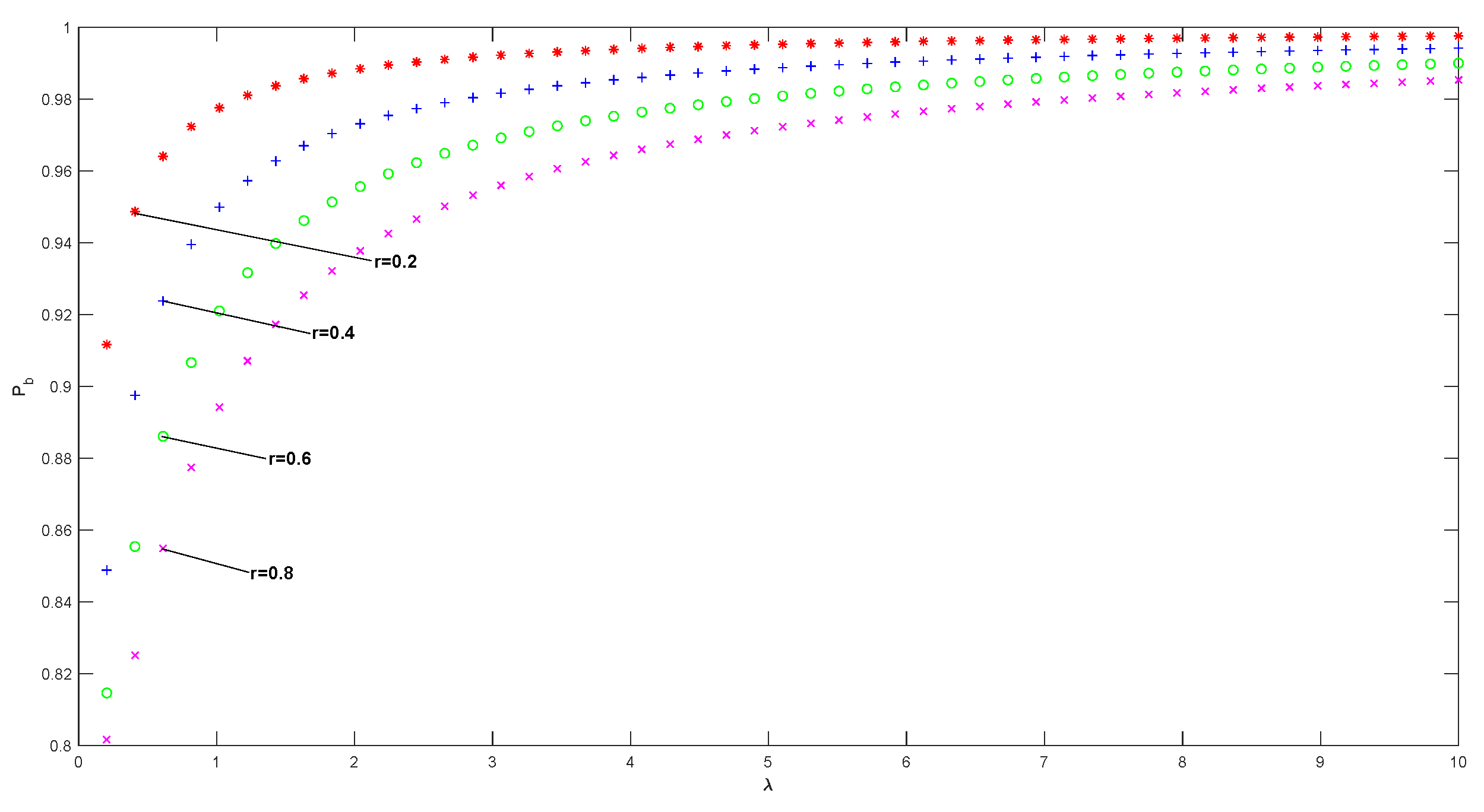
5. Availability Analysis Based on Numerical Simulation

In this section, several numerical examples are presented to elucidate the results obtained in the preceding Section 4.1.

Let $T_p$ denote the total profit of the five-robot system equipped with warning functions. Thus, we have the following formula for calculating benefits, namely

$$\begin{array}{c}\hfill T_p=I_1{A}_s-W_1{F}_{sf},\end{array}$$

where $I_1$ and $W_1$ denote the revenue generated by the five-robot system equipped with warning functions per unit time and the loss incurred due to faulty components, respectively.

(1) Let $\lambda ={\lambda }_s=\alpha ={\lambda }_{hi}(i=0,1,2,3,4)$ and $r=r_E=r_5\left(x\right)=r_6\left(x\right)$.

Table 1. Availability analysis.

$\mathit{\lambda }$	${\mathit{A}}_{\mathit{s}0.1}$	${\mathit{A}}_{\mathit{s}0.2}$	${\mathit{A}}_{\mathit{s}0.3}$	${\mathit{A}}_{\mathit{s}0.4}$	${\mathit{A}}_{\mathit{s}0.5}$	${\mathit{A}}_{\mathit{s}0.6}$	${\mathit{A}}_{\mathit{s}0.7}$	${\mathit{A}}_{\mathit{s}0.8}$	${\mathit{A}}_{\mathit{s}0.9}$
0.1	0.079	0.244	0.403	0.529	0.622	0.690	0.741	0.780	0.809
0.2	0.041	0.137	0.250	0.357	0.449	0.525	0.587	0.637	0.678
0.3	0.028	0.095	0.181	0.269	0.350	0.422	0.485	0.538	0.583
0.4	0.021	0.073	0.141	0.215	0.287	0.353	0.412	0.465	0.511
0.5	0.017	0.059	0.116	0.179	0.243	0.303	0.359	0.409	0.454
0.6	0.014	0.050	0.099	0.154	0.210	0.266	0.317	0.365	0.409
0.7	0.012	0.043	0.086	0.135	0.186	0.236	0.285	0.330	0.372
0.8	0.010	0.038	0.076	0.120	0.166	0.213	0.258	0.301	0.341
0.9	0.009	0.030	0.061	0.098	0.137	0.177	0.217	0.256	0.292

presents nine distinct failure rate scenarios, where $A_{sr}$ denotes system availability at $r=0.1$, $0.2$, $0.3$, $0.4$, $0.5$, $0.6$, $0.7$, $0.8$, $0.9$. The data indicate that, when the total repair rate r is constant, the availability $A_{sr}$ gradually decreases as the failure rate $\lambda$ increases. Conversely, system availability improves as the repair rate increases.

Figure 4 illustrates the steady-state availability of the system with fixed parameter values $\lambda ={\lambda }_s=\alpha ={\lambda }_{hi}(i=0,1,2,3,4)$ and $r=r_E=r_5\left(x\right)=r_6\left(x\right)=0.2,0.4,0.6,0.8$.

(2) According to Equation (71), let $\lambda ={\lambda }_s=\alpha ={\lambda }_{hi}(i=0,1,2,3,4)$ and $r=r_E=r_5\left(x\right)=r_6\left(x\right)$.

Table 2. Fault frequency analysis.

$\mathit{\lambda }$	${\mathit{F}}_{\mathit{s}0.1}$	${\mathit{F}}_{\mathit{s}0.2}$	${\mathit{F}}_{\mathit{s}0.3}$	${\mathit{F}}_{\mathit{s}0.4}$	${\mathit{F}}_{\mathit{s}0.5}$	${\mathit{F}}_{\mathit{s}0.6}$	${\mathit{F}}_{\mathit{s}0.7}$	${\mathit{F}}_{\mathit{s}0.8}$	${\mathit{F}}_{\mathit{s}0.9}$
0.1	0.046	0.141	0.234	0.308	0.363	0.403	0.432	0.454	0.471
0.2	0.047	0.157	0.288	0.412	0.520	0.609	0.682	0.742	0.790
0.3	0.047	0.163	0.311	0.463	0.605	0.732	0.841	0.935	1.015
0.4	0.047	0.166	0.323	0.493	0.659	0.813	0.951	1.074	1.182
0.5	0.047	0.168	0.331	0.513	0.696	0.870	1.032	1.179	1.311
0.6	0.047	0.169	0.337	0.527	0.722	0.913	1.093	1.260	1.413
0.7	0.047	0.170	0.341	0.537	0.743	0.946	1.142	1.326	1.496
0.8	0.047	0.171	0.344	0.545	0.759	0.973	1.181	1.379	1.565
0.9	0.047	0.171	0.347	0.552	0.771	0.994	1.213	1.424	1.624

presents nine distinct cases of repair rates, where $F_{sfr}$ denotes the system failure frequency for $r=0.1,0.2,0.3,0.4,0.5,0.6,0.7,0.8,0.9$. According to the data, when the total repair rate r is fixed, the failure frequency $F_{sfr}$ gradually increases as the failure rate $\lambda$ rises. Consequently, as the repair rate increases, the system’s performance improves.

Figure 5 illustrates the steady-state failure frequency of the system with fixed parameter values $\lambda ={\lambda }_s=\alpha ={\lambda }_{hi}(i=0,1,2,3,4)$ and $r=r_E=r_5\left(x\right)=r_6\left(x\right)=0.2,0.4,0.6,0.8$.

(3) Let $\lambda ={\lambda }_s=\alpha ={\lambda }_{hi}(i=0,1,2,3,4)$ and $r=r_E=r_5\left(x\right)=r_6\left(x\right),I_1=8,W_1=4$.

Table 3. Profit analysis.

$\mathit{\lambda }$	${\mathit{T}}_{\mathit{p}0.1}$	${\mathit{T}}_{\mathit{p}0.2}$	${\mathit{T}}_{\mathit{p}0.3}$	${\mathit{T}}_{\mathit{p}0.4}$	${\mathit{T}}_{\mathit{p}0.5}$	${\mathit{T}}_{\mathit{p}0.6}$	${\mathit{T}}_{\mathit{p}0.7}$	${\mathit{T}}_{\mathit{p}0.8}$	${\mathit{T}}_{\mathit{p}0.9}$
0.1	0.45	1.39	2.29	3.00	3.53	3.91	4.20	4.42	4.59
0.2	0.14	0.47	0.85	1.21	1.51	1.76	1.96	2.13	2.27
0.3	0.03	0.11	0.20	0.30	0.38	0.45	0.51	0.56	0.60
0.4	−0.02	−0.08	−0.16	−0.25	−0.34	−0.43	−0.51	−0.58	−0.64
0.5	−0.06	−0.20	−0.40	−0.62	−0.84	−1.06	−1.26	−1.44	−1.61
0.6	−0.08	−0.28	−0.56	−0.88	−1.21	−1.53	−1.83	−2.12	−2.38
0.7	−0.09	−0.34	−0.68	−1.07	−1.49	−1.90	−2.29	−2.66	−3.01
0.8	−0.11	−0.38	−0.77	−1.22	−1.71	−2.19	−2.66	−3.11	−3.53
0.9	−0.12	−0.42	−0.84	−1.35	−1.88	−2.43	−2.97	−3.48	−3.98

presents nine distinct cases of failure rates, where $T_{pr}$ denotes the system profit for $r=0.1,0.2,0.3,0.4,0.5,0.6,0.7,0.8,0.9$. According to the data, (I) as the failure rate $\lambda$ increases, the system profit $T_{pr}$ gradually decreases. (II) As the repair rate r increases, the system profit $T_{pr}$ gradually increases. Therefore, it can be concluded that a system equipped with early warning functions can mitigate losses and enhance profits.

Figure 6 illustrates the system profit with fixed parameter values $I_1=8,W_1=4,\lambda ={\lambda }_s=\alpha ={\lambda }_{hi}(i=0,1,2,3,4)$, and $r=r_E=r_5\left(x\right)=r_6\left(x\right)=0.2,0.4,0.6,0.8$.

(4) According to Equation (72), let $\lambda ={\lambda }_s=\alpha ={\lambda }_{hi}(i=0,1,2,3,4),r=r_E=r_5\left(x\right)=r_6\left(x\right)$.

Table 4. Analysis of repair equipment being busy.

$\mathit{\lambda }$	${\mathit{P}}_{\mathit{b}0.1}$	${\mathit{P}}_{\mathit{b}0.2}$	${\mathit{P}}_{\mathit{b}0.3}$	${\mathit{P}}_{\mathit{b}0.4}$	${\mathit{P}}_{\mathit{b}0.5}$	${\mathit{P}}_{\mathit{b}0.6}$	${\mathit{P}}_{\mathit{b}0.7}$	${\mathit{P}}_{\mathit{b}0.8}$	${\mathit{P}}_{\mathit{b}0.9}$
0.1	0.971	0.915	0.867	0.839	0.826	0.826	0.832	0.844	0.859
0.2	0.985	0.950	0.910	0.875	0.848	0.828	0.814	0.806	0.802
0.3	0.990	0.965	0.934	0.903	0.875	0.852	0.834	0.819	0.808
0.4	0.992	0.973	0.948	0.921	0.896	0.873	0.854	0.837	0.824
0.5	0.994	0.978	0.957	0.934	0.911	0.890	0.871	0.854	0.839
0.6	0.995	0.982	0.963	0.943	0.923	0.903	0.885	0.868	0.853
0.7	0.996	0.984	0.968	0.950	0.931	0.913	0.896	0.880	0.865
0.8	0.996	0.986	0.972	0.956	0.939	0.922	0.905	0.890	0.876
0.9	0.997	0.987	0.975	0.960	0.944	0.928	0.913	0.899	0.885

presents nine distinct cases of failure rates, where $P_{br}$ denotes the probability of the repair equipment being occupied for $r=0.1,0.2,0.3,0.4,0.5,0.6,0.7,0.8,0.9$. The data indicate that when the total repair rate r is fixed, the probability $P_{br}$ of the repair equipment being busy increases progressively as the failure rate $\lambda$ rises. Consequently, as the failure rate increases, the repair equipment becomes increasingly occupied.

Figure 7 illustrates the status of the repair equipment being occupied in the system when the parameter values are fixed at $\lambda ={\lambda }_s=\alpha ={\lambda }_{hi}(i=0,1,2,3,4),r=r_E=r_5\left(x\right)=r_6\left(x\right)=0.2,0.4,0.6,0.8$.

6. Conclusions

A mathematical model of a five-robot system with early warning functionality has been established using the supplementary variable method, employing pure analytical techniques and semigroup theory to verify the existence and uniqueness of the system solution. Utilizing cofinal correlation theory, spectral analysis methods, and $C_0$-semigroup theory, the properties of the system’s main operator and its spectral distribution are presented. Furthermore, the asymptotic stability of the system’s solution is verified. The primary reliability indicators of the system are derived using the eigenvector method associated with the zero eigenvalue. The analytical and numerical solutions of the five-robot system with early warning functions were presented. A availability analysis based on numerical simulations was presented. As anticipated, the findings presented in this paper are enhanced by the probabilistic analysis method. Consequently, the novel approach introduced in this paper addresses the challenges associated with studying time-varying solutions and varying system parameters. Firstly, the innovation of this paper lies in the combination of qualitative and quantitative analyses to improve and enrich the theory and methods of repairable systems. Secondly, in the early warning system, when the alarm indicates a false alert, the model of the robotic system with early warning functions approaches that of a repairable system without early warning functions. Further research should be conducted on the relationship between early warning systems and non-early warning systems, and the connections between their steady-state solutions should be explored. In the future, we aspire to develop more practical complex systems, thereby enabling the methods proposed in this paper to be applied to multi-state repairable systems.

References

1. Dhillon, B.S.; AnudeIncome, O.C. Optimization of a repairable and redundant system. Microelectron. Reliab. 1994, 34, 1709–1720. [Google Scholar] [CrossRef]
2. Yang, N.; Dhillon, B.S. Stochastic analysis of a general standby system with constant human error and arbitrarily system repair rates. Microelectron. Reliab. 1995, 35, 1037–1045. [Google Scholar] [CrossRef]
3. Liu, H.; Wang, Y.; Ji, W.; Wang, L. A Context-Aware Safety System for Human-Robot Collaboration. Procedia Manuf. 2018, 17, 238–245. [Google Scholar] [CrossRef]
4. Zheng, K.; Hu, Y.; Wu, B. Intelligent fuzzy sliding mode control for complex robot system with disturbances. Eur. J. Control 2020, 51, 95–109. [Google Scholar] [CrossRef]
5. Ajoudani, A.; Zanchettin, A.M.; Ivaldi, S.; Albu-Schäffer, A.; Kosuge, K.; Khatib, O. Progress and prospects of the human-robot collaboration. Auton. Robot. 2018, 42, 957–975. [Google Scholar] [CrossRef]
6. Leite, A.; Pinto, A.; Matos, A. A safety monitoring model for a faulty mobile robot. Robotics 2018, 7, 32. [Google Scholar] [CrossRef]
7. Huang, Y.; Xiang, X.; Zhou, H.; Yan, C.; Chang, Y.; Sun, Y. Multi-robot self-organizing cooperative pursuit method based on probabilistic graphical model. Control. Theory Appl. 2023, 40, 2225–2235. [Google Scholar]
8. Reza, G.; Mehdi, M.F. Robust Control of Robotic Manipulators in the Task-Space Using an Adaptive Observer Based on Chebyshev Polynomials. J. Syst. Sci. Complex. 2020, 33, 1360–1382. [Google Scholar]
9. Qiao, X.; Ma, D.; Yao, X.; Feng, B. Stability and Numerical Analysis of a Standby System. J. Shanghai Jiaotong Univ. Sci. 2020, 25, 769–778. [Google Scholar] [CrossRef]
10. Gerasimos, R. A Nonlinear Optimal Control Approach for Tracked Mobile Robots. J. Syst. Sci. Complex. 2021, 34, 1279–1300. [Google Scholar]
11. Wang, S.; Lu, S. Dynamic Optimization of Robot Automatic Control System Based on Differential Algebraic Equations. Appl. Math. Nonlinear Sci. 2023, 8, 3149–3158. [Google Scholar] [CrossRef]
12. Jiang, H.; Yang, F. Application of industrial robot based on infrared sensor technology in monitoring of electrical equipment. Appl. Math. Nonlinear Sci. 2024, 9, 1–16. [Google Scholar] [CrossRef]
13. Ke, X.; Liu, S. Exponential Stability of Impulsive Neutral Stochastic Functional Differential Equations with Markovian Switching. J. Syst. Sci. Complex. 2023, 36, 1560–1582. [Google Scholar]
14. Jain, M.; Rakhee; Singh, M. Bilevel control of degraded machining system with warm standbys, setup and vacation. Appl. Math. Model. 2004, 28, 1015–1026. [Google Scholar] [CrossRef]
15. Ke, J.C.; Wang, K.H. Vacation policies for machine repair problem with two type spares. Appl. Math. Model. 2007, 31, 880–894. [Google Scholar] [CrossRef]
16. Gaver, D.P. Time to failure and availability of paralleled systems with repair. IEEE Trans. Reliab. 1963, 12, 30–38. [Google Scholar] [CrossRef]
17. Pazy, A. Semigroups of Linear Operators and Applications to Partial Differential Equations; Springer Science Business Media: Berlin/Heidelberg, Germany, 2012. [Google Scholar]
18. Gurtin, M.E.; MacCamy, R.C. Non-linear age-dependent population dynamics. Arch. Ration. Mech. Anal. 1974, 54, 281–300. [Google Scholar] [CrossRef]
19. Dunford, N.; Schwartz, J.T. Linear Operators Part I: General Theory; Interscience Publishers: New York, NY, USA, 1958. [Google Scholar]
20. Arendt, W. Resolvent positive operators. Proc. Lond. Math. Soc. 1987, 3, 321–349. [Google Scholar] [CrossRef]
21. Zhang, X. Reliability analysis of a cold standby repairable system with repairman extra work. J. Syst. Sci. Complex. 2015, 28, 1015–1032. [Google Scholar] [CrossRef]
22. Wang, Y.; Qiao, X.; Zhan, B.; Ma, D.; Zhao, G. The Stability and Reliability Analysis of a System Containing Two Redundant Robots. In Proceedings of the 2014 Sixth International Conference on Intelligent Human-Machine Systems and Cybernetics, Hangzhou, China, 26–27 August 2014; Volume 1, pp. 288–291. [Google Scholar]
23. Yuan, W.; Xu, G. Spectral analysis of a two unit deteriorating standby system with repair. WSEAS Trans. Math. 2011, 10, 125–138. [Google Scholar]
24. Taylor, A.E.; Lay, D.C. Introduction to Functional Analysis; Wiley: New York, NY, USA, 1958. [Google Scholar]
25. Arendt, W.; Grabosch, A.; Greiner, G.; Moustakas, U.; Nagel, R.; Schlotterbeck, U.; Groh, U.; Lotz, H.P.; Neubrander, F. One-Parameter Semigroups of Positive Operators; Springer: Berlin/Heidelberg, Germany, 2006. [Google Scholar]
26. MATLAB. 9.6.0.1.1072779. MathWorks. March 2019. Available online: https://ww2.mathworks.cn/products/matlab.html (accessed on 12 March 2019).
Figure 1. System state-transition diagram.
Axioms 14 00113 g001
Figure 2. Numerical solution of the five-robot system (74)–(81), (a) p 0 ( t ) with ζ = 0.1 , and ζ = 0.3 , (b) p 1 ( t ) with ζ = 0.1 , and ζ = 0.3 , (c) p 2 ( t ) with ζ = 0.1 , and ζ = 0.3 , (d) p 3 ( t ) with ζ = 0.1 , and ζ = 0.3 .
Axioms 14 00113 g002aAxioms 14 00113 g002b
Figure 3. Numerical solution of the five-robot system (74)–(81), (a) p 4 ( t ) with ζ = 0.1 , and ζ = 0.3 , (b) p E ( t ) with ζ = 0.1 , and ζ = 0.3 , (c) p 5 ( t ) with ζ = 0.1 , and ζ = 0.3 , (d) p 6 ( t ) with ζ = 0.1 , and ζ = 0.3 .
Axioms 14 00113 g003aAxioms 14 00113 g003b
Figure 4. Availability of system.
Axioms 14 00113 g004
Figure 5. Fault frequency.
Axioms 14 00113 g005
Figure 6. Profit of system.
Axioms 14 00113 g006
Figure 7. Probability of repair equipment being busy.
Axioms 14 00113 g007