Article

Spherical Fuzzy Credibility Dombi Aggregation Operators and Their Application in Artificial Intelligence

1
Department of Mathematics, Abdul Wali Khan University Mardan, Mardan 23200, Pakistan
2
Department of Mathematics, Riphah International University Faisalabad Campus, Faisalabad 38000, Pakistan
3
Department of Mathematics, Saveetha School of Engineering, Saveetha Institute of Medical and Technical Sciences, Saveetha University, Chennai 602105, Tamil Nadu, India
4
College of Global Business, Korea University, Sejong 30019, Republic of Korea
5
Faculty of Applied Management, Economics, and Finance, University Business Academy in Novi Sad, Jevrejska 24, 11000 Belgrade, Serbia
6
Faculty of Information Technologies, Pan-European University "APEIRON", Vojvode Pere Krece 13, 78102 Banja Luka, Bosnia and Herzegovina
7
Technical Faculty in Bor, University of Belgrade, Vojske Jugoslavije 12, 19210 Bor, Serbia
*
Author to whom correspondence should be addressed.
Axioms 2025, 14(2), 108; https://doi.org/10.3390/axioms14020108
Submission received: 12 January 2025 / Revised: 24 January 2025 / Accepted: 29 January 2025 / Published: 31 January 2025
(This article belongs to the Special Issue New Perspectives in Fuzzy Sets and Their Applications, 2nd Edition)

Abstract

:
It was recently proposed to extend the spherical fuzzy set to spherical fuzzy credibility sets (SFCSs). In this paper, we define the concept of SFCSs. We then define new operational laws for SFCSs using Dombi operational laws. Various spherical fuzzy credibility aggregation operators such as spherical fuzzy credibility Dombi weighted averaging (SFCDWA), spherical fuzzy credibility Dombi ordered weighted averaging (SFCDOWA), spherical fuzzy credibility Dombi weighted geometric (SFCDWG), and spherical fuzzy credibility Dombi ordered weighted geometric (SFCDOWG) are defined. We also show the boundedness, monotonicity, and idempotency aspects of the suggested operators. We proposed the spherical fuzzy credibility entropy to find the unknown weight information of the attributes. Symmetry analysis is a useful and important tool in artificial intelligence that may be used in a variety of fields. To calculate the significant factor, we determine the multi-attribute decision-making (MADM) method using the suggested operators for SFCSs to increase the value of the assessed operators. To demonstrate the effectiveness and superiority of the suggested approach, we compare our findings to those of many other approaches.

1. Introduction

In everyday life, system complexity is increasing; as a result, executives and decision makers are having difficulty selecting the optimal option from a group of alternatives. Many organizations had difficulty defining motivated goals and removing opinion issues. Obtaining a single objective to summarize is tough, but not impossible. Different businesses have a variety of goals and face numerous uncertainties, ambiguities, and ambiguity in facts regarding the solution of practical problems, limiting decision makers’ ability to obtain a reliable and appropriate technique for determining the best alternative.
In artificial intelligence, symmetry analysis [1] is a multifaceted approach that includes data manipulation, algorithm design, knowledge representation, and fairness selections [2]. Artificial intelligence may be made more capable, equitable, dominant, and comprehensible in a variety of fields by employing symmetry analysis techniques. These ideas have also been used in a wide range of domains, including artificial intelligence, game theory, machine learning, neural networks, data mining, and decision making while taking into account traditional set theory [3]. Unfortunately, because there are only two options—zero and one—these techniques have resulted in losing a great deal of information. To retain more information, a stronger notion is therefore needed. Zadeh [4] created a fuzzy set (FS) in which the truth grade μ y ^ ( 𝖥 u ¯ ) of an FS becomes μ y ^ ( 𝖥 u ¯ ) [ 0 , 1 ] . Zhang et al. [5] defined the concept of a fuzzy control model and simulation for nonlinear supply chain systems with lead times. Zhang et al. [6] proposed a discrete switched model and fuzzy robust control of a dynamic supply chain network. Sarwar and Li [7] developed fuzzy fixed point results and applications to ordinary fuzzy differential equations in complex valued metric spaces. Gao et al. [8] suggested SMC for semi-Markov jump TS fuzzy systems with time delay. Xia et al. [9] presented further results on fuzzy sampled-data stabilization of chaotic nonlinear systems. Also, a variety of disciplines have utilized this FS idea [10,11,12,13]. Moreover, Atanassov [14] introduced the concept of intuitionistic FS (IFS) by modifying the FS theory by adding another grade of falsehood ν y ^ ( 𝖥 u ¯ ) with the condition that 0 μ y ^ ( 𝖥 u ¯ ) + ν y ^ ( 𝖥 u ¯ ) 1 , and a variety of disciplines have utilized this IFS idea [15,16,17,18,19,20]. However, the concept of IFS has not been particularly effective when the pair ( 0.6 , 0.5 ) is present. Yager [21], therefore, introduced the Pythagorean fuzzy sets (PyFSs) with the additional requirement that 0 μ y ^ 2 ( 𝖥 u ¯ ) + ν y ^ 2 ( 𝖥 u ¯ ) 1 ; consequently, various programs use PyFS [22,23,24]. In spite of this, the PyFS’s restricted characteristics cause it to still fail when the pair (0.9, 0.8) exists. Therefore, the concept of q-rung orthopair FSs (q-ROFSs) was then introduced by Yager [25], with the dominating and notable condition 0 μ y ^ Q s ( 𝖥 u ¯ ) + ν y ^ Q S ( 𝖥 u ¯ ) 1 , Q S 1 . Numerous fields have utilized these q-ROFSs [26,27,28]. Coung [29] developed picture fuzzy sets (PFSs), which consist of three kinds of responses: truth μ y ^ ( 𝖥 u ¯ ) , abstention ν y ^ ( 𝖥 u ¯ ) , and falsity η y ^ ( 𝖥 u ¯ ) grades to handle incompatibilities in data with the condition that 0 μ y ^ ( 𝖥 u ¯ ) + ν y ^ ( 𝖥 u ¯ ) + η y ^ ( 𝖥 u ¯ ) 1 . These PFSs have been applied in many areas [30,31,32]. However, PFS encounters difficulties when presented with numbers whose total exceeds the unit interval. To address this, Mahmood [33] introduced spherical fuzzy sets (SFS), modifying the PFS with the condition that 0 μ y ^ 2 ( 𝖥 u ¯ ) + ν y ^ 2 ( 𝖥 u ¯ ) + η y ^ 2 ( 𝖥 u ¯ ) 1 . These SFSs have been applied in many areas [34,35,36]. Ye [37] thoroughly demonstrated a new idea recognized as the fuzzy credibility set (FCS). The fuzzy credibility sets (FCSs) have been applied in many areas [38,39,40]. Furthermore, Qiyas [41] developed intuitionistic fuzzy credibility number. The Dombi t-norm (DTN) and the Dombi t-conorm (DTCN) are the names given to the original concepts of t-norm and t-conorm, which were introduced by Dombi [42] in 1982. several researchers have deduced several types of operators based on DTN and DTCN. Based on PFSs, Khan et al. [43] provided the Dombi operators. The Dombi operators for q-ROFSs and their applications were first introduced by Jana et al. [44]. Dombi aggregation operators (AOs) for q-ROFSs were assessed by Du [45]. Dombi operators were analyzed by Seikh and Mandal [46] for IFSs.
In this paper, we advance the study of SFCNs with Dombi averaging and geometric operators. During the aggregation process, the most important process is to define the operational laws. In this manner, with the developing sound of the SFCS both inside and out of scope, there is a need to build up some new operational laws and aggregation operators. By keeping the benefits of SFCS, we characterize aggregation operators of SFCSs. In addition to this, in the field of the aggregation process, the most fundamental weighted average and geometric operators by utilizing Dombi norms have been characterized.
The objective of this study are the following:
  • In this paper, a new notion, spherical fuzzy credibility numbers (SFCNs), based on mixed information including spherical fuzzy values and its credibility value, is presented. This new idea promotes the rationality and validity of data.
  • Using Dombi operation laws, we define new operation laws for spherical fuzzy credibility numbers.
  • Based on the defined operation laws, some averaging and geometric aggregation operators are defined.
  • With the help of the SFCDWA and SFCDWG operators that are built into SFCNs, together with their operational laws and score functions, one may use SFCN data to solve MADM issues with the useful mathematical tools.
  • Using specified operators, a numerical example is solved.
  • The research paper examines the benefits of the suggested data, emphasizing the discovered operators’ representations and the mathematical tool.
  • A comparative examination of the proposed data is undertaken by contrasting them with certain pre-existing methods.
The paper’s sections are listed and organized as follows: In Section 2, the definitions of SFCNs are reviewed along with certain required notions and a new definition that is extended. We present the operating guidelines for SFCNs based on DTN and DTCN in Section 3. We also use these operational principles to define new aggregation operators. SFC MADM difficulties are tackled in a new way in Section 4 by employing SFCDWA and SFCDWG operators. We used the MADM technique and the discovered operators in Section. In Section 5, delves deeply into how the parameters affect the outcomes of decision making. In Section 6, a comparison of the proposed data with the available ones is shown in Section 7. Finally, the conclusion is shown in Section 7.

2. Preliminaries

Definition 1
([4]). Let U ¯ 0 . Let Ξ be a fuzzy set that is deduced from U ¯ defined as
Ξ = { ( 𝖥 u ¯ , μ y ^ ( 𝖥 u ¯ ) ) | 𝖥 u ¯ U ¯ } ,
and the fuzzy set Ξ’s member is represented as μ y ^ ( 𝖥 u ¯ ) : U ¯ [ 0 , 1 ] .
Definition 2
([14]). Let U ¯ 0 . Let Ξ be a instuitionistic fuzzy set (IFS) that is deduced from U ¯ defined as
Ξ = 𝖥 u ¯ , μ y ^ ( 𝖥 u ¯ ) , ν y ^ ( 𝖥 u ¯ ) | 𝖥 u ¯ U ¯ ,
here μ y ^ ( 𝖥 u ¯ ) , ν y ^ ( 𝖥 u ¯ ) : U ¯ [ 0 , 1 ] are membership degree (MD) and nom-membership degree (NMD) functions and an IFN is represented as μ y ^ ( 𝖥 u ¯ ) , ν y ^ ( 𝖥 u ¯ ) such that 0 μ y ^ ( 𝖥 u ¯ ) + ν y ^ ( 𝖥 u ¯ ) 1 and π y ^ ( 𝖥 u ¯ ) : U ¯ 0 , 1 is the degree of hesitancy and π y ^ ( 𝖥 u ¯ ) = 1 μ y ^ ( 𝖥 u ¯ ) ν y ^ ( 𝖥 u ¯ ) .
Definition 3
([21]). Let U ¯ 0 . Let Ξ be a Pythagorean fuzzy set (PyFS) that is deduced from U ¯ defined as
Ξ = 𝖥 u ¯ , μ y ^ ( 𝖥 u ¯ ) , ν y ^ ( 𝖥 u ¯ ) | 𝖥 u ¯ U ¯ ,
here μ y ^ ( 𝖥 u ¯ ) , ν y ^ ( 𝖥 u ¯ ) : U ¯ [ 0 , 1 ] are MD and NMD functions and a PyFN is represented as μ y ^ ( 𝖥 u ¯ ) , ν y ^ ( 𝖥 u ¯ ) such that, 0 μ y ^ 2 ( 𝖥 u ¯ ) + ν y ^ 2 ( 𝖥 u ¯ ) 1 , 𝖥 u ¯ U ¯ and π y ^ ( 𝖥 u ¯ ) : U ¯ 0 , 1 is the degree of hesitancy and is defined as π y ^ ( 𝖥 u ¯ ) = 1 μ y ^ 2 ( 𝖥 u ¯ ) ν y ^ 2 ( 𝖥 u ¯ ) .
Definition 4
([29]). Let U ¯ 0 . Let Ξ be a picture fuzzy set (PFS) that is deduced from U ¯ defined as
Ξ = 𝖥 u ¯ , μ y ^ ( 𝖥 u ¯ ) , ν y ^ ( 𝖥 u ¯ ) , η y ^ ( 𝖥 u ¯ ) | 𝖥 u ¯ U ¯ ,
here μ y ^ ( 𝖥 u ¯ ) , ν y ^ ( 𝖥 u ¯ ) , η y ^ ( 𝖥 u ¯ ) : U ¯ [ 0 , 1 ] are MD, neutral membership degree (NuMD), and NMD functions and a PFN is represented as μ y ^ ( 𝖥 u ¯ ) , ν y ^ ( 𝖥 u ¯ ) , η y ^ ( 𝖥 u ¯ ) such that 0 μ y ^ ( 𝖥 u ¯ ) + ν y ^ ( 𝖥 u ¯ ) + η y ^ ( 𝖥 u ¯ ) 1 , 𝖥 u ¯ U ¯ and π y ^ ( 𝖥 u ¯ ) : U ¯ 0 , 1 is the degree of hesitancy and π y ^ ( 𝖥 u ¯ ) = 1 μ y ^ ( 𝖥 u ¯ ) ν y ^ ( 𝖥 u ¯ ) η y ^ ( 𝖥 u ¯ ) .
Definition 5
([33]). Let U ¯ 0 . Let Ξ be a spherical fuzzy set (SFS) that is deduced from U ¯ defined as
Ξ = 𝖥 u ¯ , μ y ^ ( 𝖥 u ¯ ) , ν y ^ ( 𝖥 u ¯ ) , η y ^ ( 𝖥 u ¯ ) | 𝖥 u ¯ U ¯ ,
here μ y ^ ( 𝖥 u ¯ ) , ν y ^ ( 𝖥 u ¯ ) , η y ^ ( 𝖥 u ¯ ) : U ¯ [ 0 , 1 ] are MD, NuMD, and NMD functions and a SFN is represented as μ y ^ ( 𝖥 u ¯ ) , ν y ^ ( 𝖥 u ¯ ) , η y ^ ( 𝖥 u ¯ ) such that 0 μ y ^ 2 ( 𝖥 u ¯ ) + ν y ^ 2 ( 𝖥 u ¯ ) + η y ^ 2 ( 𝖥 u ¯ ) 1 , 𝖥 u ¯ U ¯ and π y ^ ( 𝖥 u ¯ ) : U ¯ 0 , 1 is the degree of hesitancy of and π y ^ ( 𝖥 u ¯ ) = 1 μ y ^ 2 ( 𝖥 u ¯ ) ν y ^ 2 ( 𝖥 u ¯ ) η y ^ 2 ( 𝖥 u ¯ ) .
Definition 6
([37]). Let U ¯ 0 . Let Ξ be a fuzzy credibility set that is deduced from U ¯ defined as
Ξ = 𝖥 u ¯ , t y ^ ( 𝖥 u ¯ ) , c y ^ ( 𝖥 u ¯ ) | 𝖥 u ¯ U ¯ ,
here t y ^ ( 𝖥 u ¯ ) , c y ^ ( 𝖥 u ¯ ) : U ¯ [ 0 , 1 ] are functions where t y ^ ( 𝖥 u ¯ ) is the MD and c y ^ ( 𝖥 u ¯ ) is the degree of credibility linked t y ^ ( 𝖥 u ¯ ) , and fuzzy credibility number is represented as t y ^ ( 𝖥 u ¯ ) , c y ^ ( 𝖥 u ¯ ) .
Definition 7
([41]). Let U ¯ 0 . Let Ξ be an intuitionistic fuzzy credibility number (IFCN) that is deduced from U ¯ and defined as
Ξ = 𝖥 u ¯ , t y ^ ( 𝖥 u ¯ ) , c y ^ ( 𝖥 u ¯ ) , r y ^ ( 𝖥 u ¯ ) , d y ^ ( 𝖥 u ¯ ) | 𝖥 u ¯ U ¯ ,
here t y ^ ( 𝖥 u ¯ ) , r y ^ ( 𝖥 u ¯ ) : U ¯ [ 0 , 1 ] are MD and NMD functions. Additionally, c y ^ ( 𝖥 u ¯ ) , d y ^ ( 𝖥 u ¯ ) : U ¯ [ 0 , 1 ] are functions, signifying the degree of credibility linked to t y ^ ( 𝖥 u ¯ ) , r y ^ ( 𝖥 u ¯ ) , respectively, and intuitionistic fuzzy credibility number is represented as t y ^ ( 𝖥 u ¯ ) , c y ^ ( 𝖥 u ¯ ) , r y ^ ( 𝖥 u ¯ ) , d y ^ ( 𝖥 u ¯ ) and fulfills these conditions 0 t y ^ ( 𝖥 u ¯ ) + c y ^ ( 𝖥 u ¯ ) 1 , 0 r y ^ ( 𝖥 u ¯ ) + d y ^ ( 𝖥 u ¯ ) 1 .
Definition 8.
Let U ¯ 0 . Let Ξ be a spherical fuzzy credibility number (SFCN) that is deduced from U ¯ and defined as
Ξ = 𝖥 u ¯ , j y ^ ( 𝖥 u ¯ ) , m y ^ ( 𝖥 u ¯ ) , k y ^ ( 𝖥 u ¯ ) , n y ^ ( 𝖥 u ¯ ) , l y ^ ( 𝖥 u ¯ ) , p y ^ ( 𝖥 u ¯ ) | 𝖥 u ¯ G ,
here j y ^ ( 𝖥 u ¯ ) , k y ^ ( 𝖥 u ¯ ) , l y ^ ( 𝖥 u ¯ ) : U ¯ [ 0 , 1 ] are MD, NuMD, and NMD functions. Additionally, m y ^ ( 𝖥 u ¯ ) , n y ^ ( 𝖥 u ¯ ) , p y ^ ( 𝖥 u ¯ ) : U ¯ [ 0 , 1 ] are functions, signifying the degree of credibility linked to j y ^ ( 𝖥 u ¯ ) , k y ^ ( 𝖥 u ¯ ) , l y ^ ( 𝖥 u ¯ ) , respectively, and SFCN is represented as j y ^ ( 𝖥 u ¯ ) , m y ^ ( 𝖥 u ¯ ) , k y ^ ( 𝖥 u ¯ ) , n y ^ ( 𝖥 u ¯ ) , l y ^ ( 𝖥 u ¯ ) , p y ^ ( 𝖥 u ¯ ) and fulfills these conditions 0 j y ^ ( 𝖥 u ¯ ) 2 + m y ^ ( 𝖥 u ¯ ) 2 1 , 0 k y ^ ( 𝖥 u ¯ ) 2 + n y ^ ( 𝖥 u ¯ ) 2 1 , 0 t y ^ ( 𝖥 u ¯ ) 2 + p y ^ ( 𝖥 u ¯ ) 2 1 .
Definition 9.
Let Ξ = j y ^ ( 𝖥 u ¯ ) , m y ^ ( 𝖥 u ¯ ) , k y ^ ( 𝖥 u ¯ ) , n y ^ ( 𝖥 u ¯ ) , l y ^ ( 𝖥 u ¯ ) , p y ^ ( 𝖥 u ¯ ) be an SFCN. Then, a score function is defined as
S c ( Ξ ) = 1 3 j y ^ ( 𝖥 u ¯ ) 2 + m y ^ ( 𝖥 u ¯ ) 2 + k y ^ ( 𝖥 u ¯ ) 2 n y ^ ( 𝖥 u ¯ ) 2 + l y ^ ( 𝖥 u ¯ ) 2 p y ^ ( 𝖥 u ¯ ) 2 .
An accuracy function is defined as
A ( Ξ ) = 1 3 j y ^ ( 𝖥 u ¯ ) 2 + m y ^ ( 𝖥 u ¯ ) 2 + k y ^ ( 𝖥 u ¯ ) 2 + n y ^ ( 𝖥 u ¯ ) 2 + l y ^ ( 𝖥 u ¯ ) 2 + p y ^ ( 𝖥 u ¯ ) 2 .
here S c ( Ξ ) 1 , 1 and A ( Ξ ) belong to 0 , 1 .
Definition 10.
Let Ξ 1 = j y ^ 1 𝖥 u ¯ , m y ^ 1 ( 𝖥 u ¯ ) , k y ^ 1 ( 𝖥 u ¯ ) , n y ^ 1 ( 𝖥 u ¯ ) , l y ^ 1 ( 𝖥 u ¯ ) , p y ^ 1 ( 𝖥 u ¯ ) ,
Ξ 2 = j y ^ 2 ( 𝖥 u ¯ ) , m y ^ 2 ( 𝖥 u ¯ ) , k y ^ 2 ( 𝖥 u ¯ ) , n y ^ 2 ( 𝖥 u ¯ ) , l y ^ 2 ( 𝖥 u ¯ ) , p y ^ 2 ( 𝖥 u ¯ ) be two SCFNs. Then,
1. 
Ξ 1 Ξ 2 , if S c ( Ξ 1 ) S c ( Ξ 2 )
2. 
Ξ 1 Ξ 2 , if S c ( Ξ 1 ) S c ( Ξ 2 )
3. 
If S c ( Ξ 1 ) = S c ( Ξ 2 ) , then
(i). If A ( Ξ 1 ) A ( Ξ 2 ) then Ξ 1 Ξ 2
(ii). If A ( Ξ 1 ) = A ( Ξ 2 ) then Ξ 1 = Ξ 2 .
Definition 11.
Let three spherical fuzzy credibility numbers be
Ξ = j y ^ ( 𝖥 u ¯ ) , m y ^ ( 𝖥 u ¯ ) , k y ^ ( 𝖥 u ¯ ) , n y ^ ( 𝖥 u ¯ ) , l y ^ ( 𝖥 u ¯ ) , p y ^ ( 𝖥 u ¯ ) ,
Ξ 1 = j y ^ 1 ( 𝖥 u ¯ ) , m y ^ 1 ( 𝖥 u ¯ ) , k y ^ 1 ( 𝖥 u ¯ ) , n y ^ 1 ( 𝖥 u ¯ ) , l y ^ 1 ( 𝖥 u ¯ ) , p y ^ 1 ( 𝖥 u ¯ ) ,   Ξ 2 = j y ^ 2 ( 𝖥 u ¯ ) , m y ^ 2 ( 𝖥 u ¯ ) , k y ^ 2 ( 𝖥 u ¯ ) , n y ^ 2 ( 𝖥 u ¯ ) , l y ^ 2 ( 𝖥 u ¯ ) , p y ^ 2 ( 𝖥 u ¯ ) . Then, basic operation is defined as
1. 
p c = l y ^ ( 𝖥 u ¯ ) , p y ^ ( 𝖥 u ¯ ) , k y ^ ( 𝖥 u ¯ ) , n y ^ ( 𝖥 u ¯ ) , j y ^ ( 𝖥 u ¯ ) , m y ^ ( 𝖥 u ¯ ) ;
2. 
Ξ 1 Ξ 2 iff j y ^ 1 ( 𝖥 u ¯ ) j y ^ 2 ( 𝖥 u ¯ ) , m y ^ 1 ( 𝖥 u ¯ ) m y ^ 2 ( 𝖥 u ¯ ) , k y ^ 1 ( 𝖥 u ¯ ) k y ^ 2 ( 𝖥 u ¯ ) ,
n y ^ 1 ( 𝖥 u ¯ ) n y ^ 2 ( 𝖥 u ¯ ) , l y ^ 1 ( 𝖥 u ¯ ) l y ^ 2 ( 𝖥 u ¯ ) , p y ^ 1 ( 𝖥 u ¯ ) p y ^ 2 ( 𝖥 u ¯ ) ;
3. 
Ξ 1 = Ξ 2 iff Ξ 1 Ξ 2 & Ξ 2 Ξ 1 ;
4. 
Ξ 1 Ξ 2 = max ( j y ^ 1 ( 𝖥 u ¯ ) , j y ^ 2 ( 𝖥 u ¯ ) ) , max ( m y ^ 1 ( 𝖥 u ¯ ) , m y ^ 2 ( 𝖥 u ¯ ) ) , min ( k y ^ 1 ( 𝖥 u ¯ ) , k y ^ 2 ( 𝖥 u ¯ ) ) , min ( n y ^ 1 ( 𝖥 u ¯ ) , n y ^ 2 ( 𝖥 u ¯ ) ) , min ( l y ^ 1 ( 𝖥 u ¯ ) , l y ^ 2 ( 𝖥 u ¯ ) ) , min ( p y ^ 1 ( 𝖥 u ¯ ) , p y ^ 2 ( 𝖥 u ¯ ) ) ;
5. 
Ξ 1 Ξ 2 = min ( j y ^ 1 ( 𝖥 u ¯ ) , j y ^ 2 ( 𝖥 u ¯ ) ) , min ( m y ^ 1 ( 𝖥 u ¯ ) , m y ^ 2 ( 𝖥 u ¯ ) ) , min ( k y ^ 1 ( 𝖥 u ¯ ) , k y ^ 2 ( 𝖥 u ¯ ) ) , min ( n y ^ 1 ( 𝖥 u ¯ ) , n y ^ 2 ( 𝖥 u ¯ ) ) , max ( l y ^ 1 ( 𝖥 u ¯ ) , l y ^ 2 ( 𝖥 u ¯ ) ) , max ( p y ^ 1 ( 𝖥 u ¯ ) , p y ^ 2 ( 𝖥 u ¯ ) ) ;
6. 
Ξ 1 Ξ 2 = j y ^ 1 𝖥 u ¯ 2 + j y ^ 2 𝖥 u ¯ 2 j y ^ 1 𝖥 u ¯ 2 j y ^ 2 𝖥 u ¯ 2 , m y ^ 1 𝖥 u ¯ 2 + m y ^ 2 𝖥 u ¯ 2 m y ^ 1 𝖥 u ¯ 2 m y ^ 2 𝖥 u ¯ 2 , k y ^ 1 ( 𝖥 u ¯ ) k y ^ 2 ( 𝖥 u ¯ ) , n y ^ 1 ( 𝖥 u ¯ ) n y ^ 2 ( 𝖥 u ¯ ) , l y ^ 1 ( 𝖥 u ¯ ) l y ^ 2 ( 𝖥 u ¯ ) , p y ^ 1 ( 𝖥 u ¯ ) p y ^ 2 ( 𝖥 u ¯ ) ;
7. 
Ξ 1 Ξ 2 = j y ^ 1 ( 𝖥 u ¯ ) j y ^ 2 ( 𝖥 u ¯ ) , m y ^ 1 ( 𝖥 u ¯ ) m y ^ 2 ( 𝖥 u ¯ ) , k y ^ 1 ( 𝖥 u ¯ ) k y ^ 2 ( 𝖥 u ¯ ) , n y ^ 1 ( 𝖥 u ¯ ) n y ^ 2 ( 𝖥 u ¯ ) , l y ^ 1 𝖥 u ¯ 2 + l y ^ 2 𝖥 u ¯ 2 l y ^ 1 𝖥 u ¯ 2 l y ^ 2 𝖥 u ¯ 2 , p A ¯ 1 𝖥 u ¯ 2 + p y ^ 2 𝖥 u ¯ 2 p y ^ 1 𝖥 u ¯ 2 p y ^ 2 𝖥 u ¯ 2 ;
8. 
φ . Ξ = 1 ( 1 j y ^ ( 𝖥 u ¯ ) 2 ) φ , 1 ( 1 m y ^ ( 𝖥 u ¯ ) 2 ) φ , k y ^ φ ( 𝖥 u ¯ ) , n y ^ φ ( 𝖥 u ¯ ) , l y ^ φ ( 𝖥 u ¯ ) , p y ^ φ ( 𝖥 u ¯ ) ;
9. 
Ξ φ = j y ^ φ ( 𝖥 u ¯ ) , m y ^ φ ( 𝖥 u ¯ ) , k y ^ φ ( 𝖥 u ¯ ) , n y ^ φ ( 𝖥 u ¯ ) , 1 ( 1 l y ^ ( 𝖥 u ¯ ) 2 ) φ , 1 ( 1 p y ^ ( 𝖥 u ¯ ) 2 ) φ .
Definition 12
([42]). For two arbitrary real numbers p , q and α 1 , Dombi operations for real numbers are given by the following:
D o m p , q = 1 1 + 1 p p α + 1 q q α 1 α ;
D o m p , q = 1 1 + p 1 p α + q 1 q α 1 α .
Definition 13.
Let Ξ 1 = j y ^ 1 ( 𝖥 u ¯ ) , m y ^ 1 ( 𝖥 u ¯ ) , k y ^ 1 ( 𝖥 u ¯ ) , n y ^ 1 ( 𝖥 u ¯ ) , l y ^ 1 ( 𝖥 u ¯ ) , p y ^ 1 ( 𝖥 u ¯ ) ,
Ξ 2 = j y ^ 2 ( 𝖥 u ¯ ) , m y ^ 2 ( 𝖥 u ¯ ) , k y ^ 2 ( 𝖥 u ¯ ) , n y ^ 2 ( 𝖥 u ¯ ) , l y ^ 2 ( 𝖥 u ¯ ) , p y ^ 2 ( 𝖥 u ¯ ) be two SFCNs. Then, using DTN and DTCN, the Dombi operations for SFCNs are defined by the following:
  • Ξ 1 Ξ 2 = 1 1 1 + j y ^ 1 ( 𝖥 u ¯ ) 2 1 j y ^ 1 ( 𝖥 u ¯ ) 2 α + j y ^ 2 ( 𝖥 u ¯ ) 2 1 j y ^ 2 ( 𝖥 u ¯ ) 2 α 1 α , 1 1 1 + m y ^ 1 ( 𝖥 u ¯ ) 2 1 m y ^ 1 ( 𝖥 u ¯ ) 2 α + m y ^ 2 ( 𝖥 u ¯ ) 2 1 m y ^ 2 ( 𝖥 u ¯ ) 2 α 1 α , 1 1 + 1 k y ^ 1 ( 𝖥 u ¯ ) k y ^ 1 ( 𝖥 u ¯ ) α + 1 k y ^ 2 ( 𝖥 u ¯ ) k y ^ 2 ( 𝖥 u ¯ ) α 1 α , 1 1 + 1 n y ^ 1 ( 𝖥 u ¯ ) n y ^ 1 ( 𝖥 u ¯ ) α + 1 n y ^ 2 ( 𝖥 u ¯ ) n y ^ 2 ( 𝖥 u ¯ ) α 1 α , 1 1 + 1 l y ^ 1 ( 𝖥 u ¯ ) l y ^ 1 ( 𝖥 u ¯ ) α + 1 l y ^ 2 ( 𝖥 u ¯ ) l y ^ 2 ( 𝖥 u ¯ ) α 1 α , 1 1 + 1 p y ^ 1 ( 𝖥 u ¯ ) p y ^ 1 ( 𝖥 u ¯ ) α + 1 p y ^ 2 ( 𝖥 u ¯ ) p y ^ 2 ( 𝖥 u ¯ ) α 1 α ;
  • Ξ 1 Ξ 2 = 1 1 + 1 j y ^ 1 ( 𝖥 u ¯ ) j y ^ 1 ( 𝖥 u ¯ ) α + 1 j y ^ 2 ( 𝖥 u ¯ ) j y ^ 2 ( 𝖥 u ¯ ) α 1 α , 1 1 + 1 m y ^ 1 ( 𝖥 u ¯ ) m y ^ 1 ( 𝖥 u ¯ ) α + 1 m y ^ 2 ( 𝖥 u ¯ ) m y ^ 2 ( 𝖥 u ¯ ) α 1 α , 1 1 1 + k y ^ 1 ( 𝖥 u ¯ ) 1 k y ^ 1 ( 𝖥 u ¯ ) α + k y ^ 2 ( 𝖥 u ¯ ) 1 k y ^ 2 ( 𝖥 u ¯ ) α 1 α , 1 1 1 + n y ^ 1 ( 𝖥 u ¯ ) 1 n y ^ 1 ( 𝖥 u ¯ ) α + n y ^ 2 ( 𝖥 u ¯ ) 1 n y ^ 2 ( 𝖥 u ¯ ) α 1 α , 1 1 1 + l y ^ 1 ( 𝖥 u ¯ ) 1 l y ^ 1 ( 𝖥 u ¯ ) α + l y ^ 2 ( 𝖥 u ¯ ) 1 l y ^ 2 ( 𝖥 u ¯ ) α 1 α , 1 1 1 + p y ^ 1 ( 𝖥 u ¯ ) 1 p y ^ 1 ( 𝖥 u ¯ ) α + p y ^ 2 ( 𝖥 u ¯ ) 1 p y ^ 2 ( 𝖥 u ¯ ) α 1 α ;
  • φ . Ξ 1 = 1 1 1 + φ . j y ^ 1 ( 𝖥 u ¯ ) 1 j y ^ 1 ( 𝖥 u ¯ ) α 1 α , 1 1 1 + φ . m y ^ 1 ( 𝖥 u ¯ ) 1 m y ^ 1 ( 𝖥 u ¯ ) α 1 α , 1 1 + φ . 1 k y ^ 1 ( 𝖥 u ¯ ) k y ^ 1 ( 𝖥 u ¯ ) α 1 α , 1 1 + φ . 1 n y ^ 1 ( 𝖥 u ¯ ) n y ^ 1 ( 𝖥 u ¯ ) α 1 α , 1 1 + φ . 1 l y ^ 1 ( 𝖥 u ¯ ) l y ^ 1 ( 𝖥 u ¯ ) α 1 α , 1 1 + φ . 1 p y ^ 1 ( 𝖥 u ¯ ) p y ^ 1 ( 𝖥 u ¯ ) α 1 α ;
  • Ξ 1 φ = 1 1 + φ . 1 j y ^ 1 ( 𝖥 u ¯ ) j y ^ 1 ( 𝖥 u ¯ ) α 1 α , 1 1 + φ . 1 m y ^ 1 ( 𝖥 u ¯ ) m y ^ 1 ( 𝖥 u ¯ ) α 1 α , 1 1 1 + φ . k y ^ 1 ( 𝖥 u ¯ ) 1 k y ^ 1 ( 𝖥 u ¯ ) α 1 α , 1 1 1 + φ . n y ^ 1 ( 𝖥 u ¯ ) 1 n y ^ 1 ( 𝖥 u ¯ ) α 1 α , 1 1 1 + φ . l y ^ 1 ( 𝖥 u ¯ ) 1 l y ^ 1 ( 𝖥 u ¯ ) α 1 α , 1 1 1 + φ . p y ^ 1 ( 𝖥 u ¯ ) 1 p y ^ 1 ( 𝖥 u ¯ ) α 1 α .
Theorem 1.
Let Ξ 1 = j y ^ 1 ( 𝖥 u ¯ ) , m y ^ 1 ( 𝖥 u ¯ ) , k y ^ 1 ( 𝖥 u ¯ ) , n y ^ 1 ( 𝖥 u ¯ ) , l y ^ 1 ( 𝖥 u ¯ ) , p y ^ 1 ( 𝖥 u ¯ ) and
Ξ 2 = j y ^ 2 ( 𝖥 u ¯ ) , m y ^ 2 ( 𝖥 u ¯ ) , k y ^ 2 ( 𝖥 u ¯ ) , n y ^ 2 ( 𝖥 u ¯ ) , l y ^ 2 ( 𝖥 u ¯ ) , p y ^ 2 ( 𝖥 u ¯ ) be two SFCNs. Then,
  • Ξ 1 Ξ 2 = Ξ 2 Ξ 1
  • Ξ 1 Ξ 2 = Ξ 2 Ξ 1
  • φ . Ξ 1 Ξ 2 = φ . Ξ 1 φ . Ξ 2
  • φ 1 φ 2 Ξ 1 = φ 1 . Ξ 1 φ 2 . Ξ 1
  • Ξ 1 Ξ 2 φ = Ξ 1 φ Ξ 2 φ
  • Ξ 1 φ 1 + φ 2 = Ξ 1 φ 1 Ξ 1 φ 2
Proof. 
The proofs are straightforward. □

3. Spherical Fuzzy Credibility Dombi Aggregation Operators

In this section, some Dombi average and geometric AOs based on SFCNs known as SFCDWA, SFCDOWA, SFCDWG, and SFCDOWG are defined. Furthermore, the basic characteristics of these AOs are elaborated.

3.1. Spherical Fuzzy Credibility Dombi Weighted Arithmetic Operators

Definition 14.
Consider the family of SFCNs Ξ 𝖥 u ¯ = j y ^ 𝖥 u ¯ , m y ^ 𝖥 u ¯ , 𝖥 u ¯ y ^ 𝖥 u ¯ , n y ^ 𝖥 u ¯ , l y ^ 𝖥 u ¯ , p y ^ 𝖥 u ¯ for 𝖥 u ¯ = 1 , 2 , , s with their associated weight σ 𝖥 u ¯ ( 𝖥 u ¯ = 1 , 2 , , s ) satisfying σ 𝖥 u ¯ 0 , 1 and 𝖥 u ¯ = 1 s σ 𝖥 u ¯ = 1 . Then, the operator S F C D W A : Ξ s Ξ is defined as
S F C D W A Ξ 1 , Ξ 2 , , Ξ s = 𝖥 u ¯ = 1 s σ 𝖥 u ¯ Ξ 𝖥 u ¯
Theorem 2.
The aggregated value SFCNs Ξ 𝖥 u ¯ = j y ^ 𝖥 u ¯ , m y ^ 𝖥 u ¯ , 𝖥 u ¯ y ^ 𝖥 u ¯ , n y ^ 𝖥 u ¯ , l y ^ 𝖥 u ¯ , p y ^ 𝖥 u ¯ 𝖥 u ¯ = 1 , 2 , , s utilizing the SFCDWA operator is again SFCN.
S F C D W A Ξ 1 , Ξ 2 , , Ξ s = 𝖥 u ¯ = 1 s σ 𝖥 u ¯ Ξ 𝖥 u ¯ = 1 1 1 + 𝖥 u ¯ = 1 s σ 𝖥 u ¯ j y ^ 𝖥 u ¯ 2 1 j y ^ 𝖥 u ¯ 2 α 1 α , 1 1 1 + 𝖥 u ¯ = 1 s σ 𝖥 u ¯ m y ^ 𝖥 u ¯ 2 1 m y ^ 𝖥 u ¯ 2 α 1 α , 1 1 + 𝖥 u ¯ = 1 s σ 𝖥 u ¯ 1 k y ^ 𝖥 u ¯ k y ^ 𝖥 u ¯ α 1 α , 1 1 + 𝖥 u ¯ = 1 s σ 𝖥 u ¯ 1 n y ^ 𝖥 u ¯ n y ^ 𝖥 u ¯ α 1 α , 1 1 + 𝖥 u ¯ = 1 s σ 𝖥 u ¯ 1 l y ^ 𝖥 u ¯ l y ^ 𝖥 u ¯ α 1 α , 1 1 + 𝖥 u ¯ = 1 s σ 𝖥 u ¯ 1 p y ^ 𝖥 u ¯ p y ^ 𝖥 u ¯ α 1 α
Proof. 
The proof is straightforward. □
Theorem 3
(Idempotency Property). Let Ξ 𝖥 u ¯ = j y ^ 𝖥 u ¯ , m y ^ 𝖥 u ¯ , k y ^ 𝖥 u ¯ , n y ^ 𝖥 u ¯ , l y ^ 𝖥 u ¯ , p y ^ 𝖥 u ¯ for 𝖥 u ¯ = 1 , 2 , , s be identical SFCNs and Ξ 𝖥 u ¯ = Ξ for all values of 𝖥 u ¯ and
Ξ = j y ^ , m y ^ , k y ^ , n y ^ , l y ^ , p y ^ . Then,
S F C D W A Ξ 1 , Ξ 2 , , Ξ s = Ξ
Proof. 
Let Ξ 𝖥 u ¯ = j y ^ 𝖥 u ¯ , m y ^ 𝖥 u ¯ , k y ^ 𝖥 u ¯ , n y ^ 𝖥 u ¯ , l y ^ 𝖥 u ¯ , p y ^ 𝖥 u ¯ for 𝖥 u ¯ = 1 , 2 , , s be an SFCN. Then,
S F C D W A Ξ 1 , Ξ 2 , , Ξ s = 𝖥 u ¯ = 1 s σ 𝖥 u ¯ Ξ 𝖥 u ¯
= 1 1 1 + 𝖥 u ¯ = 1 s σ 𝖥 u ¯ j y ^ 𝖥 u ¯ 2 1 j y ^ 𝖥 u ¯ 2 α 1 α , 1 1 1 + 𝖥 u ¯ = 1 s σ 𝖥 u ¯ m y ^ 𝖥 u ¯ 2 1 m y ^ 𝖥 u ¯ 2 α 1 α , 1 1 + 𝖥 u ¯ = 1 s σ 𝖥 u ¯ 1 k y ^ 𝖥 u ¯ k y ^ 𝖥 u ¯ α 1 α , 1 1 + 𝖥 u ¯ = 1 s σ 𝖥 u ¯ 1 n y ^ 𝖥 u ¯ n y ^ 𝖥 u ¯ α 1 α , 1 1 + 𝖥 u ¯ = 1 s σ 𝖥 u ¯ 1 l y ^ 𝖥 u ¯ l y ^ 𝖥 u ¯ α 1 α , 1 1 + 𝖥 u ¯ = 1 s σ 𝖥 u ¯ 1 p y ^ 𝖥 u ¯ p y ^ 𝖥 u ¯ α 1 α = 1 1 1 + j y ^ 2 1 j y ^ 2 , 1 1 1 + m y ^ 2 1 m y ^ 2 , 1 1 + 1 k y ^ k y ^ , 1 1 + 1 n y ^ n y ^ , 1 1 + 1 l y ^ l y ^ , 1 1 + 1 p y ^ p y ^
= 1 1 1 + j y ^ 2 1 j y ^ 2 α 1 α , 1 1 1 + m y ^ 2 1 m y ^ 2 α 1 α , 1 1 + 1 k y ^ k y ^ α 1 α , 1 1 + 1 n y ^ n y ^ α 1 α , 1 1 + 1 l y ^ l y ^ α 1 α , 1 1 + 1 p y ^ p y ^ α 1 α
= 1 1 1 j y ^ 2 + j y ^ 2 1 j y ^ 2 , 1 1 1 m y ^ 2 + m y ^ 2 1 m y ^ 2 , 1 k y ^ + 1 k y ^ k y ^ , 1 n y ^ + 1 n y ^ n y ^ , 1 l y ^ + 1 l y ^ l y ^ , 1 p y ^ + 1 p y ^ p y ^ = 1 1 j y ^ 2 1 , 1 1 m y ^ 2 1 , k y ^ , n y ^ , l y ^ , p y ^ = j y ^ , m y ^ , k y ^ , n y ^ , l y ^ , p y ^
Theorem 4
(Boundedness). Let Ξ 𝖥 u ¯ = j y ^ 𝖥 u ¯ , m y ^ 𝖥 u ¯ , k y ^ 𝖥 u ¯ , n y ^ 𝖥 u ¯ , l y ^ 𝖥 u ¯ , p y ^ 𝖥 u ¯ for 𝖥 u ¯ = 1 , 2 , , s be a set of SFCNs and Ξ = min Ξ 1 , Ξ 2 , Ξ 3 , , Ξ s and Ξ + = max Ξ 1 , Ξ 2 , Ξ 3 , , Ξ s . Then,
Ξ S F C D W A Ξ 1 , Ξ 2 , Ξ 3 , , Ξ s Ξ + .
Proof. 
Let Ξ 𝖥 u ¯ = j y ^ 𝖥 u ¯ , m y ^ 𝖥 u ¯ , k y ^ 𝖥 u ¯ , n y ^ 𝖥 u ¯ , l y ^ 𝖥 u ¯ , p y ^ 𝖥 u ¯ for 𝖥 u ¯ = 1 , 2 , , s be a set of SFCNs and Ξ = min Ξ 1 , Ξ 2 , Ξ 3 , , Ξ s = j y ^ 𝖥 u ¯ , m y ^ 𝖥 u ¯ , k y ^ 𝖥 u ¯ , n y ^ 𝖥 u ¯ , l y ^ 𝖥 u ¯ , p y ^ 𝖥 u ¯ and Ξ + = max Ξ 1 , Ξ 2 , Ξ 3 , , Ξ s = j y ^ 𝖥 u ¯ + , m y ^ 𝖥 u ¯ + , k y ^ 𝖥 u ¯ + , n y ^ 𝖥 u ¯ + , l y ^ 𝖥 u ¯ + , p y ^ 𝖥 u ¯ + .   j = min j y ^ 𝖥 u ¯ , m = min m y ^ 𝖥 u ¯ , k = min k y ^ 𝖥 u ¯ , n = min n y ^ 𝖥 u ¯ , l = min l y ^ 𝖥 u ¯ , p = min p y ^ 𝖥 u ¯ and j + = max j y ^ 𝖥 u ¯ , m + = max m y ^ 𝖥 u ¯ , k + = max k y ^ 𝖥 u ¯ , n + = max n y ^ 𝖥 u ¯ , l + = max l y ^ 𝖥 u ¯ , p + = max p y ^ 𝖥 u ¯ .
Thus, we have the following relation for MD and its credibility:
1 1 1 + 𝖥 u ¯ = 1 s σ 𝖥 u ¯ j 2 1 j 2 α 1 α 1 1 1 + 𝖥 u ¯ = 1 s σ 𝖥 u ¯ j y ^ 𝖥 u ¯ 2 1 j y ^ 𝖥 u ¯ 2 α 1 α 1 1 1 + 𝖥 u ¯ = 1 s σ 𝖥 u ¯ j + 2 1 j + 2 α 1 α ,
1 1 1 + 𝖥 u ¯ = 1 s σ 𝖥 u ¯ m 2 1 m 2 α 1 α 1 1 1 + 𝖥 u ¯ = 1 s σ 𝖥 u ¯ m y ^ 𝖥 u ¯ 2 1 m y ^ 𝖥 u ¯ 2 α 1 α 1 1 1 + 𝖥 u ¯ = 1 s σ 𝖥 u ¯ m + 2 1 m + 2 α 1 α ,
we have the following relation for NuMD and its credibility:
1 1 + 𝖥 u ¯ = 1 s σ 𝖥 u ¯ 1 k k α 1 α 1 1 + 𝖥 u ¯ = 1 s σ 𝖥 u ¯ 1 k y ^ 𝖥 u ¯ k y ^ 𝖥 u ¯ α 1 α 1 1 + 𝖥 u ¯ = 1 s σ 𝖥 u ¯ 1 k + k + α 1 α ,
1 1 + 𝖥 u ¯ = 1 s σ 𝖥 u ¯ 1 n n α 1 α 1 1 + 𝖥 u ¯ = 1 s σ 𝖥 u ¯ 1 n y ^ 𝖥 u ¯ 2 n y ^ 𝖥 u ¯ α 1 α 1 1 + 𝖥 u ¯ = 1 s σ 𝖥 u ¯ 1 n + n + α 1 α ,
we have the following relation for NMD and its credibility:
1 1 + 𝖥 u ¯ = 1 s σ 𝖥 u ¯ 1 l l α 1 α 1 1 + 𝖥 u ¯ = 1 s σ 𝖥 u ¯ 1 l y ^ 𝖥 u ¯ l y ^ 𝖥 u ¯ α 1 α 1 1 + 𝖥 u ¯ = 1 s σ 𝖥 u ¯ 1 l + l + α 1 α ,
1 1 + 𝖥 u ¯ = 1 s σ 𝖥 u ¯ 1 p p α 1 α 1 1 + 𝖥 u ¯ = 1 s σ 𝖥 u ¯ 1 p y ^ 𝖥 u ¯ p y ^ 𝖥 u ¯ α 1 α 1 1 + 𝖥 u ¯ = 1 s σ 𝖥 u ¯ 1 p + p + α 1 α ,
1 1 1 + 𝖥 u ¯ = 1 s σ 𝖥 u ¯ j 2 1 j 2 α 1 α , 1 1 1 + 𝖥 u ¯ = 1 s σ 𝖥 u ¯ m 2 1 m 2 α 1 α , 1 1 + 𝖥 u ¯ = 1 s σ 𝖥 u ¯ 1 k k α 1 α , 1 1 + 𝖥 u ¯ = 1 s σ 𝖥 u ¯ 1 n n α 1 α , 1 1 + 𝖥 u ¯ = 1 s σ 𝖥 u ¯ 1 l l α 1 α , 1 1 + 𝖥 u ¯ = 1 s σ 𝖥 u ¯ 1 p p α 1 α
1 1 1 + 𝖥 u ¯ = 1 s σ 𝖥 u ¯ j y ^ 𝖥 u ¯ 2 1 j y ^ 𝖥 u ¯ 2 α 1 α , 1 1 1 + 𝖥 u ¯ = 1 s σ 𝖥 u ¯ m y ^ 𝖥 u ¯ 2 1 m y ^ 𝖥 u ¯ 2 α 1 α , 1 1 + 𝖥 u ¯ = 1 s σ 𝖥 u ¯ 1 k y ^ 𝖥 u ¯ k y ^ 𝖥 u ¯ α 1 α , 1 1 + 𝖥 u ¯ = 1 s σ 𝖥 u ¯ 1 n y ^ 𝖥 u ¯ n y ^ 𝖥 u ¯ α 1 α , 1 1 + 𝖥 u ¯ = 1 s σ 𝖥 u ¯ 1 l y ^ 𝖥 u ¯ l y ^ 𝖥 u ¯ α 1 α , 1 1 + 𝖥 u ¯ = 1 s σ 𝖥 u ¯ 1 p y ^ 𝖥 u ¯ p y ^ 𝖥 u ¯ α 1 α
1 1 1 + 𝖥 u ¯ = 1 s σ 𝖥 u ¯ j + 2 1 j + 2 α 1 α , 1 1 1 + 𝖥 u ¯ = 1 s σ 𝖥 u ¯ m + 2 1 m + 2 α 1 α , 1 1 + 𝖥 u ¯ = 1 s σ 𝖥 u ¯ 1 k + k + α 1 α , 1 1 + 𝖥 u ¯ = 1 s σ 𝖥 u ¯ 1 n + n + α 1 α , 1 1 + 𝖥 u ¯ = 1 s σ 𝖥 u ¯ 1 l + l + α 1 α , 1 1 + 𝖥 u ¯ = 1 s σ 𝖥 u ¯ 1 p + p + α 1 α
Thus, we obtained
Ξ S F C D W A Ξ 1 , Ξ 2 , Ξ 3 , , Ξ s Ξ + .
Theorem 5
(Monotonicity). Consider two collections Ξ 𝖥 u ¯ = j y ^ 𝖥 u ¯ , m y ^ 𝖥 u ¯ , k y ^ 𝖥 u ¯ , n y ^ 𝖥 u ¯ , l y ^ 𝖥 u ¯ , p y ^ 𝖥 u ¯ and Ξ 𝖥 u ¯ = j y ^ 𝖥 u ¯ , m y ^ 𝖥 u ¯ , k y ^ 𝖥 u ¯ , n y ^ 𝖥 u ¯ , l y ^ 𝖥 u ¯ , p y ^ 𝖥 u ¯ for 𝖥 u ¯ = 1 , 2 , , s to be two sets of SFCNs such that j y ^ 𝖥 u ¯ j y ^ 𝖥 u ¯ , m y ^ 𝖥 u ¯ m y ^ 𝖥 u ¯ , k y ^ 𝖥 u ¯ k y ^ 𝖥 u ¯ , n y ^ 𝖥 u ¯ n y ^ 𝖥 u ¯ , l y ^ 𝖥 u ¯ l y ^ 𝖥 u ¯ , and p y ^ 𝖥 u ¯ p y ^ 𝖥 u ¯ . Then,
S F C D W A Ξ 1 , Ξ 2 , Ξ 3 , , Ξ s S F C D W A Ξ 1 , Ξ 2 , Ξ 3 , , Ξ s .
Proof. 
Let S F C D W A Ξ 1 , Ξ 2 , Ξ 3 , , Ξ s = j , m , k , n , l , p and S F C D W A ( Ξ 1 , Ξ 2 , Ξ 3 , , Ξ s ) = j , m , k , n , l , p . First, we have to prove that j j , m m , k k , n n , l l , p p . As j y ^ 𝖥 u ¯ j y ^ 𝖥 u ¯ , then
j y ^ 𝖥 u ¯ 2 1 j y ^ 𝖥 u ¯ 2 j y ^ 𝖥 u ¯ 2 1 j y ^ 𝖥 u ¯ 2 , 𝖥 u ¯ = 1 s σ 𝖥 u ¯ j y ^ 𝖥 u ¯ 2 1 j y ^ 𝖥 u ¯ 2 α 1 α 𝖥 u ¯ = 1 s σ 𝖥 u ¯ j y ^ 𝖥 u ¯ 2 1 j y ^ 𝖥 u ¯ 2 α 1 α ,
1 + 𝖥 u ¯ = 1 s σ 𝖥 u ¯ j y ^ 𝖥 u ¯ 2 1 j y ^ 𝖥 u ¯ 2 α 1 α 1 + 𝖥 u ¯ = 1 s σ 𝖥 u ¯ j y ^ 𝖥 u ¯ 2 1 j y ^ 𝖥 u ¯ 2 α 1 α , 1 1 + 𝖥 u ¯ = 1 s σ 𝖥 u ¯ j y ^ 𝖥 u ¯ 2 1 j y ^ 𝖥 u ¯ 2 α 1 α 1 1 + 𝖥 u ¯ = 1 s σ 𝖥 u ¯ j y ^ 𝖥 u ¯ 2 1 j y ^ 𝖥 u ¯ 2 α 1 α ,
1 1 1 + 𝖥 u ¯ = 1 s σ 𝖥 u ¯ j y ^ 𝖥 u ¯ 2 1 j y ^ 𝖥 u ¯ 2 α 1 α 1 1 1 + 𝖥 u ¯ = 1 s σ 𝖥 u ¯ j y ^ 𝖥 u ¯ 2 1 j y ^ 𝖥 u ¯ 2 α 1 α , 1 1 1 + 𝖥 u ¯ = 1 s σ 𝖥 u ¯ j y ^ 𝖥 u ¯ 2 1 j y ^ 𝖥 u ¯ 2 α 1 α 1 1 1 + 𝖥 u ¯ = 1 s σ 𝖥 u ¯ j y ^ 𝖥 u ¯ 2 1 j y ^ 𝖥 u ¯ 2 α 1 α ,
Hence, j j .
In the similar manner, we can prove that m m , k k , n n , l l , p p . Therefore, we proved that j , m , k , n , l , p j , m , k , n , l , p . Hence,
S F C D W A Ξ 1 , Ξ 2 , Ξ 3 , , Ξ s S F C D W A Ξ 1 , Ξ 2 , Ξ 3 , , Ξ s

3.2. Spherical Fuzzy Credibility Dombi Weighted Geometric Operators

Definition 15.
Consider the family of SFCNs Ξ 𝖥 u ¯ = j y ^ 𝖥 u ¯ , m y ^ 𝖥 u ¯ , 𝖥 u ¯ y ^ 𝖥 u ¯ , n y ^ 𝖥 u ¯ , l y ^ 𝖥 u ¯ , p y ^ 𝖥 u ¯ for 𝖥 u ¯ = 1 , 2 , , s with their associated weight σ 𝖥 u ¯ ( 𝖥 u ¯ = 1 , 2 , , s ) satisfying σ 𝖥 u ¯ 0 , 1 and 𝖥 u ¯ = 1 s σ 𝖥 u ¯ = 1 . Then, the operator S F C D W G : Ξ s Ξ is defined as
S F C D W G Ξ 1 , Ξ 2 , , Ξ s = 𝖥 u ¯ = 1 s Ξ 𝖥 u ¯ σ 𝖥 u ¯
Theorem 6.
The aggregated value of a number of SFCNs Ξ 𝖥 u ¯ = { j y ^ 𝖥 u ¯ , m y ^ 𝖥 u ¯ , 𝖥 u ¯ y ^ 𝖥 u ¯ , n y ^ 𝖥 u ¯ , l y ^ 𝖥 u ¯ , p y ^ 𝖥 u ¯ } 𝖥 u ¯ = 1 , 2 , , s utilizing the SFCDWG operator is again an SFCN.
S F C D W G Ξ 1 , Ξ 2 , , Ξ s = 𝖥 u ¯ = 1 s Ξ 𝖥 u ¯ σ 𝖥 u ¯ = 1 1 + 𝖥 u ¯ = 1 s σ 𝖥 u ¯ 1 j y ^ 𝖥 u ¯ j y ^ 𝖥 u ¯ α 1 α , 1 1 + 𝖥 u ¯ = 1 s σ 𝖥 u ¯ 1 m y ^ 𝖥 u ¯ m y ^ 𝖥 u ¯ α 1 α , 1 1 1 + 𝖥 u ¯ = 1 s σ 𝖥 u ¯ k y ^ 𝖥 u ¯ 2 1 k y ^ 𝖥 u ¯ 2 α 1 α , 1 1 1 + 𝖥 u ¯ = 1 s σ 𝖥 u ¯ n y ^ 𝖥 u ¯ 2 1 n y ^ 𝖥 u ¯ 2 α 1 α , 1 1 1 + 𝖥 u ¯ = 1 s σ 𝖥 u ¯ l y ^ 𝖥 u ¯ 2 1 l y ^ 𝖥 u ¯ 2 α 1 α , 1 1 1 + 𝖥 u ¯ = 1 s σ 𝖥 u ¯ p y ^ 𝖥 u ¯ 2 1 p y ^ 𝖥 u ¯ 2 α 1 α
Proof. 
The proof is straightforward. □
Theorem 7
(Idempotency Property). Let Ξ 𝖥 u ¯ = j y ^ 𝖥 u ¯ , m y ^ 𝖥 u ¯ , k y ^ 𝖥 u ¯ , n y ^ 𝖥 u ¯ , l y ^ 𝖥 u ¯ , p y ^ 𝖥 u ¯ for 𝖥 u ¯ = 1 , 2 , , s be identical SFCNs and Ξ 𝖥 u ¯ = Ξ for all values of 𝖥 u ¯ and Ξ = j y ^ , m y ^ , k y ^ , n y ^ , l y ^ , p y ^ . Then,
S F C D W G Ξ 1 , Ξ 2 , , Ξ s = Ξ
Proof. 
The proof of this theorem is same as Theorem 3. □
Theorem 8
(Boundedness). Let Ξ 𝖥 u ¯ = j y ^ 𝖥 u ¯ , m y ^ 𝖥 u ¯ , k y ^ 𝖥 u ¯ , n y ^ 𝖥 u ¯ , l y ^ 𝖥 u ¯ , p y ^ 𝖥 u ¯ for 𝖥 u ¯ = 1 , 2 , , s be a set of SFCNs and
Ξ = min Ξ 1 , Ξ 2 , Ξ 3 , , Ξ s and Ξ + = max Ξ 1 , Ξ 2 , Ξ 3 , , Ξ s . Then,
Ξ S F C D W G Ξ 1 , Ξ 2 , Ξ 3 , , Ξ s Ξ + .
Proof. 
The proof of this theorem is same as Theorem 4. □
Theorem 9
(Monotonicity). Consider two collections Ξ 𝖥 u ¯ = { j y ^ 𝖥 u ¯ , m y ^ 𝖥 u ¯ , k y ^ 𝖥 u ¯ , n y ^ 𝖥 u ¯ , l y ^ 𝖥 u ¯ , p y ^ 𝖥 u ¯ } and Ξ 𝖥 u ¯ = j y ^ 𝖥 u ¯ , m y ^ 𝖥 u ¯ , k y ^ 𝖥 u ¯ , n y ^ 𝖥 u ¯ , l y ^ 𝖥 u ¯ , p y ^ 𝖥 u ¯ for 𝖥 u ¯ = 1 , 2 , , s to be two sets of SFCNs such that j y ^ 𝖥 u ¯ j y ^ 𝖥 u ¯ , m y ^ 𝖥 u ¯ m y ^ 𝖥 u ¯ , k y ^ 𝖥 u ¯ k y ^ 𝖥 u ¯ , n y ^ 𝖥 u ¯ n y ^ 𝖥 u ¯ , l y ^ 𝖥 u ¯ l y ^ 𝖥 u ¯ , and p y ^ 𝖥 u ¯ p y ^ 𝖥 u ¯ . Then,
S F C D W G Ξ 1 , Ξ 2 , Ξ 3 , , Ξ s S F C D W G Ξ 1 , Ξ 2 , Ξ 3 , , Ξ s .
Proof. 
The proof of this theorem is same as Theorem 5. □

3.3. Spherical Fuzzy Credibility Dombi Ordered Weighted Arithmetic Operators

Definition 16.
Consider the family of SFCNs, Ξ 𝖥 u ¯ = j y ^ 𝖥 u ¯ , m y ^ 𝖥 u ¯ , k y ^ 𝖥 u ¯ , n y ^ 𝖥 u ¯ , l y ^ 𝖥 u ¯ , p y ^ 𝖥 u ¯ for 𝖥 u ¯ = 1 , 2 , , s with their associated weight σ 𝖥 u ¯ ( 𝖥 u ¯ = 1 , 2 , , s ) satisfying σ 𝖥 u ¯ 0 , 1 and 𝖥 u ¯ = 1 s σ 𝖥 u ¯ = 1 . Then, the operator S F C D O W A : Ξ s Ξ is defined as
S F C D W O A Ξ 1 , Ξ 2 , , Ξ s = 𝖥 u ¯ = 1 s σ 𝖥 u ¯ Ξ κ 𝖥 u ¯
where Ξ κ 1 , Ξ κ 2 , Ξ κ 3 , , Ξ κ s is a permutation of Ξ 1 , Ξ 2 , Ξ 3 , , Ξ s such that Ξ κ s 1 Ξ κ s .
Theorem 10.
The aggregated value of SFCNs Ξ 𝖥 u ¯ = j y ^ 𝖥 u ¯ , m y ^ 𝖥 u ¯ , 𝖥 u ¯ y ^ 𝖥 u ¯ , n y ^ 𝖥 u ¯ , l y ^ 𝖥 u ¯ , p y ^ 𝖥 u ¯ 𝖥 u ¯ = 1 , 2 , , s utilizing SFCDOWA operator is again an SFCN.
S F C D O W A Ξ 1 , Ξ 2 , , Ξ s = 𝖥 u ¯ = 1 s σ 𝖥 u ¯ Ξ 𝖥 u ¯ = 1 1 1 + 𝖥 u ¯ = 1 s σ 𝖥 u ¯ j y ^ κ 𝖥 u ¯ 2 1 j y ^ κ 𝖥 u ¯ 2 α 1 α , 1 1 1 + 𝖥 u ¯ = 1 s σ 𝖥 u ¯ m y ^ κ 𝖥 u ¯ 2 1 m y ^ κ 𝖥 u ¯ 2 α 1 α , 1 1 + 𝖥 u ¯ = 1 s σ 𝖥 u ¯ 1 k y ^ κ 𝖥 u ¯ k y ^ κ 𝖥 u ¯ α 1 α , 1 1 + 𝖥 u ¯ = 1 s σ 𝖥 u ¯ 1 n y ^ κ 𝖥 u ¯ n y ^ κ 𝖥 u ¯ α 1 α , 1 1 + 𝖥 u ¯ = 1 s σ 𝖥 u ¯ 1 l y ^ κ 𝖥 u ¯ l y ^ κ 𝖥 u ¯ α 1 α , 1 1 + 𝖥 u ¯ = 1 s σ 𝖥 u ¯ 1 p y ^ κ 𝖥 u ¯ p y ^ κ 𝖥 u ¯ α 1 α
Proof. 
The proof is straightforward. □
Theorem 11
(Idempotency Property). Let Ξ 𝖥 u ¯ = j y ^ 𝖥 u ¯ , m y ^ 𝖥 u ¯ , k y ^ 𝖥 u ¯ , n y ^ 𝖥 u ¯ , l y ^ 𝖥 u ¯ , p y ^ 𝖥 u ¯ for 𝖥 u ¯ = 1 , 2 , , s be identical SFCNs and Ξ 𝖥 u ¯ = Ξ for all values of u ¯ and
Ξ = j y ^ , m y ^ , k y ^ , n y ^ , l y ^ , p y ^ . Then,
S F C D O W A Ξ 1 , Ξ 2 , , Ξ s = Ξ
Proof. 
The proof of this theorem is same as Theorem 3. □
Theorem 12
(Boundedness). Let Ξ 𝖥 u ¯ = j y ^ 𝖥 u ¯ , m y ^ 𝖥 u ¯ , k y ^ 𝖥 u ¯ , n y ^ 𝖥 u ¯ , l y ^ 𝖥 u ¯ , p y ^ 𝖥 u ¯ for 𝖥 u ¯ = 1 , 2 , , s be a set of SFCNs and
Ξ = min Ξ 1 , Ξ 2 , Ξ 3 , , Ξ s and Ξ + = max Ξ 1 , Ξ 2 , Ξ 3 , , Ξ s . Then,
Ξ S F C D O W A Ξ 1 , Ξ 2 , Ξ 3 , , Ξ s Ξ + .
Proof. 
The proof of this theorem is same as Theorem 4. □
Theorem 13
(Monotonicity). Consider two collections Ξ 𝖥 u ¯ = { j y ^ 𝖥 u ¯ , m y ^ 𝖥 u ¯ , k y ^ 𝖥 u ¯ , n y ^ 𝖥 u ¯ , l y ^ 𝖥 u ¯ , p y ^ 𝖥 u ¯ } and Ξ 𝖥 u ¯ = j y ^ 𝖥 u ¯ , m y ^ 𝖥 u ¯ , k y ^ 𝖥 u ¯ , n y ^ 𝖥 u ¯ , l y ^ 𝖥 u ¯ , p y ^ 𝖥 u ¯ for 𝖥 u ¯ = 1 , 2 , , s to be two sets of SFCNs such that j y ^ 𝖥 u ¯ j y ^ 𝖥 u ¯ , m y ^ 𝖥 u ¯ m y ^ 𝖥 u ¯ , k y ^ 𝖥 u ¯ k y ^ 𝖥 u ¯ , n y ^ 𝖥 u ¯ n y ^ 𝖥 u ¯ , l y ^ 𝖥 u ¯ l y ^ 𝖥 u ¯ and p y ^ 𝖥 u ¯ p y ^ 𝖥 u ¯ . Then,
S F C D O W A Ξ 1 , Ξ 2 , Ξ 3 , , Ξ s S F C D O W A Ξ 1 , Ξ 2 , Ξ 3 , , Ξ s .
Proof. 
The proof of this theorem is same as Theorem 5. □

3.4. Spherical Fuzzy Credibility Dombi Ordered Weighted Geometric Operators

Definition 17.
Consider the family of SFCNs, Ξ 𝖥 u ¯ = j y ^ 𝖥 u ¯ , m y ^ 𝖥 u ¯ , 𝖥 u ¯ y ^ 𝖥 u ¯ , n y ^ 𝖥 u ¯ , l y ^ 𝖥 u ¯ , p y ^ 𝖥 u ¯ for 𝖥 u ¯ = 1 , 2 , , s with their associated weight σ 𝖥 u ¯ ( 𝖥 u ¯ = 1 , 2 , 3 , , s ) satisfying σ 𝖥 u ¯ 0 , 1 and 𝖥 u ¯ = 1 s σ 𝖥 u ¯ = 1 . Then, the operator S F C D O W G : Ξ s Ξ is defined as
S F C D O W G Ξ 1 , Ξ 2 , , Ξ s = 𝖥 u ¯ = 1 s Ξ κ 𝖥 u ¯ σ 𝖥 u ¯
where Ξ κ 1 , Ξ κ 2 , Ξ κ 3 , , Ξ κ s is a permutation of Ξ 1 , Ξ 2 , Ξ 3 , , Ξ s such that Ξ κ s 1 Ξ κ s .
Theorem 14.
The aggregated value of a number of SFCNs Ξ 𝖥 u ¯ = { j y ^ 𝖥 u ¯ , m y ^ 𝖥 u ¯ , 𝖥 u ¯ y ^ 𝖥 u ¯ , n y ^ 𝖥 u ¯ , l y ^ 𝖥 u ¯ , p y ^ 𝖥 u ¯ } 𝖥 u ¯ = 1 , 2 , , s utilizing SFCDWG operator is again a SFCN.
S F C D W G Ξ 1 , Ξ 2 , , Ξ s = 𝖥 u ¯ = 1 s Ξ κ 𝖥 u ¯ σ 𝖥 u ¯ = 1 1 + 𝖥 u ¯ = 1 s σ 𝖥 u ¯ 1 j y ^ κ 𝖥 u ¯ j y ^ κ 𝖥 u ¯ α 1 α , 1 1 + 𝖥 u ¯ = 1 s σ 𝖥 u ¯ 1 m y ^ κ 𝖥 u ¯ m y ^ κ 𝖥 u ¯ α 1 α , 1 1 1 + 𝖥 u ¯ = 1 s σ 𝖥 u ¯ k y ^ κ 𝖥 u ¯ 2 1 k y ^ κ 𝖥 u ¯ 2 α 1 α , 1 1 1 + 𝖥 u ¯ = 1 s σ 𝖥 u ¯ n y ^ κ 𝖥 u ¯ 2 1 n y ^ κ 𝖥 u ¯ 2 α 1 α , 1 1 1 + 𝖥 u ¯ = 1 s σ 𝖥 u ¯ l y ^ κ 𝖥 u ¯ 2 1 l y ^ κ 𝖥 u ¯ 2 α 1 α , 1 1 1 + 𝖥 u ¯ = 1 s σ 𝖥 u ¯ p y ^ κ 𝖥 u ¯ 2 1 p y ^ κ 𝖥 u ¯ 2 α 1 α
Proof. 
The proof is straightforward. □
Theorem 15
(Idempotency Property). Let Ξ 𝖥 u ¯ = j y ^ 𝖥 u ¯ , m y ^ 𝖥 u ¯ , k y ^ 𝖥 u ¯ , n y ^ 𝖥 u ¯ , l y ^ 𝖥 u ¯ , p y ^ 𝖥 u ¯ for 𝖥 u ¯ = 1 , 2 , , s be identical SFCNs and Ξ 𝖥 u ¯ = Ξ for all values of u ¯ and
Ξ = j y ^ , m y ^ , k y ^ , n y ^ , l y ^ , p y ^ . Then,
S F C D O W G Ξ 1 , Ξ 2 , , Ξ s = Ξ
Proof. 
The proof of this theorem is same as Theorem 3. □
Theorem 16
(Boundedness). Let Ξ 𝖥 u ¯ = j y ^ 𝖥 u ¯ , m y ^ 𝖥 u ¯ , k y ^ 𝖥 u ¯ , n y ^ 𝖥 u ¯ , l y ^ 𝖥 u ¯ , p y ^ 𝖥 u ¯ for 𝖥 u ¯ = 1 , 2 , , s be a set of SFCNs and Ξ = min Ξ 1 , Ξ 2 , Ξ 3 , , Ξ s and Ξ + = max Ξ 1 , Ξ 2 , Ξ 3 , , Ξ s . Then,
Ξ S F C D O W G Ξ 1 , Ξ 2 , Ξ 3 , , Ξ s Ξ + .
Proof. 
The proof of this theorem is same as Theorem 4. □
Theorem 17
(Monotonicity). Consider two collections
Ξ 𝖥 u ¯ = j y ^ 𝖥 u ¯ , m y ^ 𝖥 u ¯ , k y ^ 𝖥 u ¯ , n y ^ 𝖥 u ¯ , l y ^ 𝖥 u ¯ , p y ^ 𝖥 u ¯ and
Ξ 𝖥 u ¯ = j y ^ 𝖥 u ¯ , m y ^ 𝖥 u ¯ , k y ^ 𝖥 u ¯ , n y ^ 𝖥 u ¯ , l y ^ 𝖥 u ¯ , p y ^ 𝖥 u ¯ for 𝖥 u ¯ = 1 , 2 , , s to be two sets of SFCNs such that j y ^ 𝖥 u ¯ j y ^ 𝖥 u ¯ , m y ^ 𝖥 u ¯ m y ^ 𝖥 u ¯ , k y ^ 𝖥 u ¯ k y ^ 𝖥 u ¯ , n y ^ 𝖥 u ¯ n y ^ 𝖥 u ¯ , l y ^ 𝖥 u ¯ l y ^ 𝖥 u ¯ and p y ^ 𝖥 u ¯ p y ^ 𝖥 u ¯ . Then,
S F C D O W G Ξ 1 , Ξ 2 , Ξ 3 , , Ξ s S F C D O W G Ξ 1 , Ξ 2 , Ξ 3 , , Ξ s .
Proof. 
The proof of this theorem is same as Theorem 5. □

4. Application to MADM with SFC Information

In this section, we discuss how to use our suggested aggregation operators to tackle MADM problems where the attribute values are written as SFCNs and the attribute weights are unknown. We employ SFC information along with SFCDWA and SFCDWG operators. Let A = A l t 1 , A l t 2 , , A l t s be a discrete set of s alternatives provided to the decision maker that are selected, and let Q = A t 1 , A t 2 , , A t v be a set of attributes that are taken into discussion. The weights of the attributes are determined by means of the entropy method. The entropy method for assigning weights to the attributes is explained below.
The weight vector σ z ( z = 1 , 2 , 3 , , v ) that corresponds to the attributes A t z ( z = 1 , 2 , 3 , , v ) will now be examined, with σ z 0 and z = 1 v σ z = 1 . Assume that the decision matrix is H ^ = η a b s × v = j a b , m a b , k a b , n a b , l a b , p a b s × v where η a b represents the assessed outcome of alternative A s with respect to attribute Q v ; η a b serves as an SFCN and j a b 2 + m a b 2 1 , k a b 2 + n a b 2 1 , l a b 2 + p a b 2 1 and j a b , m a b , k a b , n a b , l a b , p a b 0 , 1 .

4.1. SFC Entropy Method

The Shannon entropy approach is employed for calculating the undetermined weights of the attributes when the decision matrix’s details are available. Here, we extended Shannon’s entropy process for SFC data. The entropy method is the most representative objective weighting tool. This method determines the relative importance of the attributes and how they are related to the evaluation or final result.
Step 1. A decision matrix H ^ = η a b s × v = j a b , m a b , k a b , n a b , l a b , p a b s × v will be developed and is composed of SFC data. The numbers v and s are used to indicate the number of attributes and alternatives. Here, j a b , k a b , l a b are MD, NuMD, and NMD and m a b , n a b , p a b are the degrees of credibility connected to j a b , k a b , l a b , respectively.
Constitutes SFC decision matrix H ^ = η a b s × v = j a b , m a b , k a b , n a b , l a b , p a b s × v here v and s are used to represent the number of attributes and alternatives j a b , k a b , l a b are MD, NuMD and NMD and m a b , n a b , p a b are the degree of credibility associated with j a b , k a b , l a b , respectively.
Step 2. The attribute weights may be ascertained by applying the formula indicated in Equation (33) to the SFC decision matrix.
σ z = 1 + 1 v a = 1 s j a b log j a b + m a b log m a b + k a b log k a b + n a b log n a b + l a b log l a b + p a b log p a b b = 1 s 1 + 1 v a = 1 s j a b log j a b + m a b log m a b + k a b log k a b + n a b log n a b + l a b log l a b + p a b log p a b .

4.2. Algorithm for Solving MADAM Problem

In this subsection, the method of solving MADM problem using the suggested SFCDWA and SFCDWG operators is given. The following steps are taken:
Step 1. Create the decision matrix H ^ utilizing the SFC data depending on the decision maker’s judgment. Here, H ^ = η a b s × v = j a b , m a b , k a b , n a b , l a b , p a b s × v .
Step 2. Find the attribute weights by the SFC entropy method, as defined by Equation (33).
Step 3. Convert the matrix H ^ = η a b s × v = j a b , m a b , k a b , n a b , l a b , p a b s × v into an SFC matrix that has been normalized.
The value of H ^ = η a b s × v = j a b , m a b , k a b , n a b , l a b , p a b s × v by Equation (34). If A t z is a benefit attribute, then
H ^ = j a b , m a b , k a b , n a b , l a b , p a b .
If A t z is a cost attribute, then
H ^ = l a b , p a b , k a b , n a b , j a b , m a b .
This step is dispensable if all attributes fall under the category of beneficial types.
Step 4. Using the SFCDWA and SFCDWG operators, the aggregated value of χ ˜ s of the alternative A l t s is derived.
Step 5. Utilizing the score values, rank the choices and assess which is better.
Subsequently, we applied symmetry analysis in artificial intelligence using the SFC-MADM approach developed above.

4.3. Artificial Intelligence Symmetry Analysis Using the Proposed MADM

In this section, we assess the effectiveness and validity of the developed techniques for dealing with symmetry analysis in artificial intelligence (AI), particularly with the introduction of the SFC-MADM method. Symmetry analysis is crucial in various fields, including machine learning, AI, neural networks, and data mining, aiding in solving complex problems. Within AI, symmetry analysis encompasses several key areas:
  • A l t 1 : Extensibility: Aims to make AI models interpretable for better understanding;
  • A l t 2 : Data Symmetry: Involves techniques for augmenting data;
  • A l t 3 : Knowledge Representation: Focuses on symbolic AI methods;
  • A l t 4 : Natural Language Processing (NLP): Concerned with understanding semantic symmetry in language;
  • A l t 5 : Fairness and Bias: Addresses ensuring fairness in algorithms to avoid biased outcomes;
  • A l t 6 : Algorithmic Symmetry: Deals with optimization algorithms and machine learning models.
The evaluation is based on the following four attributes:
A t 1 : Growth Analysis: Assessing the potential advancement and development of AI-related technologies or concepts;
A t 2 : Social Impact: Evaluating how AI applications affect society, including aspects like employment, privacy, and equality;
A t 3 : Political Impact: Understanding the influence of AI on governance structures, regulations, and political discourse;
A t 4 : Environmental Impact: Examining the ecological footprint of AI technologies, including energy consumption and environmental risks.
Step 1. Reveal the evaluation of employing the SFC decision matrix as displayed in Table 1.
Step 2: Compute the weight vector that reflects each attribute. Equation (33) describes the SFC entropy method that is used to find the vector that represents the weight of the attributes by employing the SFC data that are displayed in Table 1. The derived weight vector is ( 0.2987 , 0.2442 , 0.2234 , 0.2337 ) .
Step 3: Table 1 contains useful data; no normalization of the data is required.
Step 4: We take α = 2 into consideration. Utilize Equations. to get the aggregate terms χ ˜ s ( where s = 1 , 2 , , 6 ) of A l t s by employing the SFCDWA and SFCDWG operators, respectively. Table 2 presents the aggregated outcomes.
Step 5: Determine the score values S χ ˜ α ( where α = 1 , 2 , , 6 ) by employing Equation (9) and ranking the alternatives, as displayed in Table 3.
Figure 1 shows the ranking of alternatives based on the SFCDWA operator.
Figure 2 shows the ranking of alternatives based on the SFCDWG operator.
The ranking of alternatives, as evaluated using the SFCDWA and SFCDWG operators, exhibits some variations. However, the top-performing alternative consistently remains A l t 6 ; therefore, according to the results in Table 3, the best alternative is A l t 6 (Algorithmic Symmetry). This provides further clarity on the ranking order determined by our suggested model.

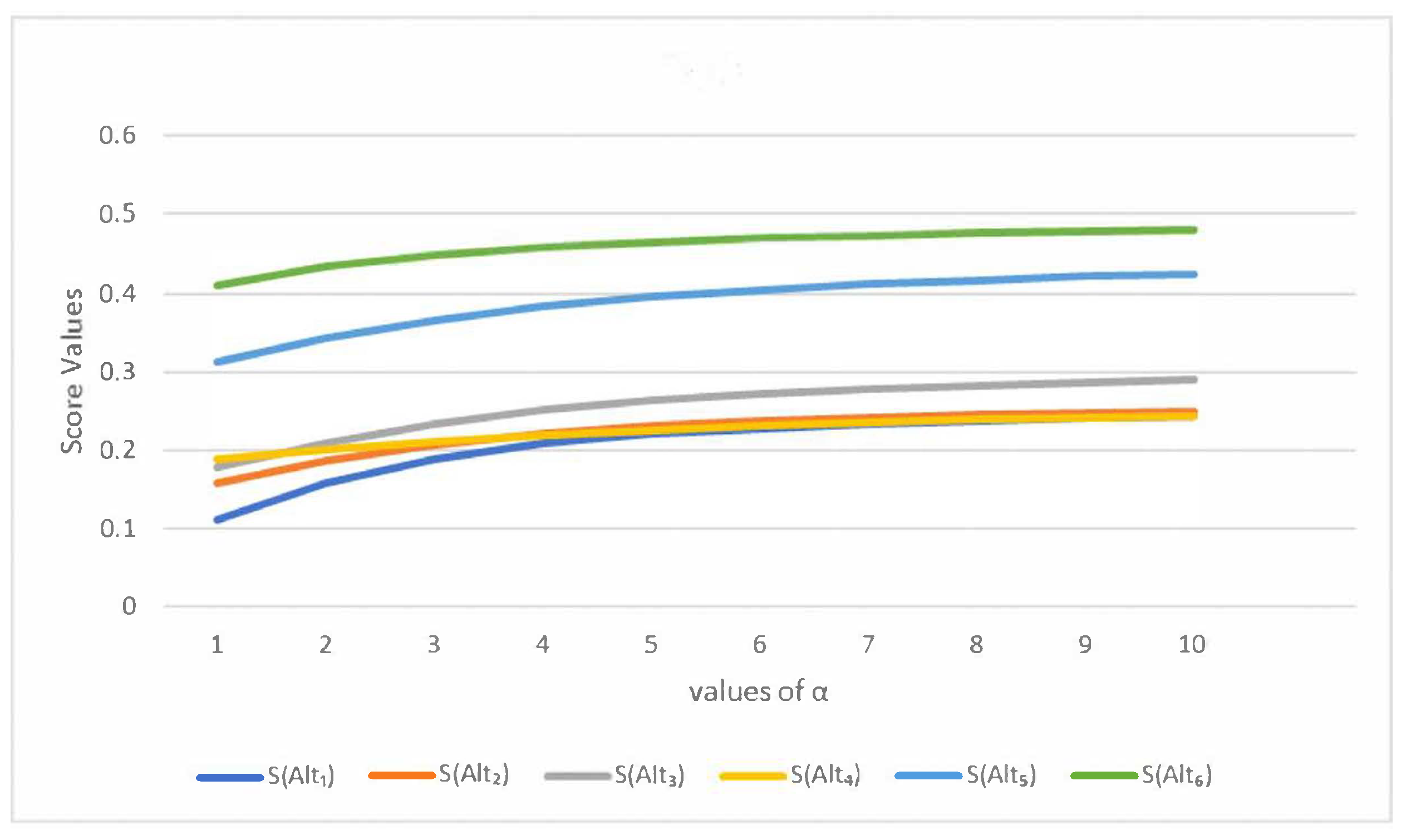
5. Analysis of the Effect of the Parameters α on Decision Making

In this subsection, we will further discuss the effect of the parameter α on the final ranking result of this example, and then we adopt the different values of the parameter α to rank the alternatives.
We examine the flexibility and advantages of the parameter α by varying its values in the SFCDWA and SFCDWG operators. In addition, we rank each alternative based on its cumulative information. We carry out the ranking outcomes for every choice for 1 α 10 . From Table 4, we can see that for different values of the parameter α the ranking orders are same.

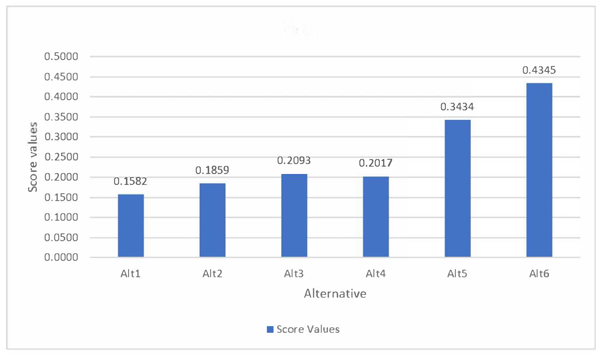
5.1. Decision Making with the SFCDWA Operator

The data in Table 4 depict the effect of parameter α on the outcome of multiple attribute decision making (MADM) when employing the SFCDWA operator. As α increases from 1 to 10, the scores of the alternatives ( A l t 1 to A l t 6 ) exhibit a pattern of change. Notably, alternative A l t 6 consistently maintains the highest score across all α values, suggesting its superiority in the decision-making process. Additionally, Table 4 visually depicts the ranking results obtained by the SFCDWA operator of α in the range [ 1 10 ] .
Figure 3 shows graphically the ranking of alternatives from Table 4.
The best alternative is A l t 6 . The obtained results utilizing spherical fuzzy credibility Dombi aggregation operators give close study about the ranking of different values of parameters. Hence, novel spherical fuzzy credibility Dombi aggregation operators are more effective and reliable to solve the group decision-making problems (Figure 3).

5.2. Decision Making with the SFCFWG Operator

The data in Table 5 depict the effects of parameter α on the outcome of multiple attribute decision making (MADM) when employing the SFCDWG operator. Across the range of α values from 1 to 10, the scores of the alternatives ( A l t 1 to A l t 6 ) exhibit a pattern of change. Notably, alternative A l t 6 consistently maintains the highest score across all α values, suggesting its superiority in the decision-making process. Additionally, Table 5 visually depicts the ranking results obtained by the SFCDWG operator of α in the range [ 1 10 ] .
Figure 4 shows graphically the ranking of alternatives from Table 5.
The best alternative is A l t 6 . The obtained results utilizing spherical fuzzy credibility Dombi aggregation operators give close study about the ranking of different values of parameters. Hence, novel spherical fuzzy credibility Dombi aggregation operators are more effective and reliable to solve the group decision-making problems (Figure 4).

6. Comparison

For the evaluation comparisons, we must compare our suggested approach with the other approaches that are currently in use in this part of the paper to confirm the correctness of our work. Consequently, two methods of comparison are available: technique-wise and aggregation operator-wise. Aggregation operators using various forms of spherical fuzzy data are being studied. We now have to compare our results with spherical fuzzy data. In the present technique, the data are spherical fuzzy numbers, and the operational rules of these numbers are used to construct a set of aggregation operators. There are various aggregation operators of that kind [33,47,48] in that sequence. Our results cannot be compared with the aforementioned finding when the data were collected as spherical fuzzy credibility numbers. We, thus, ignore the credibility terms of the MD, NuMD, and NMD.
There is a significant difference between the ranking results of the proposed method and those of the existing methods. The comparison of the proposed methods and existing techniques are discussed as follows:
  • It is clear from Table 6 that the established spherical fuzzy credibility MADM technique based on the SFCDWA and SFCDWA operators and the standard spherical fuzzy MADM [33] approach based on the SFNWAA and SFNWAG operators have different ranking outcomes. According to the decision-making example’s final outcomes, A l t 6 , which corresponds to the proven spherical fuzzy credibility MADM strategy, and A l t 5 , which corresponds to the traditional spherical fuzzy MADM approach without the degrees of credibility, are the best options.
  • It is evident from Table 6 that there is a difference in the ranking results between the established MADM method based on the SFCDWA and SFCDWA operators and the conventional spherical fuzzy MADM [47] approach based on the SFDWAA and SFDWAG operators. As per the decision-making example’s final results, A l t 6 , which aligns with the established spherical fuzzy credibility MADM approach, is the best alternative. On the other hand, A l t 3 , which is based on the SFDWAG operator, and A l t 5 , which is based on the SFDWAA operator, are the best alternatives, and they correspond to the traditional fuzzy MADM approach that lacks credibility.
  • Table 6 make it clear that the established MADM method based on the SFCDWA and SFCDWA operators and the conventional spherical fuzzy MADM [48] approach based on the SFDPWAA and SFDPWAG operators have different ranking outcomes. According to the decision-making example’s final results, A l t 6 , which corresponds to the well-established SFC MADM approach, is the best option. Alternatively, A l t 3 , based on the SFDPWAA operator, and A l t 5 , based on the SFDPWAG operator, correspond to the traditional fuzzy MADM approach without the degrees of credibility.
In order to represent the applicability and efficacy of the proven MADM technique in the context of FCNs, the degrees of credibility in the MADM problem might thus have an impact on the ranking results of the alternatives and the best choice. Consequently, the established MADM technique is better than the traditional fuzzy MADM approach.

7. Conclusions

This study introduces an innovative prolongation of the spherical fuzzy number called the spherical fuzzy credibility number (SFCN). The SFCN is defined by a trio of values (MD, NuMD, NMD) with their degree of credibility, within the context of real-world ambiguity and uncertainty. The study proceeds to present a function to find the score of SFCN and introduces the SFCDWA and SFCDWG operators as associated with SFCNs.
Subsequently, a multiple attribute decision-making (MADM) approach employing the SFCDWA and SFCDWG operators is developed to address MADM problems within the framework of SFCNs. The suggested data are operationalized in a practical decision-making example involving artificial intelligence symmetry. The goal is to illustrate the effectiveness and efficacy of the suggested data of SFCNs.
Employing a comparative examination, the study demonstrates that incorporating credibility measures into the decision-making process can influence alternative ranking, emphasizing their significance and essential role in MADM problems. The key benefit of this study lies in the proposition that the suggested information of SFCNs not only enriches the information gathered during the assessment but also improves decision efficiency in MADM problems.
From the complexity of our introduced notions, our study is also limited because if the decision makers use 0.6 as MD, 0.6 as NuMD, and 0.6 as NMD, then our proposed approach cannot handle that kind of information because the sum ( 0.36 , 0.36 , 0.36 ) [ 0 , 1 ] . Therefore, our developed approach is limited.
Future research on T-spherical credibility fuzzy sets, complex spherical credibility fuzzy sets, and complex T-spherical credibility fuzzy sets is anticipated. In order to tackle the challenges in decision making, the recommended aggregation operator may also be adjusted utilizing the Yager and Archimedean norms.

Author Contributions

Conceptualization, M.Q., N.K. and M.R.; Methodology, M.Q., D.K., M.A. and I.D.; Validation, D.K.; Formal analysis, D.S.; Investigation, M.Q.; Writing—original draft, M.Q. and M.R.; Writing—review and editing, N.K. and D.S.; Supervision, D.K. All authors contributed equally. All authors have read and agreed to the published version of the manuscript.

Funding

This research has not received any external funding.

Data Availability Statement

All the data are included in the paper.

Acknowledgments

College of Global Business, Korea University, Sejong 30019, Republic of Korea.

Conflicts of Interest

The authors declare no conflicts of interest.

References

  1. Chertok, M.; Keller, Y. Spectral symmetry analysis. IEEE Trans. Pattern Anal. Mach. Intell. 2010, 32, 1227–1238. [Google Scholar] [CrossRef]
  2. Parui, S.K.; Majumder, D.D. Symmetry analysis by computer. Pattern Recognit. 1983, 16, 63–67. [Google Scholar] [CrossRef]
  3. Belokoneva, E.L. Borate crystal chemistry in terms of the extended OD theory: Topology and symmetry analysis. Crystallogr. Rev. 2005, 11, 151–198. [Google Scholar] [CrossRef]
  4. Zadeh, L.A. Fuzzy logic-a personal perspective. Fuzzy Sets Syst. 2015, 281, 4–20. [Google Scholar] [CrossRef]
  5. Zhang, S.; Hou, Y.; Zhang, S.; Zhang, M. Fuzzy control model and simulation for nonlinear supply chain system with lead times. Complexity 2017, 2017, 2017634. [Google Scholar] [CrossRef]
  6. Zhang, S.; Zhang, C.; Zhang, S.; Zhang, M. Discrete switched model and fuzzy robust control of dynamic supply chain network. Complexity 2018, 2018, 3495096. [Google Scholar] [CrossRef]
  7. Sarwar, M.; Li, T. Fuzzy fixed point results and applications to ordinary fuzzy differential equations in complex valued metric spaces. Hacet. J. Math. Stat. 2019, 48, 1712–1728. [Google Scholar] [CrossRef]
  8. Gao, M.; Zhang, L.; Qi, W.; Cao, J.; Cheng, J.; Kao, Y.; Wei, Y.; Yan, X. SMC for semi-Markov jump TS fuzzy systems with time delay. Appl. Math. Comput. 2020, 374, 125001. [Google Scholar]
  9. Xia, Y.; Wang, J.; Meng, B.; Chen, X. Further results on fuzzy sampled-data stabilization of chaotic nonlinear systems. Appl. Math. Comput. 2020, 379, 125225. [Google Scholar] [CrossRef]
  10. Lu, K.P.; Chang, S.T.; Yang, M.S. Change-point detection for shifts in control charts using fuzzy shift change-point algorithms. Comput. Ind. Eng. 2016, 93, 12–27. [Google Scholar] [CrossRef]
  11. Ruspini, E.H.; Bezdek, J.C.; Keller, J.M. Fuzzy clustering: A historical perspective. IEEE Comput. Intell. 2019, 14, 45–55. [Google Scholar] [CrossRef]
  12. Yang, M.S.; Sinaga, K.P. Collaborative feature-weighted multi-view fuzzy c-means clustering. Pattern Recognit. 2021, 119, 108064. [Google Scholar] [CrossRef]
  13. Zhang, S.; Zhang, P.; Zhang, M. Fuzzy emergency model and robust emergency strategy of supply chain system under random supply disruptions. Complexity 2019, 2019, 3092514. [Google Scholar] [CrossRef]
  14. Atanassov, K.T.; Atanassov, K.T. Intuitionistic Fuzzy Sets; Physica-Verlag HD: Heidelberg, Germany, 1999; pp. 1–137. [Google Scholar]
  15. Hwang, C.M.; Yang, M.S. New Construction for Similarity Measures between Intuitionistic Fuzzy Sets Based on Lower, Upper and Middle Fuzzy Sets. Int. J. Fuzzy Syst. 2013, 15, 359. [Google Scholar]
  16. Yang, M.S.; Hussain, Z.; Ali, M. Belief and plausibility measures on intuitionistic fuzzy sets with construction of belief-plausibility TOPSIS. Complexity 2020, 2020, 7849686. [Google Scholar] [CrossRef]
  17. Alkan, N.; Kahraman, C. Continuous intuitionistic fuzzy sets (CINFUS) and their AHP&TOPSIS extension: Research proposals evaluation for grant funding. Appl. Soft Comput. 2023, 145, 110579. [Google Scholar]
  18. Atanassov, K.T. Circular intuitionistic fuzzy sets. J. Intell. Fuzzy Syst. 2020, 39, 5981–5986. [Google Scholar] [CrossRef]
  19. Xu, C.; Wen, Y. New measure of circular intuitionistic fuzzy sets and its application in decision making. AIMS Math. 2023, 8, 24053–24074. [Google Scholar] [CrossRef]
  20. Alreshidi, N.A.; Shah, Z.; Khan, M.J. Similarity and entropy measures for circular intuitionistic fuzzy sets. Eng. Artif. Intell. 2024, 131, 107786. [Google Scholar] [CrossRef]
  21. Yager, R.R.; Abbasov, A.M. Pythagorean membership grades, complex numbers, and decision making. Int. J. Intell. Syst. 2013, 28, 436–452. [Google Scholar] [CrossRef]
  22. Meng, Z.; Lin, R.; Wu, B. Multi-criteria group decision making based on graph neural networks in Pythagorean fuzzy environment. Expert Syst. Appl. 2024, 242, 122803. [Google Scholar] [CrossRef]
  23. Akram, M.; Nawaz, H.S.; Deveci, M. Attribute reduction and information granulation in Pythagorean fuzzy formal contexts. Expert Syst. Appl. 2023, 222, 119794. [Google Scholar] [CrossRef]
  24. Salari, S.; Sadeghi-Yarandi, M.; Golbabaei, F. An integrated approach to occupational health risk assessment of manufacturing nanomaterials using Pythagorean Fuzzy AHP and Fuzzy Inference System. Sci. Rep. 2024, 14, 180. [Google Scholar] [CrossRef] [PubMed]
  25. Yager, R.R. Generalized orthopair fuzzy sets. IEEE Trans. Fuzzy Syst. 2016, 25, 1222–1230. [Google Scholar] [CrossRef]
  26. Liu, P.; Wang, P. Some q-rung orthopair fuzzy aggregation operators and their applications to multiple-attribute decision making. Int. J. Intell. Syst. 2018, 33, 259–280. [Google Scholar] [CrossRef]
  27. Yang, M.S.; Ali, Z.; Mahmood, T. Three-way decisions based on q-rung orthopair fuzzy 2-tuple linguistic sets with generalized Maclaurin symmetric mean operators. Mathematics 2021, 9, 1387. [Google Scholar] [CrossRef]
  28. Alcantud, J.C.R. Complemental fuzzy sets: A semantic justification of $ q $-rung orthopair fuzzy sets. IEEE Trans. Fuzzy Syst. 2023, 31, 4262–4270. [Google Scholar] [CrossRef]
  29. Cuong, B.C.; Kreinovich, V. Picture fuzzy sets-a new concept for computational intelligence problems. In Proceedings of the 2013 IEEE Third World Congress on Information and Communication Technologies (WICT 2013), Hanoi, Vietnam, 15–18 December 2013; pp. 1–6. [Google Scholar]
  30. Jana, C.; Senapati, T.; Pal, M.; Yager, R.R. Picture fuzzy Dombi aggregation operators: Application to MADM process. Appl. Soft Comput. 2019, 74, 99–109. [Google Scholar] [CrossRef]
  31. Singh, S.; Ganie, A.H. Applications of picture fuzzy similarity measures in pattern recognition, clustering, and MADM. Expert. Appl. 2021, 168, 114264. [Google Scholar] [CrossRef]
  32. Ganie, A.H.; Singh, S. An innovative picture fuzzy distance measure and novel multi-attribute decision-making method. Complex Intell. Syst. 2021, 7, 781–805. [Google Scholar] [CrossRef]
  33. Ashraf, S.; Abdullah, S.; Mahmood, T.; Ghani, F.; Mahmood, T. Spherical fuzzy sets and their applications in multi-attribute decision making problems. J. Intell. Fuzzy Syst. 2019, 36, 2829–2844. [Google Scholar] [CrossRef]
  34. Aydoğdu, A.; Gül, S. A novel entropy proposition for spherical fuzzy sets and its application in multiple attribute decision-making. Int. J. Intell. Syst. 2020, 35, 1354–1374. [Google Scholar] [CrossRef]
  35. Sarfraz, M.; Pamucar, D. A parametric similarity measure for spherical fuzzy sets and its applications in medical equipment selection. J. Eng. Manag. Syst. Eng. 2024, 3, 38–52. [Google Scholar] [CrossRef]
  36. Onar, S.C.; Kahraman, C.; Oztaysi, B. Multi-criteria spherical fuzzy regret based evaluation of healthcare equipment stocks. J. Intell. Fuzzy Syst. 2020, 39, 5987–5997. [Google Scholar] [CrossRef]
  37. Ye, J.; Song, J.; Du, S.; Yong, R. Weighted aggregation operators of fuzzy credibility numbers and their decision-making approach for slope design schemes. Comput. Appl. Math. 2021, 2021, 1–14. [Google Scholar] [CrossRef]
  38. Qiyas, M.; Madrar, T.; Khan, S.; Abdullah, S.; Botmart, T.; Jirawattanapaint, A. Decision support system based on fuzzy credibility Dombi aggregation operators and modified TOPSIS method. AIMS Math. 2022, 7, 19057–19082. [Google Scholar] [CrossRef]
  39. Midrar, T.; Khan, S.; Abdullah, S.; Botmart, T. Entropy based extended TOPOSIS method for MCDM problem with fuzzy credibility numbers. AIMS Math. 2022, 7, 17286–17312. [Google Scholar] [CrossRef]
  40. Yahya, M.; Abdullah, S.; Qiyas, M. Analysis of medical diagnosis based on fuzzy credibility Dombi Bonferroni mean operator. J. Ambient. Intell. Humaniz. Comput. 2023, 14, 12709–12724. [Google Scholar] [CrossRef]
  41. Qiyas, M.; Khan, N.; Naeem, M.; Abdullah, S. Intuitionistic fuzzy credibility Dombi aggregation operators and their application of railway train selection in Pakistan. AIMS Math. 2023, 8, 6520–6542. [Google Scholar] [CrossRef]
  42. Dombi, J. A general class of fuzzy operators, the DeMorgan class of fuzzy operators and fuzziness measures induced by fuzzy operators. Fuzzy Sets Syst. 1982, 8, 149–163. [Google Scholar] [CrossRef]
  43. Khan, A.A.; Ashraf, S.; Abdullah, S.; Qiyas, M.; Luo, J.; Khan, S.U. Pythagorean fuzzy Dombi aggregation operators and their application in decision support system. Symmetry 2019, 11, 383. [Google Scholar] [CrossRef]
  44. Jana, C.; Muhiuddin, G.; Pal, M. Some Dombi aggregation of Q-rung orthopair fuzzy numbers in multiple-attribute decision making. Int. J. Intell. Syst. 2019, 34, 3220–3240. [Google Scholar] [CrossRef]
  45. Du, W.S. More on Dombi operations and Dombi aggregation operators for q-rung orthopair fuzzy values. J. Intell. Fuzzy Syst. 2020, 39, 3715–3735. [Google Scholar] [CrossRef]
  46. Seikh, M.R.; Mandal, U. Intuitionistic fuzzy Dombi aggregation operators and their application to multiple attribute decision-making. Granul. Comput. 2021, 6, 473–488. [Google Scholar] [CrossRef]
  47. Ashraf, S.; Abdullah, S.; Mahmood, T. Spherical fuzzy Dombi aggregation operators and their application in group decision making problems. J. Ambient. Intell. Humaniz. Comput. 2020, 11, 2731–2749. [Google Scholar] [CrossRef]
  48. Khan, Q.; Mahmood, T.; Ullah, K. Applications of improved spherical fuzzy Dombi aggregation operators in decision support system. Soft Comput. 2021, 25, 9097–9119. [Google Scholar] [CrossRef]
Figure 1. Ranking order of alternatives based on the SFCDWA operator.
Axioms 14 00108 g001
Figure 2. Ranking order of alternatives based on the SFCDWG operator.
Axioms 14 00108 g002
Figure 3. Ranking order of alternatives based on the SFCDWA operator.
Axioms 14 00108 g003
Figure 4. Ranking order of alternatives based on the SFCDWA operator.
Axioms 14 00108 g004
Table 1. Spherical fuzzy credibility data given by experts.
Attributes At 1 At 2 At 3 At 4
A l t 1 0.3 , 0.5 , 0.8 , 0.6 , 0.5 , 0.4 0.4 , 0.7 , 0.8 , 0.5 , 0.3 , 0.6 0.6 , 0.5 , 0.7 , 0.3 , 0.2 , 0.6 0.6 , 0.5 , 0.4 . , 0.7 , 0.6 , 0.6
A l t 2 0.7 , 0.4 , 0.6 , 0.6 , 0.3 , 0.6 0.5 , 0.5 , 0.8 , 0.4 , 0.3 , 0.5 0.7 , 0.5 , 0.6 , 0.7 , 0.3 , 0.9 0.5 , 0.7 , 0.6 , 0.8 , 0.6 , 0.7
A l t 3 0.7 , 0.7 , 0.7 , 0.8 , 0.1 , 0.6 0.6 , 0.6 , 0.7 , 0.5 , 0.3 , 0.8 0.5 , 0.7 , 0.5 , 0.8 , 0.7 , 0.6 0.6 , 0.8 , 0.3 , 0.8 , 0.7 , 0.4
A l t 4 0.6 , 0.6 , 0.5 , 0.8 , 0.6 , 0.4 0.5 , 0.8 , 0.7 , 0.7 , 0.5 , 0.7 0.7 , 0.6 , 0.5 , 0.8 , 0.4 , 0.7 0.7 , 0.4 , 0.4 , 0.8 , 0.5 , 0.7
A l t 5 0.4 , 0.7 , 0.3 , 0.7 , 0.5 , 0.7 0.7 , 0.6 , 0.5 , 0.8 , 0.3 , 0.8 0.6 , 0.8 , 0.5 , 0.6 , 0.3 , 0.7 0.6 , 0.6 , 0.6 , 0.5 , 0.4 , 0.8
A l t 6 0.6 , 0.8 , 0.3 , 0.4 , 0.6 , 0.7 0.6 , 0.7 , 0.7 , 0.6 , 0.35 , 0.8 0.7 , 0.6 , 0.5 , 0.8 , 0.5 , 0.7 0.6 , 0.8 , 0.6 , 0.6 , 0.5 , 0.8
Table 2. Aggregated results with respect to the SFCDWA and SFCDWG operators.
SFCDWA OperatorSFCDWG Operator
χ ˜ 1 0.5324 , 0.5979 , 0.5634 , 0.4388 , 0.3027 , 0.5020 0.3933 , 0.5278 , 0.5634 , 0.4388 , 0.4990 , 0.5705
χ ˜ 2 0.6500 , 0.5877 , 0.6279 , 0.5379 , 0.3260 , 0.6060 0.5690 , 0.4790 , 0.6279 , 0.5379 , 0.4712 , 0.8229
χ ˜ 3 0.6340 , 0.7297 , 0.4419 , 0.6494 , 0.6150 , 0.5321 0.5881 , 0.6812 , 0.4419 , 0.6494 , 0.6281 , 0.7021
χ ˜ 4 0.6514 , 0.7021 , 0.4849 , 0.7672 , 0.4866 , 0.5277 0.5956 , 0.5321 , 0.4849 , 0.6672 , 0.5319 . , 0.6693
χ ˜ 5 0.6178 , 0.7181 , 0.4028 , 0.6117 , 0.3526 , 0.7382 0.5104 , 0.6535 , 0.4028 , 0.6117 , 0.4207 , 0.7651
χ ˜ 6 0.6340 , 0.7645 , 0.4143 , 0.5134 , 0.4552 , 0.7382 0.6167 , 0.7036 , 0.4143 , . 0.5134 , 0.5284 , 0.7651
Table 3. Score results and positioning of alternatives based on scores.
Sc χ ˜ 1 Sc χ ˜ 2 Sc χ ˜ 3 Sc χ ˜ 4 Sc χ ˜ 5 Sc χ ˜ 6
S F C D W A 0.1582 0.1859 0.2093 0.2017 0.3434 0.4345
S F C D W G 0.1659 0.2562 0.3601 0.1804 0.3045 0.4349
Ranking
A l t 6 A l t 5 A l t 3 A l t 4 A l t 2 A l t 1
A l t 6 A l t 3 A l t 5 A l t 2 A l t 4 A l t 1
Table 4. Parameter α ’s effects on MADM outcome in relation to the SFCDWA operator.
α Sc χ ˜ 1 Sc χ ˜ 2 Sc χ ˜ 3 Sc χ ˜ 4 Sc χ ˜ 5 Sc χ ˜ 6
1 0.1110 0.1592 0.1789 0.1881 0.3130 0.4095
2 0.1582 0.1859 0.2093 0.2017 0.3434 0.4345
3 0.1895 0.2073 0.2343 0.2118 0.3666 0.4499
4 0.2085 0.2218 0.2514 0.2198 0.3835 0.4596
5 0.2205 0.2314 0.2632 0.2261 0.3958 0.4661
6 0.2284 0.2378 0.2718 0.2313 0.4050 0.4708
7 0.2340 0.2423 0.2783 0.2355 0.4119 0.4743
8 0.2382 0.2456 0.2833 0.2389 0.4173 0.4771
9 0.2414 0.2481 0.2873 0.2417 0.4216 0.4793
10 0.2440 0.2501 0.2906 0.2441 0.4251 0.4811
Ranking order
A l t 6 A l t 5 A l t 4 A l t 3 A l t 2 A l t 1
A l t 6 A l t 5 A l t 3 A l t 4 A l t 2 A l t 1
A l t 6 A l t 5 A l t 3 A l t 2 A l t 4 A l t 1
Table 5. Parameter α ’s effects on MADM outcome in relation to the SFCDWG operator.
α Sc χ ˜ 1 Sc χ ˜ 2 Sc χ ˜ 3 Sc χ ˜ 4 Sc χ ˜ 5 Sc χ ˜ 6
1 0.1177 0.2015 0.2849 0.1780 0.2923 0.4098
2 0.1659 0.2562 0.3601 0.1804 0.3045 0.4349
3 0.1957 0.2882 0.4018 0.1810 0.3142 0.4504
4 0.2134 0.3061 0.4246 0.1817 0.3216 0.4599
5 0.2246 0.3167 0.4374 0.1829 0.3272 0.4660
6 0.2322 0.3236 0.4450 0.1844 0.3314 0.4702
7 0.2376 0.3283 0.4497 0.1859 0.3347 0.4732
8 0.2417 0.3317 0.4528 0.1874 0.3373 0.4755
9 0.2449 0.3343 0.4549 0.1888 0.3393 0.4772
10 0.2475 0.3363 0.4564 0.1900 0.3410 0.4786
Ranking order
A l t 6 A l t 5 A l t 3 A l t 2 A l t 4 A l t 1
A l t 6 A l t 3 A l t 5 A l t 2 A l t 1 A l t 4
Table 6. Different aggregation operators and their ranking.
MethodsScore Values
Sc χ ˜ 1 Sc χ ˜ 2 Sc χ ˜ 3 Sc χ ˜ 4 Sc χ ˜ 5 Sc χ ˜ 6
Shahzaib et al. [33] 0.4929 0.5393 0.5807 0.5410 0.5897 0.5502
Shahzaib et al. [33] 0.4526 0.5138 0.5081 0.5305 0.5721 0.5411
Shahzaib et al. [47] 0.8900 0.7689 0.9199 0.8041 0.9045 0.8436
Shahzaib et al. [47] 0.2919 0.2852 0.4256 0.3981 0.4756 0.4646
Qaisar et al. [48] 0.5830 0.5679 0.6957 0.5715 0.6313 0.6025
Qaisar et al. [48] 0.3749 0.4570 0.4324 0.4886 0.5236 0.4958
Proposed SFCDWA 0.1582 0.1859 0.2093 0.2017 0.3434 0.4345
Proposed SFCDWG 0.1659 0.2562 0.3601 0.1804 0.3045 0.4349
Ranking
A l t 5 A l t 3 A l t 6 A l t 4 A l t 2 A l t 1
A l t 5 A l t 6 A l t 4 A l t 2 A l t 3 A l t 1
A l t 3 A l t 5 A l t 1 A l t 6 A l t 4 A l t 2
A l t 5 A l t 6 A l t 3 A l t 4 A l t 1 A l t 2
A l t 3 A l t 5 A l t 6 A l t 1 A l t 4 A l t 2
A l t 5 A l t 6 A l t 4 A l t 2 A l t 3 A l t 1
A l t 6 A l t 5 A l t 3 A l t 4 A l t 2 A l t 1
A l t 6 A l t 3 A l t 5 A l t 2 A l t 4 A l t 1
Disclaimer/Publisher’s Note: The statements, opinions and data contained in all publications are solely those of the individual author(s) and contributor(s) and not of MDPI and/or the editor(s). MDPI and/or the editor(s) disclaim responsibility for any injury to people or property resulting from any ideas, methods, instructions or products referred to in the content.

