1. Introduction
In this paper, we focus on the structured nonlinear optimization problem below:
Let
, and let
and
be closed convex sets. Consider three proper lower semi-continuous convex functions
f,
g, and
h; the function
f is differentiable, and its gradient is
-Lipschitz continuous, meaning that for all
, we have
This condition implies that the difference in function values of f at any two points in X is bounded by a constant times the Euclidean distance between those points.
It is crucial to understand that this original primal optimization problem embodies a primal-dual representation as follows:
where
denotes the conjugate of a convex function
h, defined as
The formulation in (
1) encompasses a broad spectrum of applications, such as image restoration, machine and statistical learning, compressive sensing, and portfolio optimization. Several illustrative examples are provided below:
Elastic net [
1]: The elastic net method incorporates both
and
regularization terms, leveraging the advantages of each. The elastic net estimator is defined as the solution to the following optimization problem:
where
,
,
, and
ℓ is a loss function. The second term possesses a gradient that is Lipschitz continuous. When
, the elastic net reduces to LASSO regression. Conversely, when
, the elastic net simplifies to ridge regression.
Matrix completion [
2]: Consider a matrix
with entries confined to the interval
, where
are positive real constants. The task is to recover a low-rank matrix,
X, from the observed elements of
Y. Let
be the set of
non-zero elements, and let
be a linear operator that extracts the available entries of
Y, leaving the missing entries as zeros. The problem, as defined in [
2], is formulated as the following optimization problem:
where
is a regularization constant, and
denotes the nuclear norm. By applying the Lagrange multiplier method, the aforementioned optimization task can be restated in the form presented in (
2).
Support vector machine classification [
3]: The constrained quadratic optimization problem in
can likewise be reformulated as presented in (
2).
In the dual representation of the soft-margin kernelized support vector machine classifier, we encounter a situation involving a symmetric positive semi-definite matrix , a vector , and two sets of constraints, and , within . In particular, represents a bounding constraint, and refers to a linear constraint.
Before introducing algorithms to solve (
2), we begin by reviewing several established techniques for general saddle-point problems, particularly the case of (
2), where
f is not present. Three key splitting methods are typically used:
The forward-backward-forward splitting method [
4];
The forward-backward splitting method [
5];
The Douglas-Rachford splitting method [
6].
In recent years, several primal-dual splitting algorithms have emerged, grounded in three primary foundational techniques. The primal-dual hybrid gradient (PDHG) method, first introduced in [
7], demonstrates significant numerical efficiency when applied to total variation (TV) minimization tasks. However, its convergence is highly sensitive to the choice of parameters. To mitigate this issue, Chambolle and Pock introduced the CP method in [
8], which enhances the PDHG approach by adjusting the update rule for the dual variables. This adjustment improves both convergence rates and numerical efficiency. In [
9], He and Yuan performed an extensive investigation of the CP approach, offering a comprehensive analysis via the Proximal Point Algorithm (PPA) and introducing a relaxation parameter within the PPA framework to expedite convergence (the HeYuan method). More recently, Goldstein et al. introduced the Adaptive Primal-Dual Splitting (APD) method in [
10], which dynamically modifies the step-size parameters of the CP approach. In [
11], O’Connor and Vandenberghe presented a primal-dual decomposition strategy based on Douglas-Rachford splitting, which is utilized for various primal-dual optimality condition decompositions. Additionally, the adaptive parallel primal-dual (APPD) method presented in [
12] is an enhanced version of the primal-dual approach, designed with parallel computing capabilities to optimize performance.
A comprehensive framework outlining various well-known primal-dual methods tackles the saddle-point problem by following these steps:
As summarized in
Table 1, different values of
correspond to distinct methods under the framework described in
Section 4. It is noteworthy that a straightforward correction step is necessary for both the HeYuan method and the APPD method.
In the context of (
2), Condat and Vu proposed a primal-dual splitting framework, the CV scheme, in their studies [
13,
14]. This approach, based on forward-backward iteration, extends the Chambolle-Pock algorithm (CP) by linearizing the function
f, though it operates with a narrower parameter range than CP. Later, the Asymmetric Forward-Backward-Adjoint (AFBA) splitting method, introduced in [
15], generalizes the CV scheme. Additionally, the Primal-Dual Fixed-Point (PDFP) algorithm, proposed in [
16], incorporates two proximal operations of
g in each iteration. Other notable methods for solving (
2) include the Primal-Dual Three-Operator splitting method (PD3O) from [
17] and DavisYin’s three-operator splitting technique, known as PDDY, introduced in [
18]. More recently, a modified primal-dual algorithm (MPD3O) was studied in [
19], which combines the idea of the balanced augmented Lagrangian method (BALM) in [
20] and PD3O. The parameter conditions are relaxed in [
21] for the AFBA/PDDY method.
A similar overarching framework exists for algorithms addressing (
2), analogous to the one in (
4):
The corresponding parameter restrictions for these methods are provided in
Table 2. The relationship between the aforementioned methods and the framework described in (
5) is detailed in
Table 3.
In the Discussion section of Chambolle’s work [
8], a prominent challenge for existing primal-dual methods is emphasized: the handling of a linear operator,
A, with a potentially large or unknown norm. Numerous methods, including the PDHG method described in [
7], the CP algorithm presented in [
8], the HeYuan method from [
9], the CV scheme introduced in [
13,
14], the PDFP method proposed in [
16], and the PD3O method outlined in [
17], all necessitate the satisfaction of the condition
for convergence. Consequently, the norm of
A must be computed prior to initializing the parameters. However, as the dimensionality of
A escalates, computing this norm becomes increasingly costly, thereby introducing a substantial computational burden.
To tackle the aforementioned challenge, we introduce the PPD3 algorithm, aimed at minimizing the sum of three functions, one of which includes a Lipschitz continuous term. The method we propose consists of two separate phases. In the first phase, a parallel version of (
5), where
is replaced by
, functions as a prediction step to produce an intermediate estimate. Subsequently, in the subsequent phase, the step length
is determined, after which a simple adjustment is applied to the predictor, ensuring the convergence of the PPD3 algorithm.
The key contributions presented in this paper are outlined as follows:
In contrast to other primal-dual methods, which usually update the primal and dual variables alternately, the proposed approach computes both variables simultaneously and in parallel. This parallelization can greatly accelerate computation, particularly when run on parallel computing platforms.
The proposed algorithm is independent of any prior knowledge about the linear operator A. The constraint on the parameters is no longer required. In fact, as the problem size grows, calculating the spectral norm of A, which is essential for many primal-dual methods, becomes progressively more expensive.
The step size is adjusted dynamically at each iteration. This method tailors the step size for each specific iteration, in contrast to most primal-dual approaches that employ a fixed step size constrained by a global upper limit throughout all iterations. As a result, the adaptive step size, which is typically greater, may result in faster convergence.
The organization of this paper is structured as follows: In
Section 2, we introduce the proposed algorithm.
Section 3 presents a comprehensive convergence analysis of the algorithm, while
Section 4 delves into an examination of its computational complexity.
Section 5 reports the performance of the algorithm through diverse applications, accompanied by corresponding numerical results. Lastly,
Section 6 summarizes the key conclusions and outlines potential directions for future research endeavors.
2. The Parallel Primal-Dual Algorithm
To facilitate understanding, we combine the primal and dual parameters and introduce them as follows:
The subsequent symbols are employed as well:
and
where
and
represent positive parameters. It is clear that
The concurrent primal-dual approach is described in Algorithm 1.
The loop in Algorithm 1 follows a pattern similar to the CV approach, with one key difference: the prediction step (
6) utilizes
rather than
, as seen in (
5). The incorporation of
provides a notable benefit: it eliminates the requirement for any updated data related to
x in the
y-subproblem, thus enabling the parallel processing of both the
x- and
y-subproblems.
Subsequently, the residuals
and
are calculated as termination conditions. Once both residuals tend toward zero, we will show (in the subsequent section) that
also approaches zero. Consequently, (1) converges to
By contrasting this variational inequality with (3), it is evident that
meets the criteria of the initial problem (
2). Consequently, the convergence of the primal-dual algorithm can be assessed by analyzing the residuals’ norms (see also [
10,
22,
23]).
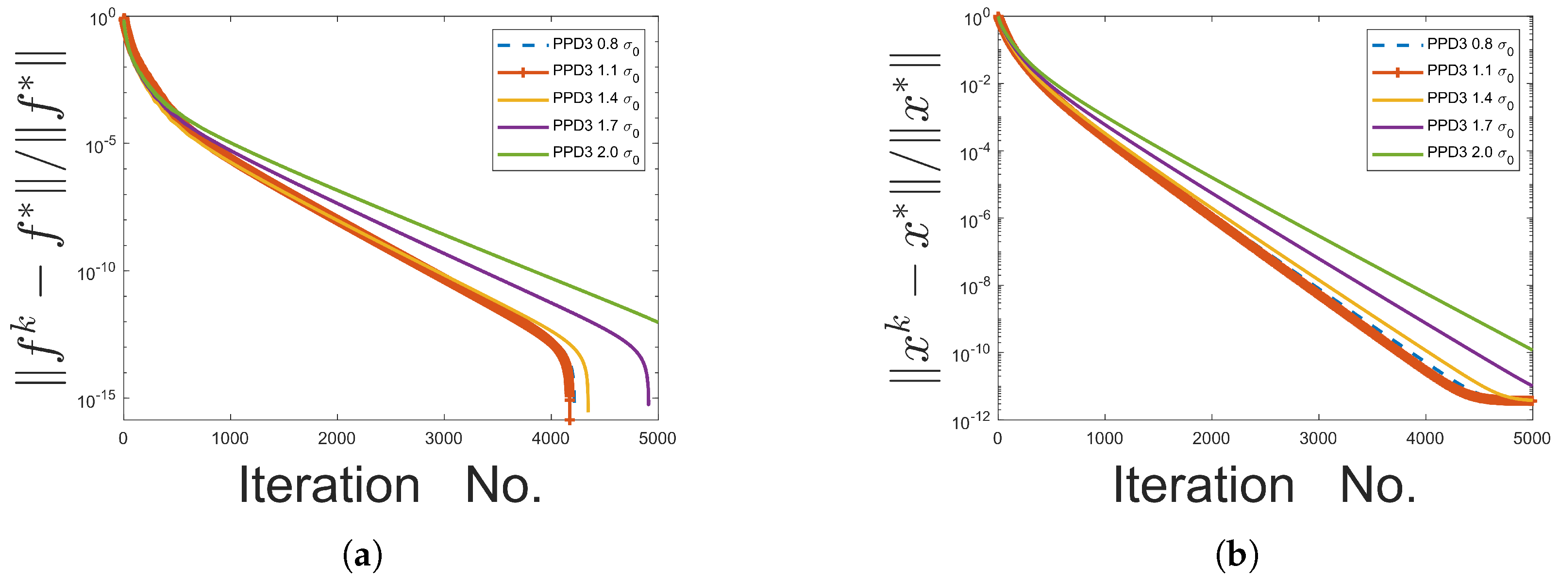
At each iteration, the step size is computed, which addresses the challenge of setting a global upper bound for the step size across all iterations. In traditional primal-dual algorithms, this upper bound is usually constrained by the condition . In contrast, our approach bypasses this limitation on the parameters and by adaptively computing . Experimental observations indicate that, in certain cases, the step size in our method exceeds the upper bound , which has been found to accelerate the convergence process.
Ultimately, a straightforward adjustment procedure guarantees the algorithm’s convergence.
| Algorithm 1: Parallel Primal-Dual Algorithm |
Initialize , , , While , > tolerance do End while
|
The prediction stage in (
6) is a special case of (
5), where
. Unlike other algorithms, such as the CV method, where
, our method uses the previous iterate
as
. When
, the prediction stage in (
6) coincides with (
4) when
.
Note that our algorithm does not require the condition for theoretical analysis, and thus, no such constraint is necessary.
6. Discussion
This paper introduces the Parallel Primal-Dual (PPD3) algorithm, a novel framework for solving optimization problems involving the minimization of the sum of three convex functions, including a Lipschitz continuous term. By leveraging parallel updates of primal and dual variables and removing stringent parameter dependencies, PPD3 addresses the computational inefficiencies inherent in existing methods. The algorithm’s adaptability to various problem settings and its ability to perform without reliance on the spectral norm of the linear operator mark notable progressions in the field of convex optimization.
In our algorithm, parallelization has the potential to accelerate computation, particularly when running on parallel computing platforms. The constraint on the parameters is removed, eliminating the need to compute the spectral norm of A, which is essential for most primal-dual methods. This also broadens the choice of parameters. Additionally, the step size is adjusted dynamically at each iteration rather than using a fixed global upper limit. As a result, our step size is typically larger, leading to faster convergence.
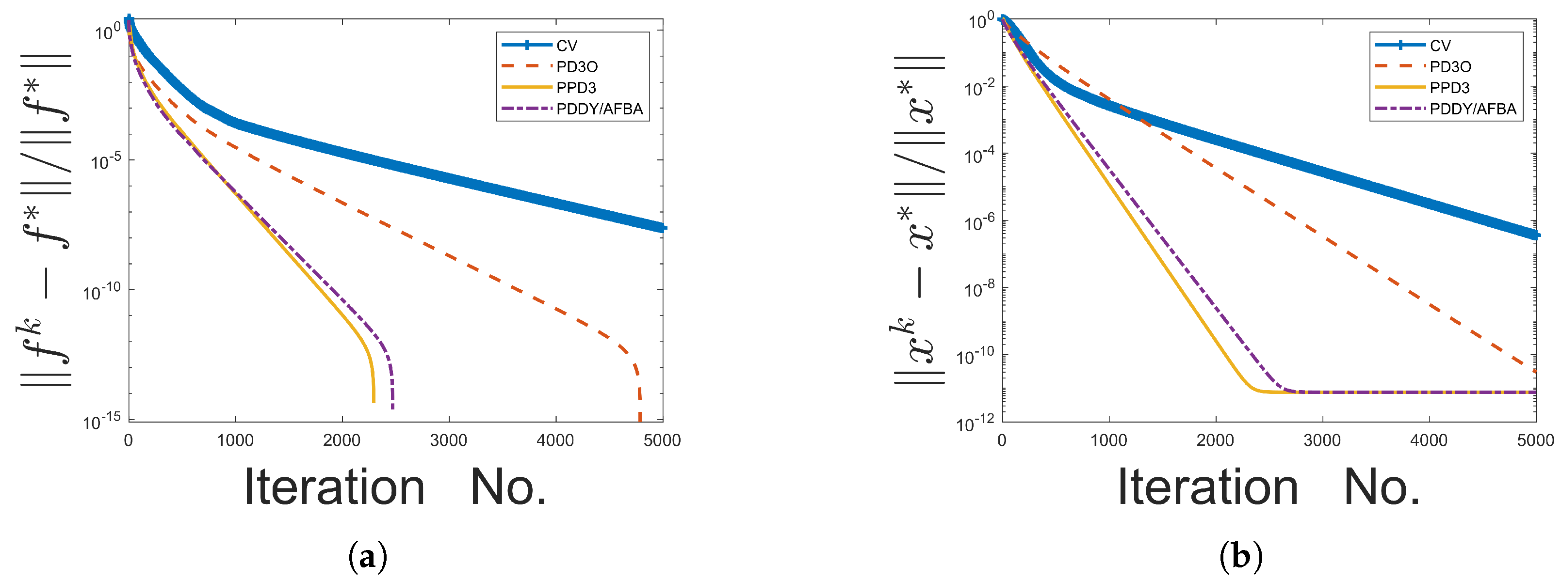
Through applications in image inpainting and Fused LASSO, PPD3 has demonstrated satisfactory performance in terms of computational efficiency and convergence speed. These results underscore its potential to handle complex, large-scale optimization challenges across a variety of domains.
For future work, we could explore extending the PPD3 framework to non-convex settings. Additionally, we may develop a stochastic version of PPD3. Furthermore, the parameters could be further investigated to determine whether they can be relaxed.


