The Law of the Iterated Logarithm for the Error Distribution Estimator in First-Order Autoregressive Models

Abstract

This paper investigates the asymptotic behavior of kernel-based estimators for the error distribution in a first-order autoregressive model with dependent errors. The model assumes that the error terms form an $\alpha$-mixing sequence with an unknown cumulative distribution function (CDF) and finite second moment. Due to the unobservability of true errors, we construct kernel-smoothed estimators based on residuals obtained via least squares. Under mild assumptions on the kernel function, bandwidth selection, and mixing coefficients, we establish a logarithmic law of the iterated logarithm (LIL) for the supremum norm difference between the residual-based kernel estimator and the true distribution function. The limiting bound is shown to be $1/2$, matching the classical LIL for independent samples. To support the theoretical results, simulation studies are conducted to compare the empirical and kernel distribution estimators under various sample sizes and error term distributions. The kernel estimators demonstrate smoother convergence behavior and improved finite-sample performance. These results contribute to the theoretical foundation for nonparametric inference in autoregressive models with dependent errors and highlight the advantages of kernel smoothing in distribution function estimation under dependence.

1. Introduction

Suppose that the sequence $\left\{X_i\right\}$ satisfies the first-order autoregressive process

$$X_i=\rho X_{i-1}+{ϵ}_i,$$

(1)

where ${ϵ}_i,i=0,\pm 1,\pm 2,\dots$, are random errors with mean 0, variance ${\sigma }_0^2>0$, and they form a weakly stationary sequence of $\alpha$-mixing with an unknown cumulative distribution function (CDF) F. Henceforth, we use the term stationary to mean weakly stationary. The definition of $\alpha$-mixing will be provided later. It is well-known that the parameter $\rho$ characterizes the properties of the process $X_i$. In this paper, we suppose $\left|\rho \right|<1$ and ${sup}_{i\ge 1}Var\left(X_i\right)<\infty$. Hence, $X_i$ is a so-called stationary process (see [1]). Throughout this paper, we consider the stationary solution of the first-order autoregressive process, which can be represented as

$$X_i=\sum _{j=0}^{\infty }{\rho }^j{ϵ}_{i-j}.$$

(2)

If ${ϵ}_1,{ϵ}_2,\dots ,{ϵ}_n,$ were observed, then the estimation of their CDF, F, can be obtained by the empirical CDF as follows:

$$F_n\left(t\right)={\displaystyle \frac{1}{n}}\sum _{i=1}^{n}I({ϵ}_i\le t),t\in \mathbb{R}.$$

(3)

For any t, $F_n\left(t\right)$ is the uniformly minimum variance unbiased estimator of $F\left(t\right)$ for all continuous distribution functions, F. It is also well known as the Glivenko–Cantelli theorem that

$$\underset{t\in \mathbb{R}}{sup}|F_n\left(t\right)-F\left(t\right)|\to 0,\mathrm{a}.\mathrm{s}.,$$

where “a.s.” stands for “almost surely” (see Gut [2]). The law of the iterated logarithm (LIL) for $F_n\left(t\right)$, i.e.,

$$\underset{n\to \infty }{lim\; sup}\sqrt{{\displaystyle \frac{n}{2log(logn)}}}\underset{t\in \mathbb{R}}{sup}|F_n\left(t\right)-F\left(t\right)|={\displaystyle \frac{1}{2}},\mathrm{a}.\mathrm{s}.$$

was obtained by Smirnov [3] and, independently, Chung [4]. Cai and Roussas [5] extended LIL of $F_n\left(t\right)$ to the case that ${ϵ}_1,{ϵ}_2,\dots ,{ϵ}_n$ were $\alpha$-mixing. Since the empirical distribution function is a step function and thus discontinuous, smooth estimators are often preferred to provide continuous and differentiable approximations that are more suitable for statistical inference and further analysis. Therefore, Yamato [6] proposed the following kernel estimator:

$$F_{nh}\left(t\right)={\displaystyle \frac{1}{n}}\sum _{i=1}^n{\int }_{-\infty }^t{K}_h(u-{ϵ}_i)du,t\in \mathbb{R},$$

(4)

where $K_h\left(u\right)=K(u/h)/h$, h is the bandwidth and K is a kernel probability density function (PDF). Cai and Roussas [5] also studied the uniform strong rate of convergence for ${sup}_{t\in \mathbb{R}}|F_{nh}\left(t\right)-F\left(t\right)|=O\left({(log(logn)/n)}^{1/2}\right)$; a.s., Cheng [7] obtained the uniform strong rate of convergence for ${sup}_{t\in \mathbb{R}}{n}^{\alpha }|F_{nh}\left(t\right)-F\left(t\right)|\to 0$, a.s., for any $0\le \alpha <1/2$.

But in autoregressive model (1), only the random variables $X_1,X_2,\dots ,X_n$ are observed. Therefore, in order to obtain an estimator of $F\left(t\right)$, we modify the definition $F_{nh}\left(t\right)$ in (4) by plugging in the residuals

$${\widehat{ϵ}}_i=X_i-{\widehat{\rho }}_n{X}_{i-1},1\le i\le n,$$

(5)

where ${\widehat{\rho }}_n={\widehat{\rho }}_n(X_1,\dots ,X_n)$ is an estimator of $\rho$. For example, the least squares estimator of $\rho$ is

$${\widehat{\rho }}_n={\displaystyle \frac{{\sum }_{i=1}^n{X}_i{X}_{i-1}}{{\sum }_{i=1}^n{X}_{i-1}^2}}.$$

Therefore, the residual empirical CDF is given by

$${\tilde{F}}_n\left(t\right)={\displaystyle \frac{1}{n}}\sum _{i=1}^{n}I({\widehat{ϵ}}_i\le t),t\in \mathbb{R},$$

(6)

and the residual kernel estimation of F is

$${\widehat{F}}_{nh}\left(t\right)={\displaystyle \frac{1}{n}}\sum _{i=1}^n{\int }_{-\infty }^t{K}_h(u-{\widehat{\epsilon }}_i)du,t\in \mathbb{R}.$$

(7)

Under the i.i.d. errors, Cheng [8] considered the first-order autoregressive model (1) and verified that the Glivenko–Cantelli theorem still holds for the estimators ${\widehat{F}}_n\left(t\right)$ and ${\widehat{F}}_{nh}\left(t\right)$, i.e.,

$$\underset{t\in \mathbb{R}}{sup}|{\widehat{F}}_n\left(t\right)-F\left(t\right)|\to 0,\underset{t\in \mathbb{R}}{sup}|{\widehat{F}}_{nh}\left(t\right)-F\left(t\right)|\to 0,\mathrm{a}.\mathrm{s}.$$

Beyond the classical LIL under the supremum norm, recent research has extended the LIL framework to other normed settings. In particular, Cheng [9] considered the first-order autoregressive model (1) and obtained the integrated absolute error (i.e., $L_1$-norm) of ${\widehat{F}}_{nh}$,

$$\underset{n\to \infty }{lim\; sup}\sqrt{{\displaystyle \frac{n}{2log(logn)}}}{\int }_{-\infty }^{\infty }|{\widehat{F}}_{nh}\left(t\right)-F\left(t\right)|dF\left(t\right)={\displaystyle \frac{\sqrt{3}}{6}},\mathrm{a}.\mathrm{s}.$$

(8)

Motivated by these findings, our work focuses on the LIL for the residual kernel estimator ${\widehat{F}}_{nh}\left(t\right)$ in the first-order autoregressive model (1) with $\alpha$-mixing errors, i.e.,

$$\underset{n\to \infty }{lim\; sup}\sqrt{{\displaystyle \frac{n}{2log(logn)}}}\underset{t\in \mathbb{R}}{sup}|{\widehat{F}}_{nh}\left(t\right)-F\left(t\right)|={\displaystyle \frac{1}{2}},\mathrm{a}.\mathrm{s}.$$

(9)

Let us recall the definition of an $\alpha$-mixing sequence.

Definition 1.

Denote $N=\{1,2,\dots ,n,\dots \}$. Let ${\mathcal{F}}_m^n=\sigma ({ϵ}_i,m\le i\le n,i\in N)$ be the σ-field generated by random variables $\{{ϵ}_m,{ϵ}_{m+1},\dots ,{ϵ}_n\},1\le m\le n$. For $n\ge 1$, we define

$$\alpha \left(n\right)=\underset{m\in N}{sup}\underset{A\in {\mathcal{F}}_1^m,B\in {\mathcal{F}}_{m+n}^{\infty }}{sup}|P\left(AB\right)-P\left(A\right)P\left(B\right)|.$$

If $\alpha \left(n\right)\downarrow 0$ as $n\to \infty$, $\{{ϵ}_n,n\ge 1\}$ is called a strong mixing or α-mixing sequence.

The $\alpha$-mixing condition is a type of weak dependence commonly used in time series analysis. It measures how quickly the dependence between past and future observations decays as the time gap increases. For more properties of $\alpha$-mixing sequences, one can refer to Györfi [10], Roussas [11], Fan and Yao [12], Wang et al. [13], etc.

For more research on LIL, one can refer to Gajek et al. [14] and Cheng [15] for $L_p$-norms of the empirical distribution function $F_n\left(t\right)$ and kernel distribution function $F_{nh}\left(t\right)$; Li and Wang [16] and Petrov [17] investigated the LIL for the sequences of dependent random variables; Liu and Zhang [18] studied the LIL for error density estimators in nonlinear autoregressive models, etc.

In the context of estimating the error distribution function, this paper makes three main contributions. First, we consider a linear first-order autoregressive model in which the autoregressive coefficient $\rho$ must be estimated rather than assumed known. Second, we study kernel-based nonparametric estimators for the error distribution, providing smoother approximations than the empirical distribution function and enabling refined probabilistic analysis. Third, we explicitly allow for dependent errors modeled by a stationary $\alpha$-mixing sequence, extending classical results beyond the independent error setting.

It is worth noting that for the i.i.d. case, the LIL for the empirical distribution function case has been well established by Smirnov [3] and Chung [4]. For kernel estimators of the error distribution, related results were obtained by Niu [19] and Cheng [20]. Our work extends these classical results to the dependent error setting, motivated in part by earlier studies on autoregressive processes such as that by Wang et al. [21], bridging the gap between the i.i.d. theory and time series models with weakly dependent innovations.

We also remark that alternative weak dependence structures could be considered. For example, if the errors are independent, the convergence rates simplify, and some technical conditions can be relaxed. If $\alpha$-mixing is replaced by other forms of weak dependence, such as $\beta$-mixing, $\rho$-mixing, or martingale difference sequences or the weak dependence framework of Doukhan and Louhichi [22], we expect similar LIL results to hold under appropriate moment and dependence assumptions, though the technical details and proof techniques would require adaptation. A full exploration of these generalizations is beyond the scope of the present paper, but they constitute interesting directions for future research.

The rest of this paper is organized as follows: in Section 2, we list some basic assumptions for the first-order autoregressive model (1). The main results of a uniform strong rate of ${sup}_{t\in \mathbb{R}}|{\widehat{F}}_{nh}\left(t\right)-F_{nh}\left(t\right)|$ and LIL of (9) are presented in Section 3. In order to check our results, some simulations are presented in Section 4. Some technical Lemmas and proofs are presented in Section 5. Last, we provide a conclusion and discussion in Section 6. Throughout the paper, we assume that limits are taken as $n\to \infty$ unless otherwise specified. The $C,C_1,\mathrm{and}{C}_2$ denote some positive constants not depending on n, which may be different in various places.

2. Assumptions

This section presents the basic assumptions required for model (1) as well as the main theorems.

(A1)

In model (1), let the sequence $\{{ϵ}_i,-\infty <i<\infty \}$ of errors form a stationary sequence of $\alpha$-mixing with unknown CDF F with a bounded second-order derivative, i.e., there exists a positive constant C ($0<C<\infty$) such that $|F^{″}\left(t\right)|\le C$ for all $t\in \mathbb{R}$. Assume $E{ϵ}_1=0$ and $E|{ϵ}_1{|}^p<\infty$ for some $p>2$. The mixing coefficient satisfies $\alpha \left(n\right)=O\left(n^{-r}\right)$, where $r>{\displaystyle \frac{5p+2}{p-2}}$.

(A2)

The kernel function $K\left(t\right),tK\left(t\right)$, and $t^{2}K\left(t\right)$ are integrable over the real line and satisfy

$$0\le \underset{t\in \mathbb{R}}{inf}K\left(t\right)\le \underset{t\in \mathbb{R}}{sup}K\left(t\right)<\infty ,{\int }_{-\infty }^{+\infty }K\left(t\right)dt=1,{\int }_{-\infty }^{+\infty }tK\left(t\right)dt=0,{\int }_{-\infty }^{+\infty }{t}^{2}K\left(t\right)dt<\infty .$$

(A3)

The bandwidth h satisfies the following conditions:

$$h\to 0,n{h}^4/log(logn)\to 0,n{h}^2/{(logn)}^2\to \infty .$$

(A4)

In model (1) with $\left|\rho \right|<1$, let the ${\widehat{\rho }}_n$ be an estimator of $\rho$ with the following almost-surely (a.s.) property: there exists a positive constant C such that

$$|{\widehat{\rho }}_n-\rho |\le C{n}^{-1/2}{(log(logn))}^{1/2},\mathrm{a}.\mathrm{s}.$$

Remark 1.

We discuss these assumptions as follows:

(i) 

Assumption (A1) contains the smoothness of the error CDF F and the boundness of its second derivative $F^{″}$. It also requires the mixing coefficients satisfy $\alpha \left(n\right)=O\left(n^{-r}\right)$, where $r>{\displaystyle \frac{5p+2}{p-2}}$ and $p>2$ (p-th moment of error). If $p\to 2$, then $r\to \infty$. It is a strong condition of mixing coefficients, which require the errors to be asymptotically independent. If $p\to \infty$, then $r\to 5$. This requires a strong p-th moment of errors. In future research, we will try to relax the mixing coefficient condition. For more properties of α-mixing sequences, one can refer to Györfi [10], Roussas [11], Fan and Yao [12], Wang et al. [13], etc.

(ii) 

Assumption (A2) is the common condition of kernel $K(·)$ about non-negatively, symmetry, and integrability. Obviously, the probability density functions Gaussian kernel $K\left(t\right)={\left(2\pi \right)}^{-{\displaystyle \frac{1}{2}}}exp(-{\displaystyle \frac{t^2}{2}})$ and Epanechnikov kernel $K\left(t\right)={\displaystyle \frac{3}{20\sqrt{5}}}(5-t^2)I(t\le \sqrt{5})$ conform to Assumption (A2). See for example, Györfi et al. [10], Roussas [11], Fan and Yao [12], Li and Racine [23], etc.

(iii) 

Assumption (A3) is a standard condition for bandwidth selection in kernel density estimation. For example, similar conditions are used by Cheng et al. [7,9,15], particularly in the proof of Lemma 5. A commonly used bandwidth is $h=n^{-1/4}$.

(iv) 

Assumption (A4) requires that the estimator $\widehat{\rho }$ of the autoregressive parameter ρ converges almost surely at the rate $O\left(n^{-1/2}{(log(logn))}^{1/2}\right)$. This condition plays a key role in our theoretical results, as it ensures that the effect of estimating ρ is asymptotically negligible. Without such a rate, the additional error introduced by residuals could dominate the behavior of the kernel estimator and invalidate the uniform LIL established in this paper. When ${ϵ}_1,{ϵ}_2,\dots ,{ϵ}_n$ are i.i.d. errors, Koul and Zhu [24] considered a generalized M-estimator for p-th order autoregression models and obtained a strong rate of convergence for M-estimators ${\widehat{\rho }}_n$, i.e., $\left|\right|{\widehat{\rho }}_n-\rho \left|\right|\le C{n}^{-1/2}{(log(logn))}^{1/2}$, a.s., including the least-squares estimator; Cheng [9] used Assumption (A4) to study the $L_1$-norm of ${\widehat{F}}_{nh}$ in (8). When ${ϵ}_1,{ϵ}_2,\dots ,{ϵ}_n$ in the first-order autoregression model (1) are α-mixing random variables with common density function f and $\left|\rho \right|<1$, Gao et al. [25] used the condition $|{\widehat{\rho }}_n-\rho |=O_p\left(n^{-1/2}\right)$ to study the asymptotic normality of the kernel density estimator ${\widehat{f}}_n\left(t\right)={\displaystyle \frac{1}{nh}}{\sum }_{i=1}^n{K}_h(u-{\widehat{\epsilon }}_i)$ for the error density function f. Wu et al. [26] extended the work to nonlinear autoregressive models. In the proof by Gao et al. [25], moment inequalities were used to establish the convergence in probability. However, to extend these results to almost-sure convergence, it would be necessary to employ exponential inequalities. This in turn requires additional conditions on the α-mixing coefficients, ensuring that the covariance structure of the α-mixing sequence satisfies certain summability and decay properties. The proof of such a result is highly technical and involves delicate handling of the dependence structure. Because this is beyond the scope of the present paper, we treat Assumption (A4) as a standing assumption rather than providing a full proof here, and we leave this as an important topic for our future research.

3. Main Results

We now present the first main result of this section, which describes the uniform strong rate of convergence between ${\widehat{F}}_{nh}\left(t\right)$ and $F_{nh}\left(t\right)$ in the stationary autoregressive model (1).

Theorem 1.

In the model (1), let Assumptions (A1)–(A4) hold. Then

$$\sqrt{{\displaystyle \frac{n}{log(logn)}}}\underset{t\in \mathbb{R}}{sup}|{\widehat{F}}_{nh}\left(t\right)-F_{nh}\left(t\right)|=o\left(1\right),\mathrm{a}.\mathrm{s}.$$

where ${\widehat{F}}_{nh}\left(t\right)$ is defined in (7) and $F_{nh}\left(t\right)$ is defined by (6).

By Theorem 1, one can get the uniform strong rate

$$\underset{t\in \mathbb{R}}{sup}|{\widehat{F}}_{nh}\left(t\right)-F_{nh}\left(t\right)|=o\left({(log(logn)/n)}^{1/2}\right),\mathrm{a}.\mathrm{s}.$$

Combining the LIL of $F_{nh}\left(t\right)$ in Lemma 6, i.e.,

$$\underset{n\to \infty }{lim\; sup}\sqrt{{\displaystyle \frac{n}{2log(logn)}}}\underset{t\in \mathbb{R}}{sup}|F_{nh}\left(t\right)-F\left(t\right)|={\displaystyle \frac{1}{2}},\mathrm{a}.\mathrm{s}.,$$

we present the LIL for the residual kernel estimator ${\widehat{F}}_{nh}\left(t\right)$ as follows:

Theorem 2.

Under the same conditions as in Theorem 1, we have

$$\underset{n\to \infty }{lim\; sup}\sqrt{{\displaystyle \frac{n}{2log(logn)}}}\underset{t\in \mathbb{R}}{sup}|{\widehat{F}}_{nh}\left(t\right)-F\left(t\right)|={\displaystyle \frac{1}{2}},\mathrm{a}.\mathrm{s}.$$

Remark 2.

In Theorem 3.2 of Cai and Roussas’s study [5], Cai and Roussas obtained the LIL with α-mixing samples such that

$$\underset{n\to \infty }{lim\; sup}\sqrt{{\displaystyle \frac{n}{2log(logn)}}}\underset{t\in \mathbb{R}}{sup}|F_n\left(t\right)-F\left(t\right)|=1,\mathrm{a}.\mathrm{s}.$$

They had a typo error in estimation (17) that was equal to 1 a.s. In fact, they mistakenly cited [27] [Corollary 1.15.1] and claimed that

$$\underset{n\to \infty }{lim\; sup}[{\displaystyle \frac{1}{n}}\sqrt{{\displaystyle \frac{n}{2log(logn)}}}\underset{t\in \mathbb{R}}{sup}\left|K(t,n)\right|]=1,\mathrm{a}.\mathrm{s}.$$

But it is

$$\underset{n\to \infty }{lim\; sup}[{\displaystyle \frac{1}{n}}\sqrt{{\displaystyle \frac{n}{2log(logn)}}}\underset{t\in \mathbb{R}}{sup}\left|K(t,n)\right|]={\displaystyle \frac{1}{2}},\mathrm{a}.\mathrm{s}.,$$

(see the proof of Lemma 4). Thus, Theorem 2 extends the conclusion of LIL to the kernel estimator ${\widehat{F}}_{nh}\left(t\right)$ of error CDF $F\left(t\right)$ in autoregressive model (1) based on α-mixing errors.

4. Simulations

To verify the theoretical results, we conduct simulation studies to assess the uniform convergence behavior of four distribution estimators under different error distribution settings, namely Gaussian and Gamma. The goal is to compare the accuracy of these estimators in approximating the true error distribution function, particularly in terms of the iterated logarithm convergence rate.

We consider the first-order autoregressive model:

$$X_i=0.5X_{i-1}+{ϵ}_i,1\le i\le n,$$

where $\left\{{ϵ}_i\right\}$ is a dependent error sequence following either a Gaussian distribution or a Gamma distribution.

• Gaussian errors: $ϵ\sim N(0,{\Sigma }_n)$, where ${\Sigma }_n$ is a Toeplitz covariance matrix with entries ${|i-j|}^{-3}$, ensuring that the errors form an $\alpha$-mixing sequence. A Toeplitz matrix is a matrix in which each descending diagonal from left to right is constant. For more details about the Toeplitz matrix, we can refer to Trench [28]. As discussed in [29], it is easy to check that ${ϵ}_1,{ϵ}_2,\dots$ are $\alpha$-mixing with $\alpha \left(n\right)=O\left(n^{-3}\right)$.
• Gamma errors: we adopt a Gaussian copula-based approach to generate random vectors with exact Gamma marginals and an approximately specified covariance matrix. Specifically, we first generate a multivariate normal vector $Z\sim N(0,R)$, where R is the correlation matrix corresponding to the target covariance matrix ${\Sigma }_n$. Each component of Z is then transformed to a uniform random variable via the standard normal CDF and is subsequently mapped to a Gamma(4,1) random variable using the Gamma inverse CDF. This method guarantees the correct marginal Gamma distribution, while the resulting sample covariance matrix is very close to ${\Sigma }_n$, with only small differences. An exact covariance match can be achieved using the NORTA (Normal To Anything) method, which iteratively adjusts the Gaussian correlation matrix to perfectly reproduce the target covariance after the nonlinear transformation. However, NORTA is computationally intensive, so we do not adopt it here, given that the Gaussian copula-based approach already provides sufficient accuracy and efficiency.

For each sample size $n\in \{300,600,2000,3000,4000,5000\}$, we perform 100 Monte Carlo simulations. In each replication, the following four estimators of the error distribution function are constructed:

• $F_n\left(t\right)$: empirical distribution function based on the true errors;
• $F_{nh}\left(t\right)$: kernel-smoothed distribution estimator based on true errors;
• ${\tilde{F}}_n\left(t\right)$: empirical distribution based on residuals (from least squares estimation);
• ${\widehat{F}}_{nh}\left(t\right)$: kernel-smoothed distribution based on residuals (from least-squares estimation).

To measure the estimation accuracy, we compute the Kolmogorov–Smirnov (KS) distance between each estimator and the true distribution function and normalize it using the theoretical upper bound under the law of the iterated logarithm:

$$NKS=\sqrt{{\displaystyle \frac{n}{2log(logn)}}}\mathrm{KS}\mathrm{distance}.$$

Define the NKS for the estimators,

$$\begin{array}{cc}\hfill NK{S}_1& =\sqrt{{\displaystyle \frac{n}{2log(logn)}}}\underset{t\in \mathbb{R}}{sup}|F_n\left(t\right)-F\left(t\right)|,\hfill \\ \hfill NK{S}_2& =\sqrt{{\displaystyle \frac{n}{2log(logn)}}}\underset{t\in \mathbb{R}}{sup}|F_{nh}\left(t\right)-F\left(t\right)|,\hfill \\ \hfill NK{S}_3& =\sqrt{{\displaystyle \frac{n}{2log(logn)}}}\underset{t\in \mathbb{R}}{sup}|{\tilde{F}}_n\left(t\right)-F\left(t\right)|,\hfill \\ \hfill NK{S}_4& =\sqrt{{\displaystyle \frac{n}{2log(logn)}}}\underset{t\in \mathbb{R}}{sup}|{\widehat{F}}_{nh}\left(t\right)-F\left(t\right)|.\hfill \end{array}$$

A Gaussian kernel is used for smoothing, with bandwidth $h=n^{-1/3}$. The estimators are evaluated over the range $t\in [-3,3]$.

To investigate the effect of the bandwidth h on the performance of the proposed kernel estimator, we conducted a sensitivity analysis for two representative sample sizes, $n=600$ and $n=3000$. For $n=600$, the bandwidth h was taken from the set $\{0.01,0.05,0.10,0.15,0.20,0.202,0.25,0.30,0.35,0.40\}$, where $h=0.202$ corresponds exactly to the suggested choice $n^{-1/4}$ with $n=600$. For $n=3000$, the bandwidth h was chosen from the set $\{0.01,0.05,0.10,0.135,0.15,0.20,0.25,0.30,0.35,0.40\}$, where $h=0.13$ corresponds to the suggested choice $n^{-1/4}$ with $n=3000$.

Figure 1 and Figure 2 present the corresponding boxplots of the statistic $NK{S}_4$ for these different bandwidths under the Gaussian error setting, with Figure 1 corresponding to the sample size $n=600$ and Figure 2 corresponding to the sample size $n=3000$. For $n=600$, although there is mild fluctuation across different bandwidths, the boxplot corresponding to $h=0.202=n^{-1/4}$ shows that its median is closer to zero and the interquartile range is under 0.5, indicating that the estimator performs more stably and with less bias at this recommended bandwidth. For $n=3000$, the variability of $NK{S}_4$ across bandwidths is smaller. Again, the boxplot for $h=0.135=n^{-1/4}$ is closer to zero, further supporting the theoretical bandwidth selection. These findings confirm that $NKS4$ is not sensitive to bandwidth variation, and they provide strong empirical evidence that the bandwidth $h=n^{-1/4}$ offers a good kernel estimator for CDF F. Therefore, all subsequent simulation results reported in this paper are based on the bandwidth $h=n^{-1/4}$ to ensure consistency and comparability across experiments. Figure 3, Figure 4, Figure 5 and Figure 6 display boxplots of $NKS$ across different sample sizes and estimation methods. Each sample size includes 100 simulation replicates per method. The vertical axis represents the NKS, and a horizontal dashed line at level 0.5 is included to indicate the asymptotic upper bound suggested by the iterated logarithm law.

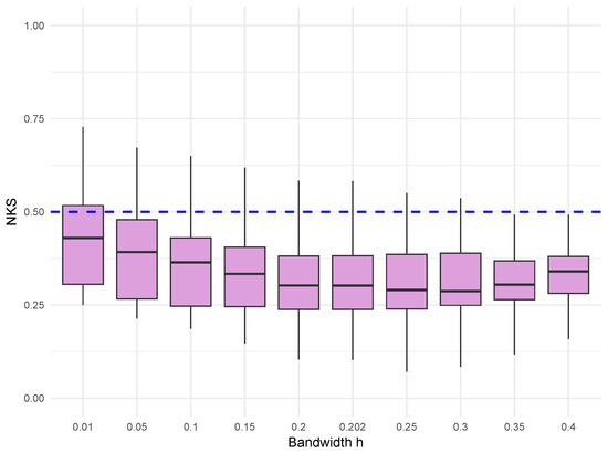
Figure 1. Boxplot of $NK{S}_4$ under different bandwidth choices for sample size $n=600$ in the Gaussian error setting.

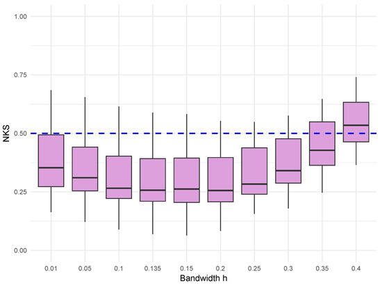
Figure 2. Boxplot of $NK{S}_4$ under different bandwidth choices for sample size $n=3000$ in the Gaussian error setting.

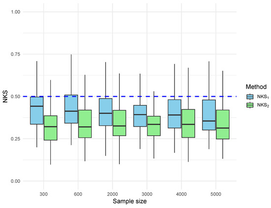
Figure 3. Boxplot of NKS distance for error-based estimators under Gaussian errors. $NK{S}_1$ and $NK{S}_2$ are the NKS distances for $F_n\left(t\right)$ and $F_{nh}\left(t\right)$, respectively.

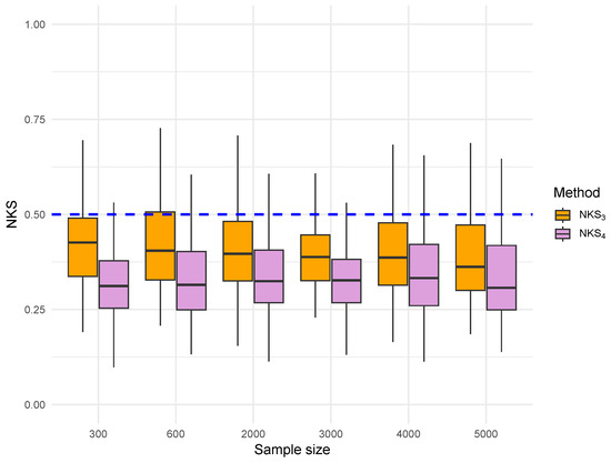
Figure 4. Boxplot of NKS distance for residual-based estimators under Gaussian errors. $NK{S}_3$ and $NK{S}_4$ are the NKS distances for ${\tilde{F}}_n\left(t\right)$ and ${\widehat{F}}_{nh}\left(t\right)$, respectively.

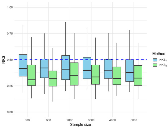
Figure 5. Boxplot of NKS distance for error-based estimators under Gamma errors. $NK{S}_1$ and $NK{S}_2$ are the NKS distances for $F_n\left(t\right)$ and $F_{nh}\left(t\right)$, respectively.

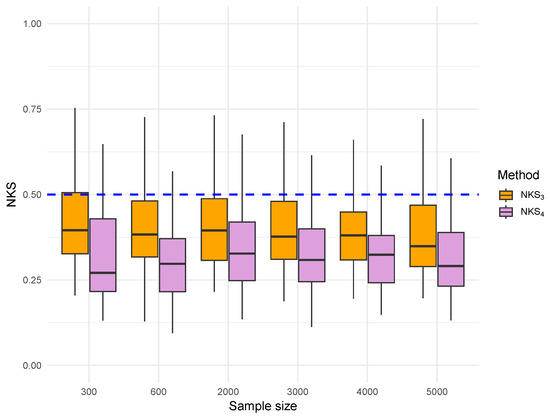
Figure 6. Boxplot of NKS distance for residual-based estimators under Gamma errors. $NK{S}_3$ and $NK{S}_4$ are the NKS distances for ${\tilde{F}}_n\left(t\right)$ and ${\widehat{F}}_{nh}\left(t\right)$, respectively.

Figure 3 presents the NKS distances for the empirical estimator $F_n\left(t\right)$ and the kernel estimator $F_{nh}\left(t\right)$, both based on true Gaussian errors. Each boxplot summarizes the distribution of NKS across 100 replications. We observe that the upper edge of the boxes (the 75th percentile) for both estimators stays well below the 0.5 theoretical boundary, even at the smallest sample size $n=300$. As the sample size increases, the entire box shrinks downward, indicating uniform improvement in estimator accuracy. The kernel estimator $F_{nh}\left(t\right)$ consistently shows a tighter spread and a lower upper quartile than $F_n\left(t\right)$, highlighting the advantage of kernel smoothing in reducing estimation variance under Gaussian error structures.

Figure 4 shows the NKS distances for the residual-based estimators ${\tilde{F}}_n\left(t\right)$ and ${\widehat{F}}_{nh}\left(t\right)$, derived from least-squares residuals under the same Gaussian error process. The results are similar to those in Figure 3. The upper quartile of the NKS remains consistently below 0.5 for both methods across all sample sizes. Again, the kernel estimator ${\widehat{F}}_{nh}\left(t\right)$ shows superior concentration, with its upper edge often well below the 0.5 threshold, even at $n=300$. This suggests that residual-based estimators, particularly when smoothed, maintain excellent uniform convergence properties under Gaussian dependence, nearly matching the performance of error-based methods.

Figure 5 and Figure 6 report the results under Gamma-distributed and dependent errors. Although the Gamma distribution is skewed and heavy-tailed, the overall performance of the estimators remains similar to that observed under Gaussian errors. All estimators exhibit convergence as the sample size increases, and kernel-based methods continue to outperform empirical ones in terms of reduced dispersion and tighter concentration around the theoretical upper bound.

The simulation results confirm the validity of the iterated logarithm law for both error-based and residual-based estimators under dependent data. Among all the methods, the kernel-based estimators consistently demonstrate superior stability and accuracy across different error distributions and sample sizes.

5. Proofs of the Main Results

Lemma 1

(Hall and Heyde [30], Corollary A.2). Suppose that ξ and η are random variables which are ${\mathcal{F}}_1^t$ and ${\mathcal{F}}_{t+\tau }^{\infty }$-measurable, respectively, $t,\tau \in \mathbb{N}$, and that ${E\left|\eta \right|}^p<\infty$, ${E\left|\xi \right|}^q<\infty$, where $p,q>1$ and ${\displaystyle \frac{1}{p}}+{\displaystyle \frac{1}{q}}<1$. Then,

$$|E\xi \eta -E\xi E\eta |\le {8\left(E\right|\xi |}^p{)}^{1/p}{\left(E\right|\eta |}^q{)}^{1/q}{\left(\alpha (\mathcal{G},\mathcal{H})\right)}^{1-{\displaystyle \frac{1}{p}}-{\displaystyle \frac{1}{q}}}.$$

Lemma 2

(Liebscher [31], Proposition 5.1). Let ${\left\{Z_n\right\}}_{n\ge 1}$ be a stationary α-mixing sequence with mixing coefficient $\alpha \left(n\right)$. Assume that $E{Z}_i=0$ and $|Z_i|\le S<\infty$, $\mathrm{a}.\mathrm{s}.$, $i=1,2,\dots ,n$. Then, for $n,h\in \mathbb{N}$, $0<h\le n/2$ and every $\epsilon >0$,

$$P\left(\left|\sum _{i=1}^n{Z}_i\right|>\epsilon \right)\le 4exp\left\{-{\displaystyle \frac{{\epsilon }^2}{16}}{(n{h}^{-1}{D}_h+{\displaystyle \frac{1}{3}}\epsilon Sh)}^{-1}\right\}+32{\displaystyle \frac{S}{\epsilon }}n\alpha \left(h\right),$$

where $D_h=\underset{1\le j\le 2h}{max}\mathrm{Var}\left({\sum }_{i=1}^j{Z}_i\right)$.

Lemma 3.

In the first-order autoregression (1), let Assumption (A1) hold. Then for any permutation $\{j_1,j_2,\dots ,j_n\}$ of $\{1,2,\dots ,n\}$, we have

$$\underset{1\le m<n}{max}\left|\sum _{k=1}^m{X}_{j_k}\right|=O(n^{1/2}logn),\mathrm{a}.\mathrm{s}.$$

(10)

Proof of Lemma 3.

Since $\left|\rho \right|<1$, by (2), the stationary process ${\left\{X_i\right\}}_{i=1}^n$ in the first-order autoregression (1) has a representation of $X_i={\sum }_{j=0}^{\infty }{\rho }^j{ϵ}_{i-j}$, $n\ge 1$. Let $I_i\left(m\right)=1$ if $i\in \{j_1,\dots ,j_m\}$ and $I_i\left(m\right)=0$ otherwise. Then,

$$\underset{1\le m\le n}{max}\left|\sum _{i=1}^n{X}_{j_i}\right|\le \underset{1\le m\le n}{max}\left|\sum _{i=1}^n{I}_i\left(m\right)\sum _{j=0}^n{\rho }^j{ϵ}_{i-j}\right|+\underset{1\le m\le n}{max}\left|\sum _{i=1}^n{I}_i\left(m\right)\sum _{j>n}{\rho }^j{ϵ}_{i-j}\right|.$$

By $p>2$, $E{ϵ}_1=0$, $E|{ϵ}_1{|}^p<\infty$, it has $Var\left({ϵ}_1\right)={\sigma }_{ϵ}^2<\infty$. According to the Chebyshev inequality and Cauchy inequality, we have

$$\begin{array}{cc}\hfill & \sum _{n=1}^{\infty }P\left(\underset{1\le m\le n}{max}\left|\sum _{i=1}^n{I}_i\left(m\right)\sum _{j>n}{\rho }^j{ϵ}_{i-j}\right|\ge n^{1/2}logn\right)\hfill \\ \hfill \le & \sum _{n=1}^{\infty }{\displaystyle \frac{1}{n{(logn)}^2}}\sum _{m=1}^{n}E{\left(\sum _{i=1}^n{I}_i\left(m\right)\sum _{j>n}{\rho }^j{ϵ}_{i-j}\right)}^2\hfill \\ \hfill \le & \sum _{n=1}^{\infty }{\displaystyle \frac{n^2{\sigma }_{ϵ}^2}{n{(logn)}^2}}\left\{\sum _{j>n}{\rho }^{2j}+2\sum _{k=1}^{n-1}\sum _{j>n,j+k>n}\left|{\rho }^{2j+k}\right|\right\}\hfill \\ \hfill \le & \sum _{n=1}^{\infty }{\displaystyle \frac{{\sigma }_{ϵ}^2}{n{(logn)}^2}}{\left(n{\Sigma }_{j>n}{\left|\rho \right|}^j\right)}^2<\infty ,\hfill \end{array}$$

by using the fact $\left|\rho \right|<1$. So, it follows from the Borel–Cantelli Lemma that

$$\underset{1\le m\le n}{max}\left|\sum _{i=1}^n{I}_i\left(m\right)\sum _{j>n}{\rho }^j{ϵ}_{i-j}\right|=O(n^{1/2}logn),\mathrm{a}.\mathrm{s}.$$

For $p>2$, set

$$p_{nl}={ϵ}_{l}I\left(\right|{ϵ}_l{|\le \left(2n\right)}^{1/p}),q_{nl}={ϵ}_l-p_{nl}={ϵ}_{l}I\left(\right|{ϵ}_l|>{\left(2n\right)}^{1/p}).$$

Then,

$$\begin{array}{cc}\hfill \underset{1\le m\le n}{max}\left|\sum _{i=1}^n{I}_i\left(m\right)\sum _{j=0}^n{\rho }^j{ϵ}_{i-j}\right|=& \underset{1\le m\le n}{max}\left|\sum _{l=1-n}^n\sum _{i=max(1,l)}^{min(n,n+l)}{I}_i\left(m\right){\rho }^{i-l}{ϵ}_l\right|\hfill \\ \hfill \le & \underset{1\le m\le n}{max}\left|\sum _{l=1-n}^n\sum _{i=max(1,l)}^{min(n,n+l)}{I}_i\left(m\right){\rho }^{i-l}{p}_{nl}\right|\hfill \\ \hfill & +\underset{1\le m\le n}{max}\left|\sum _{l=1-n}^n\sum _{i=max(1,l)}^{min(n,n+l)}{I}_i\left(m\right){\rho }^{i-l}{q}_{nl}\right|.\hfill \end{array}$$

Observe that

$$\begin{array}{cc}\hfill \underset{1\le m\le n}{max}\left|\sum _{l=1-n}^n\sum _{i=max(1,l)}^{min(n,n+l)}{I}_i\left(m\right){\rho }^{i-l}{q}_{nl}\right|\le & \left(\sum _{j=0}^{\infty }{\left|\rho \right|}^j\right)\sum _{l=1-n}^n|{ϵ}_l\left|I\right(|{ϵ}_l|>{\left(2n\right)}^{1/p})\hfill \\ \hfill \le & C\sum _{i=1}^{2n}|{ϵ}_{i-n}\left|I\right(|{ϵ}_{i-n}|>{\left(2n\right)}^{1/p}).\hfill \end{array}$$

In the following, we show that ${\sum }_{i=1}^{2n}|{ϵ}_{i-n}\left|I\right(|{ϵ}_{i-n}|>{\left(2n\right)}^{1/p})$ converges to a positive and finite random variable as $n\to \infty$. Let $\{a_n,n\ge 1\}$ be a positive constant sequence with ${\sum }_{n=1}^{\infty }{a}_n<\infty$. Let $\{{\xi }_n,n\ge 1\}$ be a sequence of random variables satisfying

$$\sum _{n=1}^{\infty }P\left(\right|{\xi }_{n+1}-{\xi }_n|>a_n)<\infty .$$

Then ${\xi }_n\to \xi$ a.s. $n\to \infty$, where $\xi$ is a positive and finite random variable. For more details, see Wang [32] [Proposition 2.4.2]. Note that $E|{ϵ}_1{|}^p<\infty$ if and only if ${\sum }_{i=1}^{\infty }P\left(\right|{ϵ}_1|>i^{1/p})<\infty$. Let ${\xi }_n={\sum }_{i=1}^{2n}\left|{ϵ}_{i-n}\right|I\left\{|{ϵ}_{i-n}{|>\left(2n\right)}^{1/p}\right\}$ and $a_n=1/n^2$, which satisfies ${\sum }_{n=1}^{\infty }{a}_n<\infty$. Then we have

$$\begin{array}{cc}\hfill & \sum _{n=1}^{\infty }P\left(|{\xi }_{n+1}-{\xi }_n|>a_n\right)\hfill \\ \hfill =& \sum _{n=1}^{\infty }P\left(\left|\sum _{i=1}^{2n+2}\left|{ϵ}_{i-n-1}\right|I\left\{|{ϵ}_{i-n-1}{|>(2n+2)}^{1/p}\right\}-\sum _{i=1}^{2n}\left|{ϵ}_{i-n}\right|I\left\{|{ϵ}_{i-n}{|>\left(2n\right)}^{1/p}\right\}\right|>a_n\right)\hfill \\ \hfill \le & \sum _{n=1}^{\infty }P\left(\left|\sum _{i=1}^{2n+2}\left|{ϵ}_{i-n-1}\right|I\left\{|{ϵ}_{i-n-1}{|>\left(2n\right)}^{1/p}\right\}-\sum _{i=1}^{2n}\left|{ϵ}_{i-n}\right|I\left\{|{ϵ}_{i-n}{|>\left(2n\right)}^{1/p}\right\}\right|>a_n\right)\hfill \\ \hfill =& \sum _{n=1}^{\infty }P\left(\left|\left|{ϵ}_{-n}\right|I\left\{|{ϵ}_{-n}{|>\left(2n\right)}^{1/p}\right\}+\left|{ϵ}_{n+1}\right|I\left\{|{ϵ}_{n+1}{|>\left(2n\right)}^{1/p}\right\}\right|>a_n\right)\hfill \\ \hfill \le & \sum _{n=1}^{\infty }P\left(\left|\left|{ϵ}_{-n}\right|I\left\{|{ϵ}_{-n}{|>\left(2n\right)}^{1/p}\right\}\right|+\left|\left|{ϵ}_{n+1}\right|I\left\{|{ϵ}_{n+1}{|>\left(2n\right)}^{1/p}\right\}\right|>a_n\right)\hfill \\ \hfill \le & \sum _{n=1}^{\infty }\left(P\left(\left|\left|{ϵ}_{-n}\right|I\left\{|{ϵ}_{-n}{|>\left(2n\right)}^{1/p}\right\}\right|>{\displaystyle \frac{a_n}{2}}\right)+P\left(\left|\left|{ϵ}_{n+1}\right|I\left\{|{ϵ}_{n+1}{|>\left(2n\right)}^{1/p}\right\}\right|>{\displaystyle \frac{a_n}{2}}\right)\right)\hfill \\ \hfill =& \sum _{n=1}^{\infty }\left(P\left(\left|{ϵ}_{-n}\right|>{\displaystyle \frac{a_n}{2}},\left|{ϵ}_{-n}\right|>{\left(2n\right)}^{1/p}\right)+P\left(\left|{ϵ}_{n+1}\right|>{\displaystyle \frac{a_n}{2}},\left|{ϵ}_{n+1}\right|>{\left(2n\right)}^{1/p}\right)\right)\hfill \\ \hfill \le & \sum _{n=1}^{\infty }\left(P\left(|{ϵ}_{-n}{|>\left(2n\right)}^{1/p}\right)+P\left(|{ϵ}_{n+1}{|>\left(2n\right)}^{1/p}\right)\right)\hfill \\ \hfill \le & 2\sum _{n=1}^{\infty }P\left(|{ϵ}_1|>n^{1/p}\right)<\infty .\hfill \end{array}$$

Then there exists a positive and finite random variable $\xi$ such that ${\xi }_n={\sum }_{i=1}^{2n}\left|{ϵ}_{i-n}\right|$$I\left(\right|{ϵ}_{i-n}|>{\left(2n\right)}^{1/p})\to \xi$, a.s., $n\to \infty$. Consequently, we can obtain

$$\underset{1\le m\le n}{max}\left|\sum _{l=1-n}^n\sum _{i=max(1,l)}^{min(n,n+l)}{I}_i\left(m\right){\rho }^{i-l}{q}_{nl}\right|=O(n^{1/2}logn),\mathrm{a}.\mathrm{s}.$$

In addition, as $E{ϵ}_1=0$ and $E|{ϵ}_1{|}^p<\infty$, we have

$$\begin{array}{cc}\hfill \underset{1\le m\le n}{max}\left|\sum _{l=1-n}^n\sum _{i=max(1,l)}^{min(n,n+l)}{I}_i\left(m\right){\rho }^{i-l}E{p}_{nl}\right|\le & C\left(\sum _{j=0}^{\infty }{\left|\rho \right|}^j\right)\sum _{l=1-n}^{n}E|{ϵ}_l\left|I\right(|{ϵ}_l|>{\left(2n\right)}^{1/p})\hfill \\ \hfill =& O(n^{1/2}logn).\hfill \end{array}$$

To prove (10), we will show that

$$\underset{1\le m\le n}{max}\left|\sum _{l=1-n}^n\sum _{i=max(1,l)}^{min(n,n+l)}{I}_i\left(m\right){\rho }^{i-l}(p_{nl}-E{p}_{nl})\right|=O(n^{1/2}logn),\mathrm{a}.\mathrm{s}.$$

(11)

Note that

$$\begin{array}{c}\hfill \underset{1-n\le l\le n}{max}\left|\sum _{i=max(1,l)}^{min(n,n+l)}{I}_i\left(m\right){\rho }^{i-l}(p_{nl}-E{p}_{nl})\right|\le \left(\sum _{j=0}^{\infty }{\left|\rho \right|}^j\right)2n^{1/p}\le C_1{n}^{1/p},\mathrm{a}.\mathrm{s}.,\end{array}$$

and by Assumption (A1) and Lemma 1, we have

$$\begin{array}{cc}\hfill & Var\left(\sum _{l=1-k}^k\sum _{i=max(1,l)}^{min(n,n+l)}{I}_i\left(m\right){\rho }^{i-l}(p_{nl}-E{p}_{nl})\right)\le \left(1+\sum _{i=1}^{\infty }\alpha {\left(i\right)}^{{\displaystyle \frac{p-2}{p}}}\right)\left(E\right|{ϵ}_1{{|}^p)}^{2/p}{\left(\sum _{j=0}^{\infty }{\left|\rho \right|}^j\right)}^{2}2k\hfill \\ \hfill & \le C_{2}k,\mathrm{for}k\le n.\hfill \end{array}$$

It implies that

$$D_h=\underset{1\le k\le h}{max}Var\left(\sum _{l=1-k}^k\sum _{i=max(1,l)}^{min(n,n+l)}{I}_i\left(m\right){\rho }^{i-l}(p_{nl}-E{p}_{nl})\right)\le C_{3}h,$$

where $0<h\le n$. Since $p>2$ and $r>{\displaystyle \frac{5p+2}{p-2}}$ according to Assumption (A1), it has $3/2+1/p-(1/2-1/p)r<-1$. Then, by $\alpha \left(n\right)=O\left(n^{-r}\right)$, we take $h=n^{1/2-1/p}$ in Lemma 2 and have that

$$\begin{array}{cc}\hfill & \sum _{n=1}^{\infty }P\left(\underset{1\le m\le n}{max}\left|\sum _{l=1-n}^n\sum _{i=max(1,l)}^{min(n,n+l)}{I}_i\left(m\right){\rho }^{i-l}(p_{nl}-E{p}_{nl})\right|\ge C{n}^{1/2}logn\right)\hfill \\ \hfill \le & \sum _{n=1}^{\infty }\sum _{m=1}^{n}P\left(\left|\sum _{l=1-n}^n\sum _{i=max(1,l)}^{min(n,n+l)}{I}_i\left(m\right){\rho }^{i-l}(p_{nl}-E{p}_{nl})\right|\ge C{n}^{1/2}logn\right)\hfill \\ \hfill \le & \sum _{n=1}^{\infty }\left[4nexp\left\{-{\displaystyle \frac{C^{2}n{(logn)}^2}{16}}{\left(n{h}^{-1}{D}_h+{\displaystyle \frac{1}{3}}C{n}^{1/2}logn{C}_1{n}^{1/p}h\right)}^{-1}\right\}+32n{\displaystyle \frac{C_1{n}^{1/p}}{C{n}^{1/2}logn}}n\alpha \left(h\right)\right]\hfill \\ \hfill \le & \sum _{n=1}^{\infty }\left[4nexp\left\{-{\displaystyle \frac{C^{2}n{(logn)}^2}{16}}{\left(C_{4}n+C_{5}nlogn\right)}^{-1}\right\}+C_6{\displaystyle \frac{n^{2+1/p}}{n^{1/2}logn}}{n}^{-(1/2-1/p)r}\right]\hfill \\ \hfill \le & \sum _{n=1}^{\infty }\left[4nexp\left\{-C_{7}logn\right\}+C_6{n}^{3/2+1/p-(1/2-1/p)r}{log}^{-1}n\right]<\infty ,\hfill \end{array}$$

for some positive $C_7>2$. So, by the Borel–Cantelli Lemma, the proof of (11) is completed.

□

Remark 3.

Gao [33] and Sun et al. [34] considered a moving-average process, denoted by $MA(\infty )$, i.e.,

$$X_n=\sum _{l=0}^{\infty }{\varphi }_l{\epsilon }_{n-l},$$

(12)

with ${\sum }_{l=0}^{\infty }\left|{\varphi }_l\right|<\infty$ and i.i.d. $\left\{{\epsilon }_n\right\}$ errors; they obtained that for any permutation $(l_1,\dots ,l_n)$ of $(1,\dots ,n)$,

$$\underset{1\le k\le n}{max}\left|\sum _{i=1}^k{X}_{l_i}\right|=O(n^{1/2}logn),\mathrm{a}.\mathrm{s}.$$

(13)

Lemma 4.6 by Liang et al. [35] extended the result (13) of the linear process (12) with the i.i.d. case to the negatively associated case. In Lemma 3, we extend the result (13) to the stationary process of the first-order autoregression model (1) with α-mixing errors.

Before proceeding, we recall the definition of the Kiefer process [36].

Definition 2.

A separable Gaussian process $K(s,t)$ on $[0,1]\times [0,\infty )$ is called a Kiefer process if it satisfies

$$K(0,t)=K(1,t)=K(s,0)=0,0\le s\le 1,t\ge 0,$$

with mean zero

$$E\left[K\right(s,t\left)\right]=0,$$

and covariance function

$$E\left\{K(s,t)K(s^{\prime },t^{\prime })\right\}=min(t,t^{\prime })\Gamma (s,s^{\prime }),$$

where $\Gamma (s,s^{\prime })$ is the covariance function of a separable Gaussian process $G\left(s\right)$ on $[0,1]$, with $G\left(0\right)=G\left(1\right)=0$.

The Kiefer process generalizes the Brownian bridge to two parameters and naturally arises in the asymptotic study of empirical and residual processes, including LIL.

Lemma 4.

Let ${ϵ}_1,{ϵ}_2,...,{ϵ}_n$ be an α-mixing sample with PDF F. Let Assumption (A1) hold. Then the LIL for the empirical distribution function $F_n\left(t\right)$ is

$$\underset{n\to \infty }{lim\; sup}\sqrt{{\displaystyle \frac{n}{2log(logn)}}}\underset{t\in \mathbb{R}}{sup}|F_n\left(t\right)-F\left(t\right)|={\displaystyle \frac{1}{2}},\mathrm{a}.\mathrm{s}.,$$

where $F_n\left(t\right)$ is defined in (3).

Proof of Lemma 4.

Similarly to Cai and Roussas [5], define the empirical process:

$$R(t,s)=\sum _{k\le s}{g}_k\left(t\right),t\in \mathbb{R},s\ge 0,$$

(14)

where $g_k\left(t\right)=I({ϵ}_k\le t)-F\left(t\right)$. Then the covariance function is

$$\Gamma (t,t^{\prime })=E\left[g_1\left(t\right)g_1\left(t^{\prime }\right)\right]+\sum _{k=2}^{\infty }E\left[g_1\left(t\right)g_k\left(t^{\prime }\right)\right]+\sum _{k=2}^{\infty }E\left[g_k\left(t\right)g_1\left(t^{\prime }\right)\right],t,t^{\prime }\in \mathbb{R}$$

On an enriched probability space, by Theorem 3 by Dhompongsa [36], we can redefine the process to admit a Kiefer process $\left\{K\right(t,s),t\in R,s⩾0\}$ with covariance

$$E\left[K(t,s)K(t^{\prime },s^{\prime })\right]=\Gamma (t,t^{\prime })min(s,s^{\prime })$$

such that for some $\lambda >0$, depending only on r,

$$\underset{0⩽s⩽T}{sup}\underset{t\in \mathbb{R}}{sup}|R(t,s)-K(t,s)|=O(T^{{\displaystyle \frac{1}{2}}}{(logT)}^{-\lambda }),\mathrm{a}.\mathrm{s}.,T>0.$$

(15)

On the one hand, it follows from (14) and (15) that

$$\underset{n\to \infty }{lim\; sup}\left[\sqrt{{\displaystyle \frac{n}{2log(logn)}}}\underset{t\in \mathbb{R}}{sup}|F_n\left(t\right)-F\left(t\right)|\right]=\underset{n\to \infty }{lim\; sup}\left[{\displaystyle \frac{1}{n}}\sqrt{{\displaystyle \frac{n}{2log(logn)}}}\underset{t\in \mathbb{R}}{sup}\left|K(t,n)\right|\right],$$

(16)

(see Cai and Roussas [5]). On the other hand, one uses Corollary 1.15.1 in [27] and obtains

$$\underset{n\to \infty }{lim\; sup}\left[{\displaystyle \frac{1}{n}}\sqrt{{\displaystyle \frac{n}{2log(logn)}}}\underset{t\in \mathbb{R}}{sup}\left|K(t,n)\right|\right]={\displaystyle \frac{1}{2}},\mathrm{a}.\mathrm{s}.$$

(17)

Combining (16) with (17), we complete the proof of Lemma 4. □

Lemma 5.

In model (1), let Assumptions (A1)–(A3) be satisfied. Then

$$\underset{t\in \mathbb{R}}{sup}\sqrt{{\displaystyle \frac{n}{log(logn)}}}|F_{nh}\left(t\right)-F_n\left(t\right)|\to 0,\mathrm{a}.\mathrm{s}.$$

(18)

Proof of Lemma 5.

Cheng [15] used the Kiefer process to obtain (18) under the i.i.d sample assumption. By the Kiefer process, Cai and Roussas [5] obtained the uniform approximation of the empirical process $F_n\left(t\right)$ to $F\left(t\right)$ under the $\alpha$-mixing samples (see Lemma 4). It can be seen that the proof of (18) in Cheng [15] also holds for the case of $\alpha$-mixing. □

Lemma 6.

In model (1), let Assumptions (A1)–(A3) be satisfied. Then

$$\underset{n\to \infty }{lim\; sup}\sqrt{{\displaystyle \frac{n}{2log(logn)}}}\underset{t\in \mathbb{R}}{sup}|F_{nh}\left(t\right)-F\left(t\right)|={\displaystyle \frac{1}{2}},\mathrm{a}.\mathrm{s}.$$

(19)

Proof of Lemma 6.

By the triangle inequality,

$$|F_{nh}\left(t\right)-F\left(t\right)|\le |F_{nh}\left(t\right)-F_n\left(t\right)|+|F_n\left(t\right)-F\left(t\right)|,$$

(20)

$$|F_{nh}\left(t\right)-F\left(t\right)|\ge -|F_{nh}\left(t\right)-F_n\left(t\right)|+|F_n\left(t\right)-F\left(t\right)|.$$

Thus,

$$\underset{t\in \mathbb{R}}{sup}|F_{nh}\left(t\right)-F\left(t\right)|\le \underset{t\in \mathbb{R}}{sup}|F_{nh}\left(t\right)-F_n\left(t\right)|+\underset{t\in \mathbb{R}}{sup}|F_n\left(t\right)-F\left(t\right)|,$$

(21)

$$\underset{t\in \mathbb{R}}{sup}|F_{nh}\left(t\right)-F\left(t\right)|\ge -\underset{t\in \mathbb{R}}{sup}|F_{nh}\left(t\right)-F_n\left(t\right)|+\underset{t\in \mathbb{R}}{sup}|F_n\left(t\right)-F\left(t\right)|.$$

Combining (20) and (21) with Lemmas 4 and 5, we obtain the result of (19). □

Proof of Theorem 1.

From (1) and (5), it follows ${\widehat{ϵ}}_i-{ϵ}_i=-({\widehat{\rho }}_n-\rho )X_{i-1}$, $1\le i\le n$ and $X_0=0$. Substituting this into the definitions of $F_{nh}\left(t\right)$ and ${\widehat{F}}_{nh}\left(t\right)$, we use the mean-value theorem and obtain

$$\begin{array}{ccc}\hfill |{\widehat{F}}_{nh}\left(t\right)-F_{nh}\left(t\right)|& =& \left|{\displaystyle \frac{1}{n}}\sum _{i=1}^n\left[{\int }_{-\infty }^t{K}_h(t-{\widehat{ϵ}}_i)dt-{\int }_{-\infty }^t{K}_h(t-{ϵ}_i)dt\right]\right|\hfill \\ & =& \left|{\displaystyle \frac{1}{n}}\sum _{i=1}^n\left[{\displaystyle \frac{({\widehat{\rho }}_n-\rho )X_{i-1}}{h}}K\left({\eta }_{it}\right)\right]\right|\le {\displaystyle \frac{|{\widehat{\rho }}_n-\rho |}{nh}}\left|\sum _{i=1}^n{X}_{i-1}K\left({\eta }_{it}\right)\right|,\hfill \end{array}$$

(22)

where $K(·)$ is defined in Assumption (A2) and ${\eta }_{it}$ is a point between ${\displaystyle \frac{t-{\widehat{ϵ}}_i}{h}}$ and ${\displaystyle \frac{t-{ϵ}_i}{h}}$. We now consider the term $|{\sum }_{i=1}^n{X}_{i-1}K\left({\eta }_{it}\right)|$ in (22). Let $Y_{it}=K\left({\eta }_{it}\right)$, $1\le i\le n$. By Assumption (A2), $Y_{1t},\dots ,Y_{nt}$ are non-negative and bounded. So, we sort $Y_{1t},\dots ,Y_{nt}$ by $Y_{\left(1t\right)}\le \dots \le Y_{\left(nt\right)}$ and denote the corresponding parts of $X_0,\dots ,X_{n-1}$ as $X_{0*},\dots ,X_{n-1,*}$. Obviously, one can use Abel’s inequality (see [37]) and establish that

$$\begin{array}{ccc}\hfill |\sum _{i=1}^n{X}_{i-1}K\left({\eta }_{it}\right)|& =& |\sum _{i=1}^n{Y}_{it}{X}_{i-1}|=|\sum _{i=1}^n{Y}_{\left(it\right)}{X}_{i-1,*}|\hfill \\ & \le & \underset{1\le k\le n}{max}|Y_{\left(kt\right)}|\underset{1\le k\le n}{max}|\sum _{i=1}^k{X}_{i-1,*}|\le \underset{t\in \mathbb{R}}{sup}K\left(t\right)|\underset{1\le k\le n}{max}|\sum _{i=1}^k{X}_{i-1,*}|.\hfill \end{array}$$

(23)

Thus, it follows from Assumption (A4), Lemma 3, and (23) that

$$\begin{array}{ccc}\hfill \underset{t\in R}{sup}|{\widehat{F}}_{nh}\left(t\right)-F_{nh}\left(t\right)|& \le & {\displaystyle \frac{|{\widehat{\rho }}_n-\rho |}{nh}}|\underset{t\in \mathbb{R}}{sup}\left|\sum _{i=1}^n{X}_{i-1}K\left({\eta }_{it}\right)\right|\hfill \\ & =& {\displaystyle \frac{O\left(n^{-1/2}{(log(logn))}^{1/2}\right)}{nh}}O(n^{1/2}logn)\hfill \\ & =& O\left(\sqrt{{\displaystyle \frac{{(logn)}^2}{n{h}^2}}}\sqrt{{\displaystyle \frac{log(logn)}{n}}}\right)=o\left(\sqrt{{\displaystyle \frac{log(logn)}{n}}}\right),\hfill \end{array}$$

proving $n{h}^2/{(logn)}^2\to \infty$. Consequently,

$$\sqrt{{\displaystyle \frac{n}{log(logn)}}}\underset{t\in \mathbb{R}}{sup}|{\widehat{F}}_{nh}\left(t\right)-F_{nh}\left(t\right)|=o\left(1\right),$$

i.e., (1) holds. □

Proof of Theorem 2.

Similarly to the proof of Lemma 6, by the triangle inequality,

$$|{\widehat{F}}_{nh}\left(t\right)-F\left(t\right)|\le |{\widehat{F}}_{nh}\left(t\right)-F_{nh}\left(t\right)|+|F_{nh}\left(t\right)-F\left(t\right)|,$$

$$|{\widehat{F}}_{nh}\left(t\right)-F\left(t\right)|\ge -|{\widehat{F}}_{nh}\left(t\right)-F_{nh}\left(t\right)|+|F_{nh}\left(t\right)-F\left(t\right)|,$$

$$\underset{t\in \mathbb{R}}{sup}|{\widehat{F}}_{nh}\left(t\right)-F\left(t\right)|\le \underset{t\in \mathbb{R}}{sup}|{\widehat{F}}_{nh}\left(t\right)-F_{nh}\left(t\right)|+\underset{t\in \mathbb{R}}{sup}|F_{nh}\left(t\right)-F\left(t\right)|,$$

$$\underset{t\in \mathbb{R}}{sup}|{\widehat{F}}_{nh}\left(t\right)-F\left(t\right)|\ge -\underset{t\in \mathbb{R}}{sup}|{\widehat{F}}_{nh}\left(t\right)-F_{nh}\left(t\right)|+\underset{t\in \mathbb{R}}{sup}|F_{nh}\left(t\right)-F\left(t\right)|.$$

Combining Lemma 6 with Theorem 1, we complete the proof of Theorem 2. □

6. Conclusions

In this paper, we investigated the asymptotic behavior of kernel estimators for the error distribution in first-order autoregressive models (1) when the error sequence is a stationary $\alpha$-mixing process with an unknown distribution. Due to the unobservable nature of the true errors, we proposed a residual kernel estimator constructed from residuals and examined its convergence properties under a set of mild regularity conditions.

Our main theoretical contribution lies in establishing the LIL for the residual kernel distribution estimator. Specifically, we proved that under appropriate mixing, moment, and bandwidth conditions, the supremum norm of the deviation between the residual kernel estimator and the true error distribution function satisfies

$$lim\underset{n\to \infty }{sup}\sqrt{{\displaystyle \frac{n}{2log(logn)}}}\underset{t\in \mathbb{R}}{sup}|{\widehat{F}}_{nh}\left(t\right)-F\left(t\right)|={\displaystyle \frac{1}{2}},\mathrm{a}.\mathrm{s}.$$

which parallels the classical LIL for i.i.d. sequences.

Moreover, we derived an intermediate result demonstrating that the difference between the residual kernel estimator and its infeasible counterpart based on true errors converges to zero at the same logarithmic rate. This ensures that the influence of estimation error in residuals is asymptotically negligible under our conditions. These theoretical findings were further corroborated by extensive simulation studies under both Gaussian and Gamma distributed $\alpha$-mixing errors, which consistently showed that kernel estimators exhibit smoother behavior and smaller fluctuations compared to their empirical counterparts, especially in moderate-to-large sample sizes.

In addition to the simulation study, our proposed method has strong potential for practical applications in real data analysis. For instance, in economics and finance, AR(1) models are widely used to model interest rates, exchange rates, and stock returns, where the error terms often exhibit temporal dependence and heavy-tailed behavior. The residual-based kernel estimator provides a flexible tool for accurately estimating the error distribution in such contexts, which can improve model diagnostics, forecasting, and risk management. Future work will include applying this methodology to real-world datasets, such as macroeconomic indicators or climate time series, to demonstrate its practical utility.

The proposed approach has several strengths. It extends classical nonparametric distribution estimation to dependent data settings while maintaining desirable asymptotic properties. The kernel smoothing step improves finite-sample stability and produces smoother estimates that are more suitable for inference and visualization. However, the method also has limitations. For example, the theoretical results rely on the assumption of $\alpha$-mixing errors with specific decay rates, which may not hold for certain strongly dependent processes. Additionally, while the study focuses on AR(1) models, many practical systems are better described by higher-order AR(p), MA(q), and ARMA($p,q$) processes.

An important open question is how to extend the present results to general AR(p), MA(q), and ARMA($p,q$) processes. The main difficulty lies in handling the increased complexity of parameter estimation and residual dependence when multiple lagged terms are present. Developing a unified theoretical framework for these models would significantly broaden the applicability of the method and provide deeper insights into the asymptotic behavior of residual-based estimators. Other promising directions include exploring data-driven bandwidth selection procedures, incorporating robust kernel functions to handle outliers, and applying the methodology to multivariate or nonlinear time series.

In summary, the residual kernel estimator studied in this paper provides a theoretically sound and practically useful tool for error distribution estimation in AR(1) models with dependent errors. With further research and development, it has the potential to be extended to more complex autoregressive structures and to offer valuable insights for both theoretical and applied settings.

References

- Brockwell, P.J.; Davis, R.A. Time Series: Theory and Methods, 2nd ed.; Springer: New York, NY, USA, 1991. [Google Scholar]
- Gut, A. Probability: A Graduate Course, 2nd ed.; Springer: New York, NY, USA, 2013. [Google Scholar]
- Smirnov, N.V. An approximation to distribution laws of random quantities determined by empirical data. Uspekhi Mat. Nauk. 1944, 10, 179–206. [Google Scholar]
- Chung, K.L. An estimate concerning the Kolmogorov limit distribution. Am. Math. Soc. 1949, 67, 36–50. [Google Scholar]
- Cai, Z.W.; Roussas, G.G. Uniform strong estimation under α-mixing, with rates. Stat. Probab. Lett. 1992, 15, 47–55. [Google Scholar] [CrossRef]
- Yamato, H. Uniform convergence of an estimator of a distribution function. Bull. Math. Statist. 1973, 15, 69–78. [Google Scholar] [CrossRef] [PubMed]
- Cheng, F. Strong uniform consistency rates of kernel estimators of cumulative distribution functions. Commun. Stat. Theory Methods 2017, 46, 6803–6807. [Google Scholar] [CrossRef]
- Cheng, F. Glivenko-Cantelli Theorem for the kernel error distribution estimator in the first-order autoregressive mode. Stat. Probab. Lett. 2018, 139, 95–102. [Google Scholar] [CrossRef]
- Cheng, F. The integrated absolute error of the kernel error distribution estimator in the first-order autoregression model. Stat. Probab. Lett. 2024, 214, 110215. [Google Scholar] [CrossRef]
- Györfi, L.; Härdle, W.; Vieu, P. Nonparametric Curve Estimation from Time Series; Springer: New York, NY, USA, 1989. [Google Scholar]
- Roussas, G.G. Nonparametric regression estimation under mixing conditions. Stoch. Process. Their Appl. 1990, 36, 107–116. [Google Scholar] [CrossRef]
- Fan, J.Q.; Yao, Q.W. Nonlinear Time Series: Nonparametric and Parametric Methods; Springer: New York, NY, USA, 2003. [Google Scholar]
- Wang, J.Y.; Liu, R.; Cheng, F.X.; Yang, L.J. Oracally efficient estimation of autoregressive error distribution with simultaneous confidence band. Ann. Statist. 2014, 42, 654–668. [Google Scholar] [CrossRef]
- Gajek, L.; Kahszka, M.; Lenic, A. The law of the iterated logarithm for Lp-norms of empirical processes. Stat. Probab. Lett. 1996, 28, 107–110. [Google Scholar] [CrossRef]
- Cheng, F. The law of the iterated logarithm for Lp-norms of kernel estimators of cumulative distribution functions. Mathematics 2024, 12, 1063. [Google Scholar] [CrossRef]
- Li, Y.X.; Wang, J.F. The law of the iterated logarithm for positively dependent random variables. J. Math. Anal. Appl. 2008, 339, 259–265. [Google Scholar] [CrossRef][Green Version]
- Petrov, V.V. On the law of the iterated logarithm for sequences of dependent random variables. Vestnik St. Petersb. Univ. Math. 2017, 50, 32–34. [Google Scholar] [CrossRef][Green Version]
- Liu, T.Z.; Zhang, Y. Law of the iterated logarithm for error density estimators in nonlinear autoregressive models. Commun. Stat. Theory Methods 2019, 49, 1082–1098. [Google Scholar] [CrossRef]
- Niu, S.L. LIL for kernel estimator of error distribution in regression model. J. Korean Math. Soc. 2007, 44, 1082–1098. [Google Scholar] [CrossRef]
- Cheng, F. A law of the iterated logarithm for error density estimator in censored linear regression. J. Nonparametr. Stat. 2022, 34, 283–298. [Google Scholar] [CrossRef]
- Wang, Y.; Mao, M.; Hu, X.; He, T. The Law of Iterated Logarithm for Autoregressive Processes. Math. Probl. Eng. 2014, 2014, 972712. [Google Scholar] [CrossRef]
- Doukhan, P.; Louhichi, S. A new weak dependence condition and applications to moment inequalities. Stochastic Processes Appl. 1999, 84, 312–342. [Google Scholar] [CrossRef]
- Li, Q.; Racine, J.S. Nonparametric Econometrics: Theory and Practice; Princeton University Press: Princeton, NJ, USA, 2007. [Google Scholar]
- Koul, H.L.; Zhu, Z.W. Bahadur-Kiefer representations for M-estimators in autoregression models. Stochastic Process. Appl. 1995, 57, 167–189. [Google Scholar] [CrossRef]
- Gao, M.; Yang, W.Z.; Wu, S.P.; Yu, W. Asymptotic normality of residual density estimator in stationary and explosive autoregressive models. Comput. Stat. Data An. 2022, 175, 107549. [Google Scholar] [CrossRef]
- Wu, S.P.; Yang, W.Z.; Gao, M.; Fang, H.Y. Asymptotic results of error density estimator in nonlinear autoregressive models. J. Korean Stat. Soc. 2024, 53, 563–582. [Google Scholar] [CrossRef]
- Csörgo, M.; Révész, P. Strong Approximation in Probability and Statistics; Academic Press: New York, NY, USA, 1981. [Google Scholar]
- Gray, R.M. On the asymptotic eigenvalue distribution of Toeplitz matrices. IEEE Trans. Inf. Theory 1972, 18, 725–730. [Google Scholar] [CrossRef]
- Withers, C.S. Conditions for linear processes to be strong-mixing. Z. Wahrscheinlichkeitstheorie Verw. Gebiete 1981, 57, 477–480. [Google Scholar] [CrossRef]
- Hall, P.; Heyde, C.C. Martingale Limit Theory and Its Application; Academic Press: New York, NY, USA, 1980. [Google Scholar]
- Liebscher, E. Estimation of the density and the regression function under mixing conditions. Stat. Decis. 2001, 19, 9–126. [Google Scholar] [CrossRef]
- Wang, J.G. Fundamentals of Modern Probability Theory; Fudan University Press: Shanghai, China, 2005. [Google Scholar]
- Gao, J.T. Asymptotic theory for partly linear models. Commun. Stat. Theory Methods 1995, 24, 1985–2009. [Google Scholar] [CrossRef]
- Sun, X.Q.; You, J.H.; Chen, G.M.; Zhou, X. Convergence rates of estimators in partial linear regression models with MA(∞) error process. Commun. Stat. Theory Methods 2002, 31, 2251–2273. [Google Scholar] [CrossRef]
- Liang, H.Y.; Mammitzsch, V.; Steinebach, J. On a semiparametric regression model whose errors form a linear process with negatively associated innovations. Statistics 2006, 40, 207–226. [Google Scholar] [CrossRef]
- Dhompongsa, S. A note on the almost sure approximation of the empirical process of weakly dependent random vectors. Yokohama Math. J. 1984, 32, 113–121. [Google Scholar]
- Mitrinovic, D.S. Analytic Inequalities; Springer: New York, NY, USA, 1970. [Google Scholar]
Disclaimer/Publisher’s Note: The statements, opinions and data contained in all publications are solely those of the individual author(s) and contributor(s) and not of MDPI and/or the editor(s). MDPI and/or the editor(s) disclaim responsibility for any injury to people or property resulting from any ideas, methods, instructions or products referred to in the content. |
© 2025 by the authors. Licensee MDPI, Basel, Switzerland. This article is an open access article distributed under the terms and conditions of the Creative Commons Attribution (CC BY) license (https://creativecommons.org/licenses/by/4.0/).