Article

Efficient Analysis of the Gompertz–Makeham Theory in Unitary Mode and Its Applications in Petroleum and Mechanical Engineering

1
Department of Mathematical Sciences, College of Science, Princess Nourah bint Abdulrahman University, P.O. Box 84428, Riyadh 11671, Saudi Arabia
2
Department of Statistics, Al-Azhar University, Cairo 11884, Egypt
3
Faculty of Technology and Development, Zagazig University, Zagazig 44519, Egypt
*
Author to whom correspondence should be addressed.
Axioms 2025, 14(11), 775; https://doi.org/10.3390/axioms14110775
Submission received: 18 August 2025 / Revised: 30 September 2025 / Accepted: 21 October 2025 / Published: 22 October 2025
(This article belongs to the Special Issue Advances in the Theory and Applications of Statistical Distributions)

Abstract

This paper introduces a novel three-parameter probability model, the unit-Gompertz–Makeham (UGM) distribution, designed for modeling bounded data on the unit interval (0,1). By transforming the classical Gompertz–Makeham distribution, we derive a unit-support distribution that flexibly accommodates a wide range of shapes in both the density and hazard rate functions, including increasing, decreasing, bathtub, and inverted-bathtub forms. The UGM density exhibits rich patterns such as symmetric, unimodal, U-shaped, J-shaped, and uniform-like forms, enhancing its ability to fit real-world bounded data more effectively than many existing models. We provide a thorough mathematical treatment of the UGM distribution, deriving explicit expressions for its quantile function, mode, central and non-central moments, mean residual life, moment-generating function, and order statistics. To facilitate parameter estimation, eight classical techniques, including maximum likelihood, least squares, and Cramér–von Mises methods, are developed and compared via a detailed simulation study assessing their accuracy and robustness under varying sample sizes and parameter settings. The practical relevance and superior performance of the UGM distribution are demonstrated using two real-world engineering datasets, where it outperforms existing bounded models, such as beta, Kumaraswamy, unit-Weibull, unit-gamma, and unit-Birnbaum–Saunders. These results highlight the UGM distribution’s potential as a versatile and powerful tool for modeling bounded data in reliability engineering, quality control, and related fields.

1. Introduction

Bounded distributions (on the unit interval (0, 1)) have garnered considerable attention in the statistical literature due to their applicability in modeling proportions, rates, and probabilities. The beta distribution remains one of the most widely used models in this class owing to its flexibility in shape and tractable mathematical properties; see Gupta and Nadarajah [1]. However, despite its utility, the beta distribution structure may not be sufficient to capture data with more complex features such as multimodality or non-monotonic hazard rates; see Lai and Jones [2]. To address these limitations, several generalizations and alternative bounded models have been proposed. The Kumaraswamy distribution, introduced by Kumaraswamy [3], offers similar flexibility to the beta distribution while providing a closed-form cumulative distribution function, which is computationally advantageous in many applications. Classical distributions such as the beta and Kumaraswamy families have long served as foundational tools in this context. Consequently, there has been continued interest in developing new bounded models that offer greater flexibility and improved fit across a wide range of applications. Subsequent extensions, including the generalized beta, McDonald distribution, and various transformed models, have sought to improve tail behavior, accommodate different skewness structures, or simplify inference.
More recently, research has focused on transforming well-known continuous distributions into the unit interval to develop new families of bounded distributions. This approach leverages the structural properties of established distributions while adapting them for modeling unit-bounded data. For example, transformations of the Weibull, log-logistic, and Burr families have led to bounded analogues with enhanced flexibility and improved modeling capabilities. See, for example, unit-Weibull (by Mazucheli et al. [4]), unit-logistic (by Menezes et al. [5]), unit-Birnbaum–Saunders (by Mazucheli et al. [6]), unit-gamma (by Dey et al. [7]), unit-Gompertz (by Mazucheli et al. [8]), unit-Lindley (by Mazucheli et al. [9]), unit-extended-Weibull (by Guerra et al. [10]), unit-Teissier (by Krishna et al. [11]), unit-log–log (by Korkmaz and Korkmaz [12]), power new power function (by Karakaya et al. [13]), and unit Zeghdoudi (by Bashiru et al. [14]), among others. It should be noted that most of these distributions have more than two parameters, which can lead to biased estimates, particularly when the sample size is small.
The Gompertz–Makeham (GM) distribution was originally introduced by Benjamin Gompertz in 1825 and William Makeham in 1860. It is frequently used to construct growth models, analyze insurance data, and describe human mortality; see Marshall and Olkin [15]. This distribution is well known in demography, actuarial science, and reliability engineering due to its ability to capture varying hazard rate structures and aging properties. It has also received recent attention in various real-world applications; for example, see Jodr’a [16], Missov and Lenart [17], and Wang and Guo [18], among others. Moreover, the GM model is identifiable for all values of its parameters, as recently noted by Castellares et al. [19].
Suppose that Y is the lifetime random variable of a test subject following the GM distribution, denoted by GM ( Λ ) , where Λ = ( α , θ , μ ) . Hence, the corresponding cumulative distribution function (CDF), F ( · ) , and the probability density function (PDF), f ( · ) , of y > 0 are
G ( y ; Λ ) = 1 exp μ y α θ ( e θ y 1 ) , α , θ , μ > 0 ,
and
g ( y ; Λ ) = ( μ + α e θ y ) exp μ y α θ ( e θ y 1 ) ,
respectively.
Despite the usefulness of existing bounded models such as the beta and Kumaraswamy distributions, they exhibit important shortcomings in practice. For instance, the beta distribution, while highly flexible, cannot adequately capture multimodal behaviors or complex hazard rate shapes, and the Kumaraswamy distribution, although computationally convenient, shares similar limitations. More general alternatives, such as the generalized beta or McDonald families, improve tail behavior and skewness but introduce multiple parameters, which can complicate inference and lead to unstable estimates with small or moderate sample sizes. Recently proposed unit distributions—such as the unit-Weibull, unit-gamma, and unit-Birnbaum–Saunders—expand the modeling toolbox; however, most of them cannot simultaneously accommodate decreasing, increasing, bathtub-shaped, and inverted-bathtub-shaped hazard rate functions (HRFs). The proposed unit-GM (UGM) distribution addresses these limitations by retaining the structural advantages of the classical GM model while adapting it to the unit interval. Consequently, the UGM model combines tractability with enhanced flexibility, offering diverse density and hazard rate forms within a parsimonious three-parameter framework.
Despite the usefulness of existing bounded models, such as the beta and Kumaraswamy distributions, they exhibit notable shortcomings in practical applications. Recently proposed unit distributions—including the unit-Weibull, unit-gamma, and unit-Birnbaum–Saunders—expand the modeling toolbox; however, most cannot simultaneously accommodate decreasing, increasing, bathtub-shaped, and inverted-bathtub-shaped HRFs. By extending the GM random variable to the unit interval, this study addresses these limitations while retaining the structural advantages of the classical GM model. To this end, we introduce a new unit distribution derived from the traditional GM distribution, hereafter referred to as the UGM distribution. This construction employs a transformation-based approach designed to preserve the desirable aging properties of the original distribution while adapting it to model variables bounded in (0,1). Beyond its theoretical appeal, the UGM distribution offers several practical advantages. It provides closed-form expressions for the cumulative distribution and survival functions, as well as tractable forms for its moments and entropy, making it particularly suitable for likelihood-based inference and model comparison. Furthermore, through real data applications and Monte Carlo simulations, we demonstrate that the UGM distribution can outperform existing bounded models, including the beta, Kumaraswamy, unit-Weibull, unit-gamma, and unit-Gompertz distributions, across multiple goodness-of-fit metrics.
Given the simplicity of the GM distribution, we next propose its unit model, referred to as the UGM distribution. Leveraging the tractability of the PDF and CDF of the base GM lifespan model, the UGM distribution is highly versatile and applicable across a wide range of areas, particularly in life testing and reliability studies. Moreover, the UGM distribution can capture increasing, decreasing, bathtub-shaped, and inverted-bathtub-shaped HRF patterns, which are often challenging to describe adequately using conventional models. The main contributions of this study can be summarized as follows:
  • Introduction of a novel probability distribution that serves as an effective tool for modeling real-world data, with the potential to outperform existing distributions in capturing decreasing and inverted-bathtub-shaped hazard rate patterns.
  • Comprehensive investigation of the new distribution’s key properties, including skewness, kurtosis, moments, and tail behavior, which are essential for understanding its characteristics and potential applicability across various domains.
  • Parameter estimation using eight classical methods, providing a thorough evaluation of their accuracy and efficiency and offering guidance for selecting suitable techniques in practical applications.
  • A simulation study assessing the performance of the estimation methods under different scenarios using standard statistical accuracy measures.
  • Application to two engineering datasets—one from oil reservoirs and the other from mechanical components—demonstrating the practical utility of the model and its potential to achieve better fit than existing bounded distributions.
The remainder of this manuscript is organized as follows. Section 2 formally introduces the UGM model. Section 3 presents its fundamental statistical properties. Section 4 addresses parameter estimation using eight classical methods. Section 5 presents a Monte Carlo simulation study. Section 6 applies the model to two engineering datasets. Finally, Section 7 provides concluding remarks.

2. The UGM Model

In this part, we introduce the UGM distribution and investigate some of its mathematical and statistical properties. By applying the transformation X = exp ( Y ) to the CDF and PDF of the GM distribution, (2) and (1), respectively, we obtain a new distribution on (0, 1), referred to as the UGM distribution, whose CDF (say, F ( · ) ) is given by
F ( x ; Λ ) = exp μ ln ( x ) α θ ( e θ ln ( x ) 1 ) , 0 < x < 1 ,
and equivalently, its PDF (say, f ( · ) ), is defined as
f ( x ; Λ ) = x 1 ( μ + α e θ ln ( x ) ) exp μ ln ( x ) α θ ( e θ ln ( x ) 1 ) ,
Henceforth, we shall refer to this model as X UGM ( Λ ) .
Proof: See Appendix A.

2.1. Reliability Metrics

The reliability (or survival) function (RF), symbolized as R ( · ) , of the UGM model (at a mission time t for 0 < t < 1 ) is given by
R ( t ; Λ ) = 1 exp μ ln ( t ) α θ ( e θ ln ( t ) 1 ) , 0 < t < 1 .
The HRF (symbolized as h ( · ) ) of the UGM model (at 0 < t < 1 ) is
h t ; Λ = f t ; Λ R t ; Λ = t 1 ( μ + α e θ ln ( t ) ) exp μ ln ( t ) α θ ( e θ ln ( t ) 1 ) 1 exp μ ln ( t ) α θ ( e θ ln ( t ) 1 ) , 0 < t < 1 , α , θ , μ > 0 .
The reversed-HRF (symbolized as r ( · ) ) of the UGM model (at 0 < t < 1 ) is
r t ; Λ = f t ; Λ F t ; Λ = t 1 ( μ + α e θ ln ( t ) ) , 0 < t < 1 , α , θ , μ > 0 .
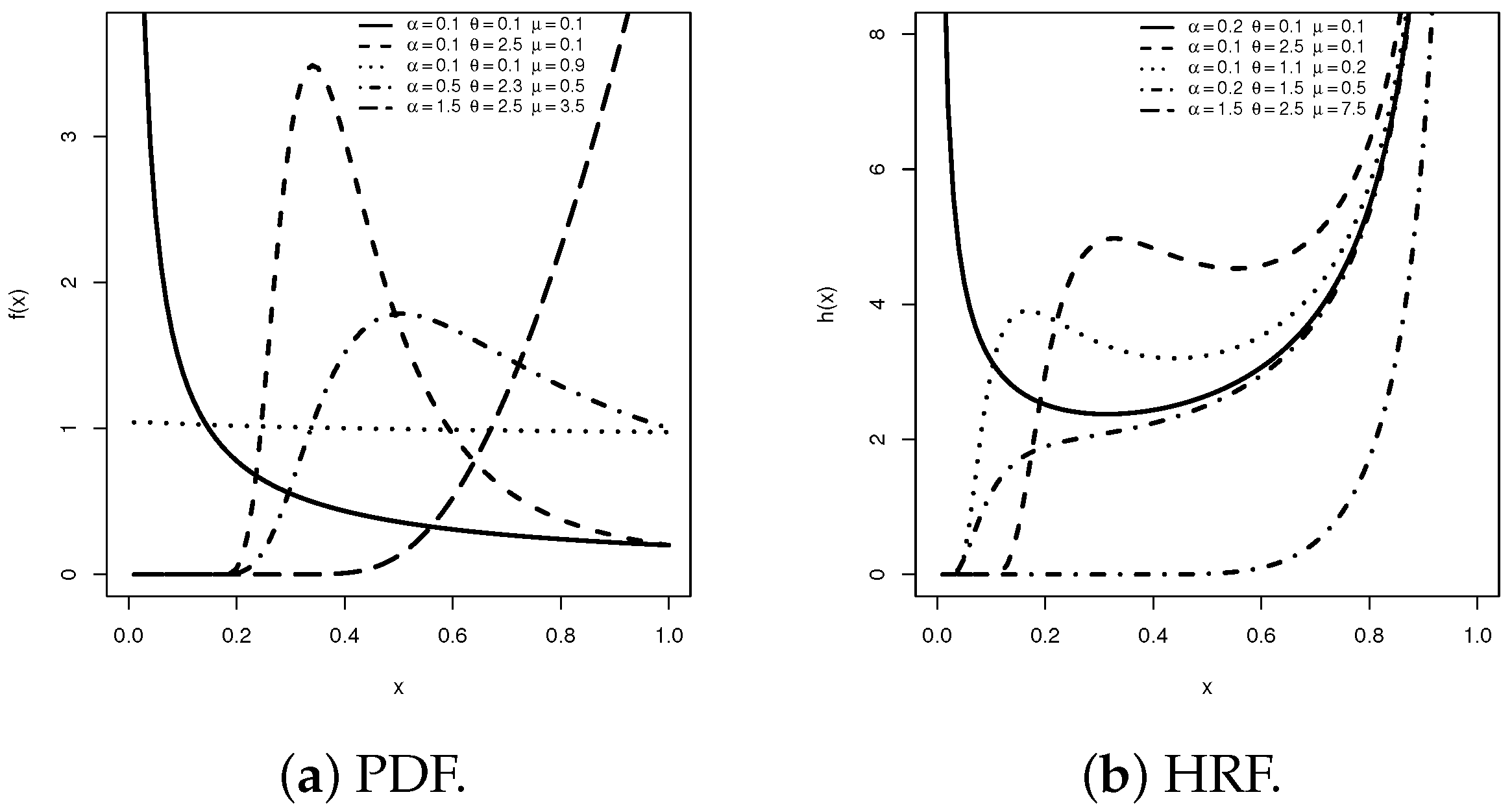
Depending on the parameter values of UGM ( Λ ) , each subplot in Figure 1 displays five density (failure rate) curves illustrating diverse shapes over ( 0 , 1 ) , which reveal the following:
  • Figure 1a shows that the UGM density can be decreasing, increasing, unimodal, or right-skewed. This highlights the distribution’s flexibility in modeling various behaviors, including early risk, balanced variability, and increasing hazard.
  • Figure 1b captures different failure behaviors of the UGM distribution, including decreasing, increasing, bathtub-shaped, and increasing-then-bathtub-shaped hazard rates. These failure rate patterns emphasize the flexibility of the UGM distribution in representing diverse real-world risks.
Figure 1. Several shapes of the UGM density and hazard (failure) rate functions.
Axioms 14 00775 g001

2.2. Quantile and Quartiles

The quantile function of the UGM distribution is a highly tractable and useful property. By the inverse transform theorem, the quantile function can be obtained by inverting the CDF, F ( x ) , in (3). Specifically, the UGM quantile is determined by solving for x in terms of Q ( p ) as
x p = Q ( p ) = F 1 ( p ; Λ ) , 0 < p < 1 .
From (3) and (7), we have
log ( p ) = x μ α θ x θ 1 ,
and after some algebra manipulation, the UGM’s quantile is given by
x p = exp 1 μ log p + α θ x θ 1 , 0 < p < 1 .
It is clear that there is no closed-form quantile function. To compute the quantile Q ( p ) , solve Equation (9) numerically. For real-world applications, numerical methods or approximations can be employed instead of the conventional algebraic form.

3. Distribution Characteristics

In this section, we present several important characteristics of the UGM distribution, including its quantile function, moments, skewness, kurtosis, mean residual life, and order statistics.

3.1. Moments

The rth moment about zero of the UGM distribution, denoted by M r , is given by
M r = 0 1 x r f ( x ; Λ ) d x ,
where f ( · ) is the PDF of the UGM distribution.
From (4), we can rewrite (10) as follows:
M r = 0 1 ( μ + α x θ ) x r μ 1 e α θ ( x θ 1 ) d x .
Substituting the following expansion
e α θ x θ = j = 0 ( α ) j j ! θ j x j θ
into Equation (11), we have
M r = e α θ j = 0 ( α ) j j ! θ j 0 1 x r μ j θ 1 ( μ + α x θ ) d x ,
After simplifying Equation (13), the rth moment of the random variable X can be represented as
M r = e α θ j = 0 ( α ) j j ! θ j μ r μ j θ + 1 + α r μ θ ( j + 1 ) + 1 .
Using r = 1 in Equation (14), the mean of the UGM distribution (say, M * M 1 ) is
M * = e α θ j = 0 ( α ) j j ! θ j μ μ j θ + 1 + α μ θ ( j + 1 ) + 1 .
The variance of the UGM distribution (say, V ) can be calculated as V = M * * ( M * ) 2 , where
M * * = e α θ j = 0 ( α ) j j ! θ j μ μ j θ + 2 + α μ θ ( j + 1 ) + 2 .
An exact closed-form expression of Equation (14) is not available; therefore, numerical methods are required to evaluate the desired moments. Specifically, by setting α = θ { 0.1 , 0.5 , 1.5 } and considering several choices for μ , Table 1 illustrates the behavior of the mean ( M * ), variance ( V ), index of dispersion ( ID ), coefficient of variation ( CV ), skewness ( S ), and kurtosis ( K ) for the UGM model. This assumption uses selected UGM parameter values as representative cases, without loss of generality, to evaluate the behavior of the proposed statistical measures. The following observations can be made:
  • As α increases (for fixed θ and μ ), the values of M * and K increase, whereas V , ID , CV , and S decrease. Similar patterns are observed as μ increases.
  • As θ increases (for fixed α and μ ), the values of M * and S increase, whereas V , ID , CV , and K decrease.
  • The values of S indicate that the distribution can shift from positively skewed (right-skewed) at small parameter values to negatively skewed (left-skewed) as μ increases. Larger θ values tend to reduce the magnitude of skewness, making the distribution more symmetric.
  • The values of K are generally greater than 3, indicating leptokurtic behavior (more peaked with heavier tails than the normal distribution). However, as θ or μ increases, kurtosis tends to decrease, approaching a mesokurtic (normal-like) shape.
  • In short, small μ produces highly skewed and peaked distributions, while larger μ or θ yields more symmetric and less peaked shapes.
  • The UGM data exhibit consistent under-dispersion ( ID < 1 ) across all parameter settings, with the strongest under-dispersion occurring at larger α , θ , and μ values. No over-dispersion is observed in any case.
Table 1. Statistics of the UGM distribution.
α θ μ 0.10.51.5
M V ID CV S K M V ID CV S K M V ID CV S K
0.10.10.1680.0650.3861.5181.5884.5120.1970.0640.3231.2801.4084.0900.3030.0470.1570.7191.2763.906
0.50.3740.0920.2450.8090.4241.9470.3880.0870.2250.7620.4111.9740.4380.0680.1550.5940.4932.076
1.00.5240.0810.1550.543−0.1041.8710.5300.0780.1480.528−0.0961.8770.5520.0660.1200.467−0.0061.834
1.50.6160.0660.1070.416−0.4022.1500.6190.0640.1040.410−0.3922.1400.6300.0580.0920.382−0.3202.038
2.50.7220.0440.0600.289−0.7612.8330.7230.0430.0590.287−0.7542.8170.7270.0410.0560.278−0.7102.703
0.50.10.3840.0890.2310.7760.4051.9600.4330.0730.1690.6240.3732.0280.5260.0470.0890.4110.3752.150
0.50.5050.0820.1620.566−0.0261.8500.5320.0700.1320.499−0.0041.8810.5900.0480.0820.3720.0751.946
1.00.6030.0670.1120.430−0.3482.0870.6170.0610.0980.399−0.3142.0650.6520.0450.0690.326−0.2072.009
1.50.6680.0550.0820.350−0.5662.4150.6770.0510.0750.333−0.5332.3690.6980.0400.0580.287−0.4212.220
2.50.7510.0370.0490.257−0.8573.0890.7540.0350.0470.250−0.8313.0250.7640.0310.0400.229−0.7322.782
1.50.10.6240.0620.0990.399−0.3892.1480.6530.0490.0760.340−0.3372.1390.7040.0310.0440.251−0.2312.129
0.50.6720.0530.0790.342−0.5562.4060.6920.0440.0630.303−0.4972.3480.7310.0290.0400.235−0.3692.241
1.00.7180.0440.0610.291−0.7192.7420.7310.0380.0510.265−0.6582.6400.7590.0270.0350.216−0.5172.430
1.50.7520.0360.0480.254−0.8473.0690.7610.0320.0420.236−0.7882.9390.7820.0240.0310.199−0.6432.649
2.50.8010.0260.0330.202−1.0383.6620.8060.0240.0300.192−0.9863.5060.8180.0190.0210.171−0.8493.121
Keep in mind that Figure 1a illustrates that the PDF of the proposed model can have at most one mode. To formally establish this property, we present the following result, which summarizes these findings and their implications. First, we maximize log ( f ( x ) ) by taking its first derivative, setting it equal to zero, and solving for x to determine the mode, as follows:
( μ 1 ) + α e θ ln ( x ) α θ e θ ln ( x ) μ + α e θ ln ( x ) = 0 .
Since no closed-form expression is available, the mode must be evaluated numerically. To illustrate its behavior, several representative values of θ , α , and μ are considered.

3.2. Mean Residual Life

The mean residual life (MRL) function of the UGM distribution at time t ( 0 , 1 ) , denoted by m ( t ) , is given by
m ( t ) = E [ X t X > t ]
                                                  = 1 R ( t ; Λ ) t 1 ( x t ) f ( x ; Λ ) d x .
Substituting (4) into (17), we get
m ( t ) = 1 R ( t ; Λ ) t 1 e α θ ( x θ 1 ) x μ μ + α x θ d x t 1 t d x ,
Using (12), we can rewrite (19) as
m ( t ) = 1 R ( t ; Λ ) j = 0 ( α ) j e α θ j ! θ j t 1 μ x μ j θ d x + t 1 α x μ θ ( j + 1 ) d x t 1 t d x .
After various simplifications, the MRL of the UGM model is given by
m ( t ) = 1 R ( t ; Λ ) j = 0 ( α ) j e α θ j ! θ j μ 1 t μ j θ + 1 μ j θ + 1 + α 1 t μ θ ( j + 1 ) + 1 μ θ ( j + 1 ) + 1 t ( 1 t ) .

3.3. Moment-Generating Function

The moment-generating function (MGF) of the UGM distribution, denoted by M X ( t ) , is given by
M X ( t ) = 0 1 e t x f ( x ; Λ ) d x .
From (4), the MGF M X ( t ) becomes
M X ( t ) = 0 1 e t x α θ ( x θ 1 ) x μ 1 μ + α x θ d x .
Taking e t x = i = 0 ( t x ) i i ! and (12), Equation (23) can be rewritten as
M X ( t ) = Ω μ 0 1 x μ j θ + i 1 d x + α 0 1 x μ θ ( j + 1 ) + i 1 d x ,
where Ω = i = 0 j = 0 ( α ) j t i e α θ i ! j ! θ j .
As a result, the MGF of the UGM is given by
M X ( t ) = Ω μ μ j θ + i α μ θ ( j + 1 ) + i .

3.4. Order Statistics

Let X ( 1 ) , X ( 2 ) , ... , X ( n ) denote the order statistics from a sample of size n drawn from the UGM population, whose CDF and PDF are given by (3) and (4), respectively. The PDF of the ith order statistic can be expressed as
f x ( i ) ( x ) = a = 0 n i C a f ( x ) [ F ( x ) ] a + i 1 ,
where C a = ( 1 ) a n i a β ( i , n i + 1 ) and β ( · , · ) is the beta function. From (3) and (4), we may write f x ( i ) ( x ) as
f x ( i ) ( x ) = a = 0 n i C a ( μ + a x θ ) x ( μ 1 ) + μ ( a + i 1 ) e a θ ( x θ 1 ) ( a + i ) .
Additionally, the CDF for the ith order statistic is represented as
F x ( i ) ( x ) = a = i n n a [ F ( x ) ] a [ 1 F ( x ) ] n a .
Using (3), we can write F x ( i ) ( x ) as
F x ( i ) ( x ) = a = i n n a x μ e a θ ( x θ 1 ) a 1 x μ e a θ ( x θ 1 ) n a ,
and after simplification, we have
F x ( i ) ( x ) = a = i n j = 0 n a ( 1 ) j n a n a j x μ ( a + j ) e a ( a + j ) θ ( x θ 1 ) .

4. Methods of Estimation

Comparing estimation strategies is essential for identifying the methods that provide the most accurate parameter estimators from a statistical perspective. In this section, we employ eight classical estimation approaches to obtain point estimators of the unknown parameters α , θ , and μ . For a comprehensive discussion of various classical estimation methods, see, for example, Hassan and Alharbi [20], Shafiq et al. [21], and Alqasem et al. [22], among others.

4.1. Maximum Likelihood

The maximum likelihood estimation (MLE) method is the most widely used approach in statistical inference due to its straightforward and intuitive motivation. Moreover, the MLE possesses several desirable properties (see, for example, Rohde [23]). Let x = ( x 1 , x 2 , , x n ) be a random sample. From (4), the log-likelihood function, l ( x | Λ ) = i = 1 n log f ( x | Λ ) , for the UGM distribution can be written as follows:
l ( x | Λ ) i = 1 n log μ + α x i θ + μ i = 1 n log ( x i ) α θ i = 1 n x i θ 1 .
The MLEs ( α ^ M L E , θ ^ M L E , μ ^ M L E ) of ( α , θ , μ ) can be obtained by solving the following system of score equations:
i = 1 n x i θ μ + α x i θ 1 θ i = 1 n x i θ 1 ( α ^ M L E , θ ^ M L E , μ ^ M L E ) = 0 ,
i = 1 n α log ( x i ) x i θ μ + α x i θ + α θ 2 i = 1 n x i θ 1 α θ i = 1 n log ( x i ) x i θ ( α ^ M L E , θ ^ M L E , μ ^ M L E ) = 0 ,
and
i = 1 n 1 μ + α x i θ + i = 1 n log x i ( α ^ M L E , θ ^ M L E , μ ^ M L E ) = 0 ,
respectively. Since Equations (32)–(34) do not admit closed-form solutions, we recommend using numerical optimization methods, such as Newton–Raphson or BFGS, via the maxLik package [24] to obtain ( μ ^ M L E , α ^ M L E , θ ^ M L E ) .

4.2. Maximum Product of Spacings

The maximum product of spacing (MPS) estimation method is widely regarded as a competitive alternative to the MLE in the statistical literature. The MPS estimators (MPSEs) possess many of the same desirable properties as MLEs. Following Cheng and Amin [25], the natural logarithm of the MPS function, to be maximized, is defined as follows when x 1 < x 2 < < x n are the order statistics of a random sample of size n drawn from the UGM population:
P ( Λ ) = i = 1 n + 1 log N i ( Λ ) ,
where N i ( Λ ) = x i μ exp α θ e x i θ 1 x i 1 μ exp α θ e x i 1 θ 1 .
The MPSEs of α , θ , and μ , denoted by α ^ MPS , θ ^ MPS , and μ ^ MPS , can be obtained by simultaneously solving the following three non-linear equations:
P ( Λ ) α = 1 θ i = 1 n + 1 ( 1 e x i θ ) N i 1 ( Λ ) ( 1 e x i 1 θ ) N i 0 ( Λ ) N i ( Λ ) ,
P ( Λ ) μ = i = 1 n + 1 log ( x i ) N i 1 ( Λ ) log ( x i 1 ) N i 0 ( Λ ) N i ( Λ ) ,
and
P ( Λ ) θ = i = 1 n + 1 N i 1 ( Λ ) N i 2 ( Λ ) N i 0 ( Λ ) N i 3 ( Λ ) N i ( Λ ) ,
respectively, where
  • N i 0 ( Λ ) = x i 1 μ exp α θ e x i 1 θ 1 ,
  • N i 1 ( Λ ) = x i μ exp α θ e x i θ 1 ,
  • N i 2 ( Λ ) = α θ 2 e x i θ 1 + α e x i θ x i θ log ( x i ) ,
  • and
  • N i 3 ( Λ ) = α θ 2 e x i 1 θ 1 + α e x i 1 θ x i 1 θ log ( x i 1 ) .
Again, just like in the case of the MLEs, we recommend using the maxLik package (Henningsen and Toomet [24]) to obtain the MPSEs α ^ M P S , μ ^ M P S , and θ ^ M P S for α , θ , and μ , respectively.

4.3. Cramér–Von-Mises

The Cramér–von Mises estimators (CRVMEs) for α , θ , and μ of the UGM distribution, denoted by α ^ C R V M E , θ ^ C R V M E , and μ ^ C R V M E , can be obtained by minimizing the following objective function:
C R ( Λ | x ) = 1 12 n i = 1 n x i μ e ψ i 2 i 1 2 n .
The CRVMEs α ^ C R V M E , θ ^ C R V M E , and μ ^ C R V M E of α , θ , and μ can be obtained by solving the following system of non-linear equations:
C R ( Λ | x ) α = 1 12 n i = 1 n x i μ ( x i θ 1 ) e ψ i ,
C R ( Λ | x ) θ = α θ 2 i = 1 n ( x i θ 1 ) α θ x i θ log ( x i ) ,
and
C R ( Λ | x ) μ = 1 12 n i = 1 n x i μ log ( μ ) e ψ i ,
respectively, where ψ i = α θ ( x i θ 1 ) .

4.4. Weighted Least Squares and Ordinary Least Squares

In this subsection, we examine the weighted-least-squares estimator (WLSE) and ordinary-least-squares estimator (OLSE) of the UGM distribution parameters α , θ , and μ . The goal of these methods is to minimize the squared discrepancies between the theoretical and empirical CDFs. It is known, for the ordered sample x 1 < x 2 < < x n , that F ( Λ | x ) B e t a ( i , n i + 1 ) . As a result, we have
E [ F ( Λ | x ) ] = i n + 1 and V [ F ( Λ | x ) ] = i ( n + 1 i ) ( n + 1 ) 2 ( n + 2 ) .
The OLSEs and WLSEs of the parameters α , θ , and μ can be obtained by minimizing the functions below:
O L ( Λ | x ) = i = 1 n x i μ e ψ i E [ F ( x i ; Λ ) ] ,
and
W L ( Λ | x ) = i = 1 n 1 V [ F ( x i ; Λ ) ] x i μ e ψ i E [ F ( x i ; Λ ) ] 2 ,
with regard to α , θ , and μ .
The OLSEs, denoted by α ^ O L S E , θ ^ O L S E , and μ ^ O L S E , can be obtained by solving the following system of equations simultaneously:
O L ( Λ | x ) α = i = 1 n x i μ e ψ i E [ F ( x i ; Λ ) ] ( x i θ 1 1 ) e ψ i ,
O L ( Λ | x ) θ = α θ 2 i = 1 n x i μ e ψ i E [ F ( x i ; Λ ) ] x i μ x i θ θ 2 x i θ 1 1 e ψ i
and
O L ( Λ | x ) μ = μ i = 1 n μ x i μ e ψ i E [ F ( x i ; Λ ) ] x i μ 1 e ψ i .
Similarly, the WLSEs, denoted by α ^ W L S E , θ ^ W L S E , and μ ^ W L S E , can be obtained by solving the following system of equations simultaneously:
W L ( Λ | x ) α = i = 1 n 1 V [ F ( x i ; Λ ) ] x i μ e ψ i E [ F ( x i ; Λ ) ] ( x i θ 1 1 ) e ψ i ,
W L ( Λ | x ) θ = i = 1 n α μ x i μ θ 2 V [ F ( x i ; Λ ) ] x i μ e ψ i E [ F ( x i ; Λ ) ] ( x i θ θ 2 x i θ 1 1 )
and
W L ( Λ | x ) μ = i = 1 n μ V [ F ( x i ; Λ ) ] x i μ e ψ i E [ F ( x i ; Λ ) ] x i μ 1 e ψ i .

4.5. Percentile

The UGM distribution has a closed-form quantile function, which can be used to estimate percentiles of the unknown parameters. This method aims to minimize the discrepancy between population and sample percentiles. The percentile estimators (PCEs) of α , θ , and μ , denoted by α ^ P C E , θ ^ P C E , and μ ^ P C E , can be obtained for the UGM distribution by minimizing the following objective function:
P ( Λ | x ) = i = 1 n F ( x p i ; Λ ) p i 2 ,
                          = i = 1 n x p i μ e α θ ( x p i θ 1 ) p i 2 .
Since the UGM percentiles do not have a closed-form expression, numerical methods must be employed to obtain α ^ P C E , θ ^ P C E , and μ ^ P C E for the parameters α , θ , and μ , respectively.

4.6. Anderson–Darling and Right-Tail Anderson–Darling

The Anderson–Darling estimators (ADEs) of α , θ , and μ , denoted by α ^ ADE , θ ^ ADE , and μ ^ ADE , can be obtained by minimizing the following function with respect to α , θ , and μ :
A D ( Λ | x ) = n 1 n i = 1 n ( 2 i 1 ) log F ( x i ; Λ ) + log R ( x n i + 1 ; Λ ) .
As a result, the estimators α ^ A D E , θ ^ A D E , and μ ^ A D E of α , θ , and μ , respectively, can be calculated by solving the following equations:
A D ( Λ | x ) α = 1 n θ i = 1 n ( 2 i 1 ) x i μ ( 1 x i θ ) e ψ i F ( x i ; Λ ) + x n i + 1 μ ( 1 x n i + 1 θ ) e ψ i R ( x n i + 1 ; Λ ) ,
A D ( Λ | x ) θ = α n θ 2 i = 1 n ( 2 i 1 ) x i μ A i θ e ψ i F ( x i ; Λ ) + x n i + 1 μ A n i + 1 θ e ψ i R ( x n i + 1 ; Λ ) ,
and
A D ( Λ | x ) μ = μ n i = 1 n ( 2 i 1 ) x i μ 1 e ψ i F ( x i ; Λ ) + x n i + 1 μ 1 e ψ i R ( x n i + 1 ; Λ ) ,
respectively, where ψ i = α θ ( x n i + 1 θ 1 ) and A i θ = 1 x i θ 1 θ 2 x i 1 .
The right-tail Anderson–Darling estimators (RADEs) for the parameters α , θ , and μ , denoted by α ^ RADE , θ ^ RADE , and μ ^ RADE , can be obtained by minimizing the following function:
R A D ( Λ | x ) = n 2 2 i = 1 n F ( x i ; Λ ) i = 1 n ( 2 i 1 ) log R ( x n i + 1 ; Λ ) .
The RADEs α ^ RADE , μ ^ RADE , and θ ^ RADE for the UGM parameters α , θ , and μ can be obtained by solving the following system of non-linear equations:
R A D ( Λ | x ) α = 2 i = 1 n x i μ ( 1 x i θ ) e ψ i 1 n i = 1 n ( 2 i 1 ) x n i + 1 μ ( 1 x n i + 1 θ ) e ψ i R ( x n i + 1 ; Λ ) ,
R A D ( Λ | x ) θ = 2 α θ 2 i = 1 n x i μ θ 2 x i θ 1 + x i θ 1 e ψ i + α n θ 2 i = 1 n ( 2 i 1 ) x n i + 1 μ θ 2 x n i + 1 θ 1 + x n i + 1 θ 1 e ψ i R ( x n i + 1 ; Λ ) ,
and
R A D ( Λ | x ) μ = 2 μ i = 1 n x i μ 1 e ψ i μ n i = 1 n ( 2 i 1 ) x n i + 1 μ 1 e ψ i R ( x n i + 1 ; Λ ) ,
respectively.

5. Simulation Study

This section utilizes a Monte Carlo simulation framework to investigate the behavior of the proposed estimators under various controlled conditions. To this end, a total of 5000 synthetic datasets are generated for each considered scenario, with sample sizes n (=20, 50, 100, 150, 200). The data are drawn from the UGM ( Λ ) distribution, incorporating different configurations of the model parameters to capture a range of distributional shapes. In particular, we examine the impact of two values of each unknown parameter, such as α ( = 0.8 , 1.8 ) , θ ( = 0.5 , 1.5 ) , and μ ( = 0.2 , 1.2 ) , applied across the following five parameter combinations for Λ :
  • Set-1: ( 0.8 , 0.5 , 0.2 ) ;
  • Set-2: ( 1.8 , 1.5 , 1.2 ) ;
  • Set-3: ( 0.8 , 1.5 , 1.2 ) ;
  • Set-4: ( 1.8 , 1.5 , 0.2 ) ;
  • Set-5: ( 1.8 , 0.5 , 1.2 ) .
All computational analyses were carried out using the R (v 4.2.2) software environment. The parameter values α , θ , and μ were chosen to encompass a wide range of distributional shapes of the UGM model. In particular, smaller values of ( α , θ , μ ) generate highly skewed and heavy-tailed distributions, whereas larger values yield more symmetric and lighter-tailed forms. This selection allows the simulation study to evaluate estimator performance under both extreme and moderate scenarios, thereby providing a comprehensive assessment of robustness and accuracy. It is worth noting that the starting points of α , θ , and μ were set to their true values. Alternatively, moment-based or percentile-based initialization, together with grid-search refinement, can be used to assign suitable starting points for each parameter.
A comparative evaluation of all estimation procedures was conducted using three standard error metrics: mean squared error (MSE), mean absolute bias (MAB), and relative absolute bias (RAB). For each method evaluated, the estimates for these metrics, along with total ranks (TRs) and order ranks (ORs) for α , θ , and μ , are presented in Table 2, Table 3, Table 4, Table 5 and Table 6. Across all experimental conditions, results show a clear trend of improved estimator accuracy with larger sample sizes n, confirming the consistency of the estimators for all parameters. Notably, both ML and MPS methods consistently provide more accurate and stable estimates compared to other approaches.
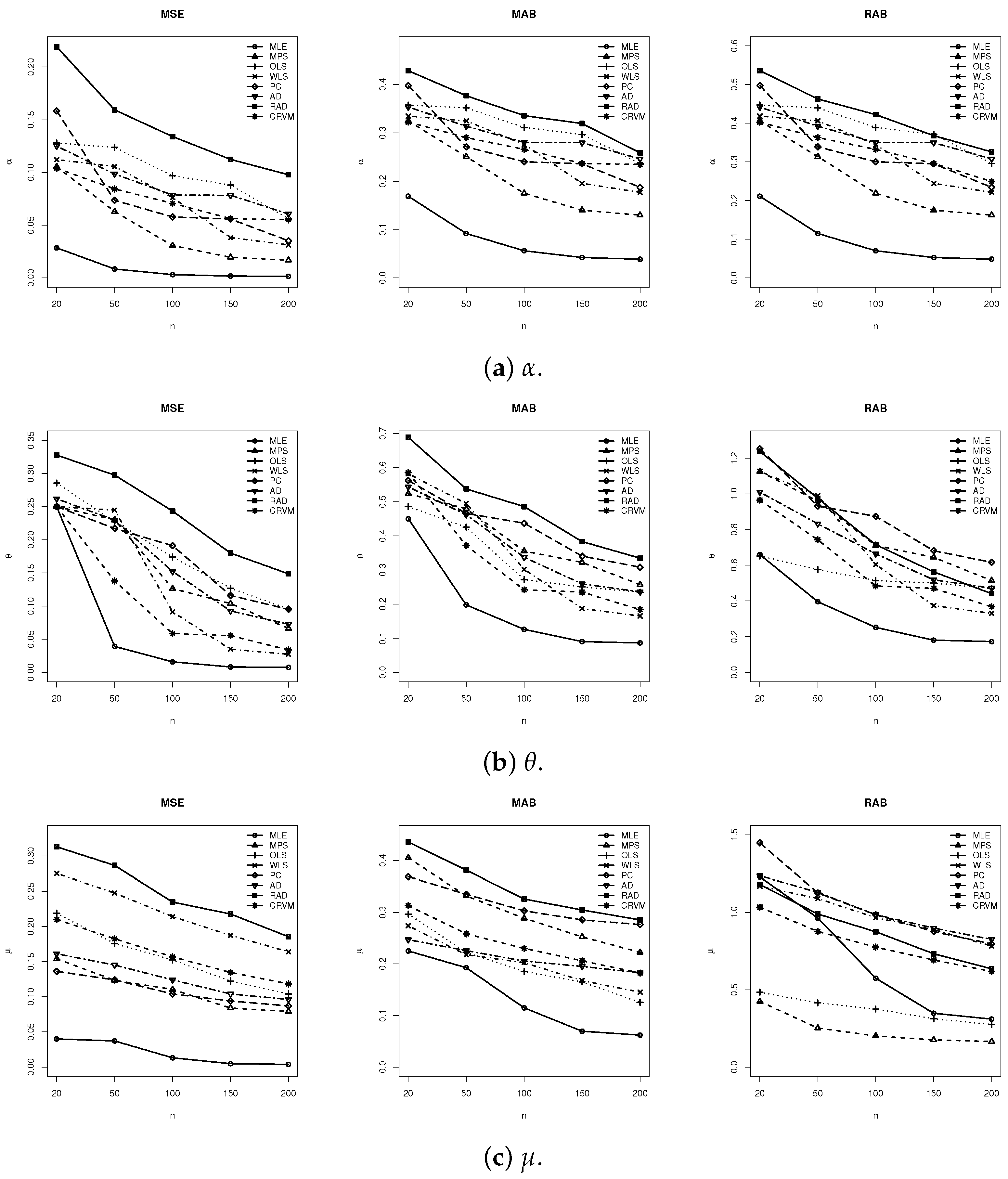
To summarize overall performance across different parameter settings, mean total ranks (MTRs) and mean order ranks (MORs) were calculated and are summarized in Table 7. This table demonstrates that the MLE generally outperforms all others in most scenarios, with the MPSE ranking close behind. When ranking the estimation strategies according to their average performance, the efficiency from most to least effective is as follows: MLE, MPSE, CRVME, OLSE, WLSE, PCE, ADE, and RADE. These rankings are fully aligned with the individual results presented in Table 2, Table 3, Table 4, Table 5 and Table 6. From Set-1 (as an example), Figure 2 displays the simulated results, including MSE, MAB, and RAB values corresponding to the parameters α , θ , and μ . The fitted lines shown in Figure 2 correspond to the estimation methods and confirm the same inferential findings listed in Table 2.
To summarize, we recommend using the ML method as the preferred approach in practical applications involving the UGM distribution, with the MPS method serving as a reliable alternative when ML is unsuitable or computationally intensive.

6. Real-World Applications

This section examines two distinct engineering applications to demonstrate the practical utility of the proposed inferential methods and to highlight the advantages of the UGM model in capturing various real-world scenarios. These applications are as follows:
  • Application 1: This application analyzes twelve core samples extracted from petroleum reservoirs, each obtained across four distinct cross sections, resulting in a total of forty-eight observations. For each core sample, permeability was measured as the primary response variable. Additionally, three key geometric properties were recorded at the cross-section level: total pore area, total pore perimeter, and pore shape. These variables are critical for characterizing the microstructural features influencing fluid flow through the reservoir rock and provide a basis for investigating the relationship between pore geometry and permeability. The petroleum reservoirs dataset was first provided by the R Core Team [26] and later reanalyzed by Mazucheli et al. [4] and Dey et al. [7].
  • Application 2: This application investigates twenty mechanical components by analyzing their time to failure under controlled operational stress, aiming to quantify their reliability characteristics, estimate distributional parameters, and provide predictive insights into failure risk. Given that this dataset contains a single extreme outlier (0.485), the analysis is presented as an illustrative case study without loss of generality. Accordingly, the results are intended to demonstrate the potential applicability of the UGM distribution in small-sample contexts. The mechanical components dataset was presented by Murthy et al. [27] and later discussed by Elshahhat et al. [28] and Alqasem et al. [22].
For clarification, in Application 1, the UGM distribution captures a non-monotonic hazard rate consistent with systems that exhibit early failures followed by stability, which is a feature not accounted for by competing bounded models. In Application 2, the fitted UGM parameters indicate heavier tails, underscoring the non-negligible probabilities of extreme performance outcomes and their implications for reliability margins.
Before analyzing the new UGM model and after multiplying each data point in the petroleum reservoirs dataset by two, Table 8 lists the time data points for Applications 1 and 2. It should be noted that the permeability data were rescaled to the unit interval (by multiplication with a constant) solely for compatibility with bounded distributions and for computational convenience; this transformation does not alter the substantive interpretation of the results. Furthermore, Table 9 presents a comprehensive summary of descriptive statistics—including the mean, mode, three quartiles ( Q i , i = 1 , 2 , 3 ), standard deviation (SD), and skewness—for the datasets used in Applications 1 and 2. The summary statistics reveal that Application 1 employed a dataset with a relatively balanced distribution and modest right skew, whereas Application 2 used a dataset with heavy right skew, indicating the presence of extreme upper values. The greater spread and higher mean in Application 1’s data also reflect more variability and generally larger observations compared to the more compact and lower-valued data in Application 2.
To evaluate the performance of the UGM distribution across the full datasets presented in Applications 1 and 2, we compared it against nine alternative lifetime models characterized by flexible and unbounded failure rate structures (see Table 10). The model comparison was conducted using eight widely used goodness-of-fit and information criteria: (i) negative log-likelihood ( LL ), (ii) Akaike Information ( AI ), (iii) Bayesian Information ( BI ), (iv) Consistent AI ( CAI ), (v) Hannan–Quinn Information ( HQI ), (vi) Anderson–Darling ( AD ), (vii) Cramér–von Mises ( CvM ), and (viii) Kolmogorov–Smirnov ( KS ) statistic along with its corresponding P -value.
Using the AdequacyModel package (Marinho et al. [29]), the detailed results of criteria (i)–(viii) are summarized in Table 11. In addition to model selection metrics, Table 12 provides the MLEs (along with standard errors, SEs) of each model parameter. Here, we initialize all parameters with starting points chosen based on their theoretical domains; see, for example, Mariel et al. [30]. According to the estimated selection criteria, the best (optimal) models correspond to the smallest values of LL , AI , BI , CAI , HQI , AD , CvM , and KS and of the largest P -value. The findings in Table 11 clearly favor the proposed UGM model as the most suitable candidate among all competing alternatives presented in Table 10.
Table 10. Nine competitive models for UGM distribution.
ModelSymbolAuthor(s)
Complementary unit-WeibullCUW ( α , θ , μ ) Guerra et al. [10]
Unit-Birnbaum–SaundersUBS ( θ , μ ) Mazucheli et al. [6]
Unit-log–logULL ( θ , μ ) Korkmaz and Korkmaz [12]
Topp–LeoneTL ( μ ) Topp and Leone [31]
Unit-WeibullUW ( θ , μ ) Mazucheli et al. [4]
Unit-GammaUG ( θ , μ ) Dey et al. [7]
Unit-GompertzUGo ( θ , μ ) Mazucheli et al. [8]
KumaraswamyKum ( θ , μ ) Kumaraswamy [3]
BetaBeta ( θ , μ ) Gupta and Nadarajah [1]
Table 11. Summary fit for the UGM and its competitor models.
Model LL AI BI CAI HQI AD CvM KS
Distance P -value
Application 1
UGM−25.499−44.998−39.384−44.452−42.8760.2440.0350.0850.880
CUW−12.564−21.129−17.386−20.862−19.7142.4100.3910.1620.163
UBS−7.3930−10.786−7.0436−10.519−9.37173.3840.5640.2300.012
ULL−24.886−43.772−38.030−44.206−41.3580.3980.0590.1050.666
TL−13.872−25.743−23.872−25.656−25.0361.5280.2440.2180.021
UW−23.196−42.392−38.650−42.126−40.9780.6830.1080.1300.387
UG−18.046−32.092−28.350−31.826−30.6780.7880.1280.1740.109
UGo−25.387−44.774−39.031−44.151−40.9450.2460.0380.0890.876
Kum−15.924−27.848−24.106−27.582−26.4341.9260.3100.1750.104
Beta−17.622−31.245−27.502−30.978−29.8301.6660.2670.1760.102
Application 2
UGM−38.048−70.097−67.110−68.597−69.5140.3420.0460.1670.633
CUW−24.950−45.900−43.909−45.194−45.5122.7440.4560.2800.088
UBS−26.103−48.205−46.214−47.499−47.8172.6720.4410.2760.094
ULL−37.808−69.617−66.625−67.911−71.2280.5170.0660.1720.620
TL−13.743−25.486−24.490−25.264−25.2912.1560.3390.4840.038
UW−35.819−67.637−65.645−66.931−67.2480.8260.1080.1720.624
UG−29.272−54.544−52.553−53.839−54.1561.5790.2320.2150.314
UGo−8.3496−12.699−10.708−11.993−12.3102.0780.3240.5110.035
Kum−25.648−47.297−45.305−46.591−46.9082.6500.4370.2630.126
Beta−27.881−51.763−49.771−51.057−51.3742.3150.3700.2540.152
Table 12. The fitted parameters of UGM and its competitor models.
ModelMLE
α θ μ
Est.SEEst.SEEst.SE
Application 1
UGM0.23880.19012.42410.67190.12450.2833
CUW--1.60670.15680.44180.0343
UBS--0.67270.06870.72220.0662
ULL--1.98570.23361.92580.1392
TL----2.20620.3184
UW--1.00350.15082.69840.3202
UG--4.06980.79904.55160.9511
UGo--0.06370.03162.68470.3755
Kum--2.31290.30054.16710.9699
Beta--3.36130.66134.16430.8311
Application 2
UGM0.00220.00053.04780.14650.01160.0321
CUW--1.41580.19810.11100.0193
UBS--0.28410.04492.14270.1347
ULL--5.97280.90401.00380.0032
TL----0.62480.1397
UW--0.00320.00136.74140.5128
UG--17.6485.52897.91452.5150
UGo--46.85670.90360.00970.0146
Kum--1.58650.244221.80910.172
Beta--3.11290.936921.8267.0425
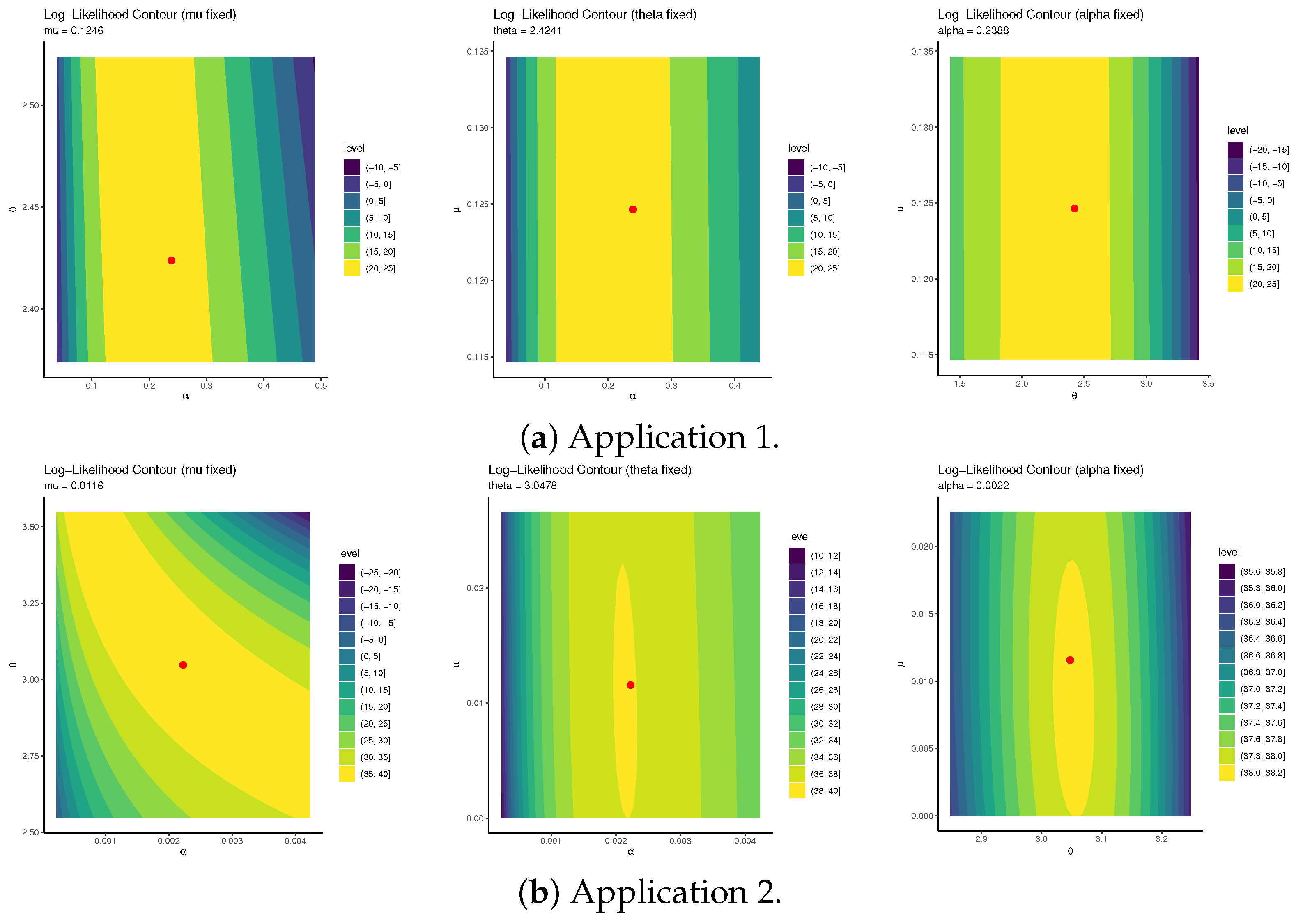
To initialize the parameters α , θ , and μ of the UGM distribution for the proposed computational analysis based on the two real-world datasets in Applications 1 and 2, the contours of the log-likelihood function for these parameters are displayed in Figure 3. It indicates that the optimal starting values (red-point coordinates) of α , θ , and μ are close to their MLEs reported in Table 11. Moreover, the results confirm that the MLEs of α , θ , and μ exist and are unique. Therefore, we recommend using these estimates as initial values for subsequent computational iterations.
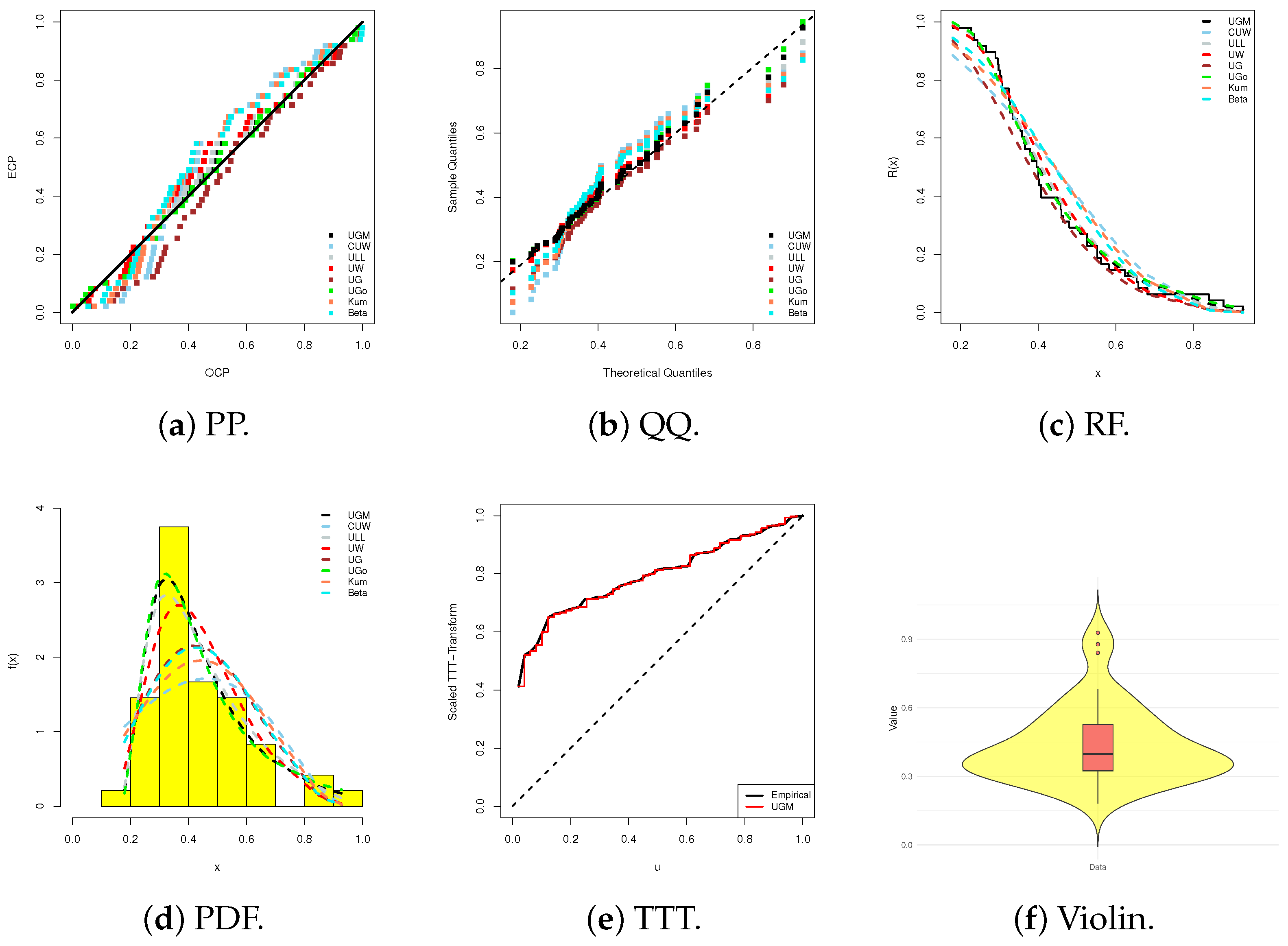
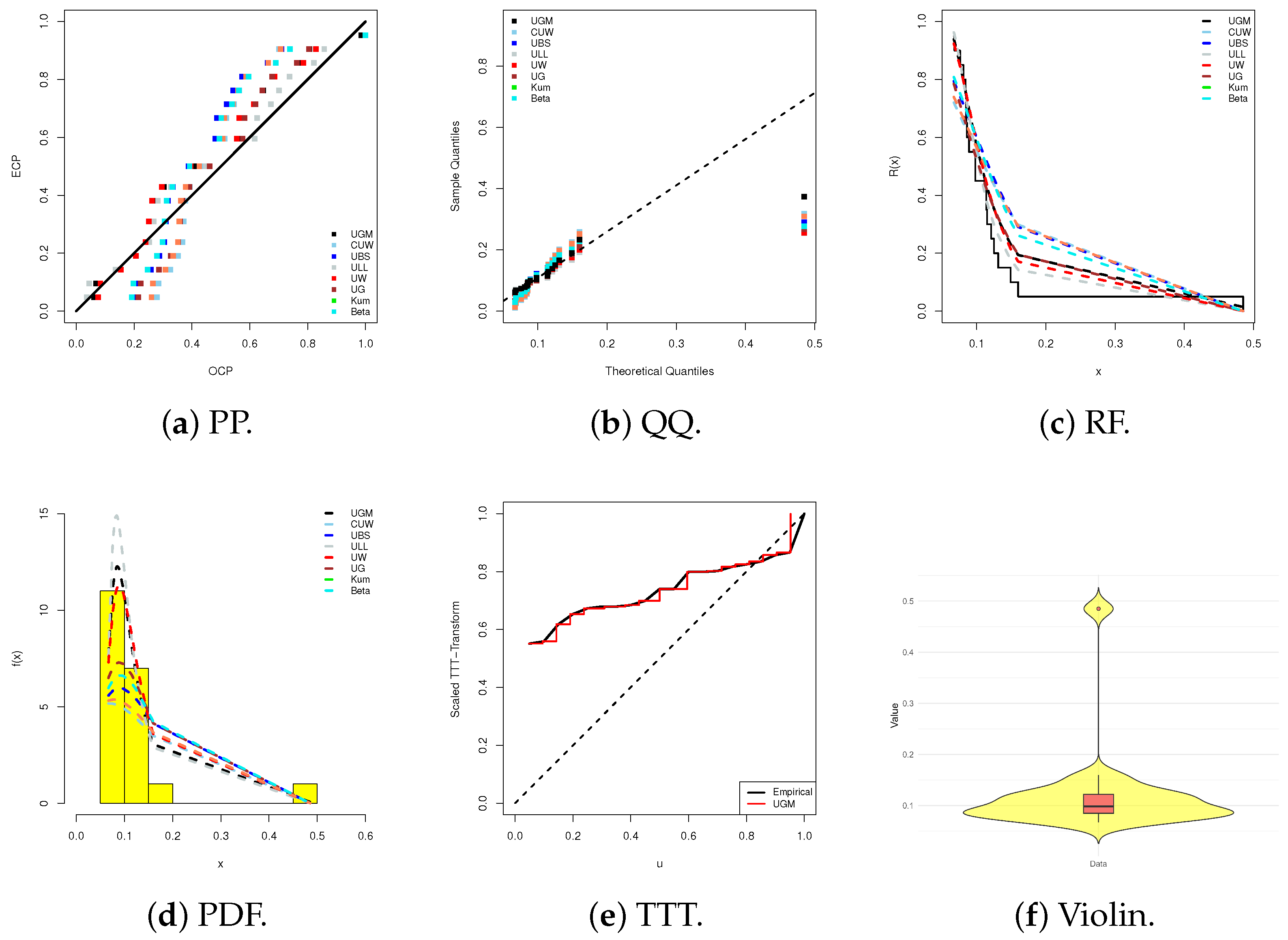
Using six visualization panels for a detailed comparison of the UGM and its competitor models under the datasets analyzed in Applications 1 and 2, Figure 4 and Figure 5 display the following: (i) probability–probability (PP) plots, (ii) quantile–quantile (QQ) plots, (iii) fitted RFs, (iv) fitted PDFs, (v) scale TTT-transform (TTT), and (vi) violin plots with boxplots.
From Figure 4 and Figure 5, the following observations can be made:
  • Subplots (a)–(c) visually support the numerical results in Table 11, clearly showing that the UGM model produces fitted values closely aligned with the empirical observations in both Application 1 and Application 2.
  • Subplot (d) indicates that the fitted UGM density shapes for Applications 1 and 2 are right-skewed and strictly right-skewed, respectively.
  • Subplot (e) shows that the proposed datasets in Applications 1 and 2 exhibit increasing and upside-down bathtub failure rate shapes, respectively, supporting the theoretical UGM failure rates first depicted in Figure 1.
  • Subplot (f) demonstrates that Application 1’s data have a wider spread with a higher median, indicating greater variation, whereas Application 2’s data are more concentrated with a lower median, suggesting more consistency. Overall, Application 1’s dataset appears more heterogeneous, while Application 2’s dataset is more homogeneous.
While several competing models in Table 11 achieve an acceptable fit, the superiority of the UGM distribution is supported by multiple complementary criteria. In particular, the UGM consistently attains the lowest values of all information-based measures while also yielding the highest p -value, indicating an optimal balance between goodness of fit and parsimony. Moreover, graphical diagnostics (Figure 4 and Figure 5) demonstrate a closer agreement between the empirical and theoretical distributions under the UGM model. Beyond these empirical findings, the UGM possesses a theoretical advantage: unlike most unit distributions, it can flexibly accommodate decreasing, increasing, bathtub-shaped, and inverted-bathtub-shaped hazard rate patterns.

7. Conclusions

In this paper, we introduced and studied a novel continuous probability distribution defined on the unit interval ( 0 , 1 ) . The model is constructed by applying a suitable transformation to the classical GM distribution, enabling flexible modeling of bounded data while retaining key characteristics of the parent distribution. We thoroughly investigated its statistical and mathematical properties, including explicit derivations of the cumulative distribution function, probability density function, quantile function, and moments. Important reliability properties, such as the hazard rate, reversed hazard rate, and mean residual life, were also examined, highlighting the model’s potential in survival and reliability analysis. To estimate model parameters, eight estimation methods were considered, including maximum likelihood, maximum product of spacings, and ordinary least squares. A comprehensive simulation study demonstrated that maximum likelihood consistently provides the most accurate and efficient parameter estimates, closely followed by the product of spacings method in terms of bias and mean square error. Applications to real-world datasets further illustrated the model’s superior flexibility and goodness of fit relative to existing bounded distributions, particularly in capturing diverse hazard rate shapes, including decreasing, increasing, bathtub, and inverted-bathtub forms. The results underscore two major insights. First, the distribution offers an unprecedented range of shapes for both its density and hazard functions, which are difficult to replicate with traditional bounded models. Second, maximum likelihood and maximum product of spacings are the most reliable estimation techniques, providing stable and accurate parameter inference. This work opens several avenues for future research. Theoretically, extensions to regression frameworks, multivariate forms, and copula-based constructions could further enhance the model’s applicability. Methodologically, Bayesian estimation procedures and computationally efficient algorithms for large datasets merit further investigation. Practically, the distribution can be especially useful for modeling bounded reliability data in finance, biomedical studies, environmental sciences, and other fields, with potential for incorporating covariate information or dependence structures to improve modeling performance. Overall, the proposed distribution represents a flexible, tractable, and powerful addition to the family of bounded probability models, offering strong potential for both theoretical development and practical application across diverse scientific domains.
Author Contributions

Methodology, R.A., H.R., and A.E.; funding acquisition, R.A.; software, A.E.; supervision, R.A.; writing—original draft, H.R. and A.E.; writing—review and editing, R.A. and H.R. All authors have read and agreed to the published version of the manuscript.

Funding

This research was funded by Princess Nourah bint Abdulrahman University Researchers Supporting Project number (PNURSP2025R50), Princess Nourah bint Abdulrahman University, Riyadh, Saudi Arabia.

Data Availability Statement

The authors confirm that the data supporting the findings of this study are available within the article.

Conflicts of Interest

The authors declare no conflicts of interest.

Appendix A. Derivation Steps of the UGM Distribution

Proposition A1.
If Y G M ( Λ ) with CDF
G ( y ; Λ ) = 1 exp μ y α θ e θ y 1 , y > 0 ,
then the random variable  X = exp ( Y )  has CDF
F ( x ; Λ ) = exp μ ln ( x ) α θ e θ ln ( x ) 1 , 0 < x < 1 .
Proof. 
Since the transformation x = exp ( y ) is strictly decreasing, for 0 < x < 1 , we have
F ( x ) = Pr ( X x ) = Pr e Y x = Pr Y ln ( x ) .
By continuity of Y, this can be expressed as
F ( x ) = 1 G ( ln ( x ) ) .
Substituting the expression for G yields
F ( x ) = 1 1 exp μ ( ln ( x ) ) α θ e θ ( ln ( x ) ) 1 = exp μ ln ( x ) α θ e θ ln ( x ) 1 , 0 < x < 1 ,
which coincides with Equation (3). □
Proposition A2.
Let Y GM ( Λ ) have PDF
g ( y ; Λ ) = ( μ + α e θ y ) exp μ y α θ ( e θ y 1 ) , y > 0 .
If X = e Y , then the PDF of X is
f ( x ; Λ ) = x 1 μ + α x θ exp μ ln ( x ) α θ ( x θ 1 ) , 0 < x < 1 .
Proof. 
With the monotone transformation x = e y , we have the inverse relation y = ln ( x ) and d y d x = 1 x | d y d x | = 1 x , 0 < x < 1 .
Applying the change-of-variable formula for densities,
f X ( x ) = g Y y ( x ) | d y d x | ,
we substitute y = ln ( x ) into g and multiply by | d y / d x | = 1 / x . Using e θ y = e θ ln ( x ) = x θ gives
f ( x ; Λ ) = 1 x μ + α e θ ( ln ( x ) ) exp μ ( ln ( x ) ) α θ e θ ( ln ( x ) ) 1 = x 1 μ + α x θ exp μ ln ( x ) α θ ( x θ 1 ) , 0 < x < 1 ,
which coincides with Equation (4). □

References

  1. Gupta, A.K.; Nadarajah, S. Handbook of Beta Distribution and Its Applications; CRC Press: Boca Raton, FL, USA, 2004. [Google Scholar]
  2. Lai, C.D.; Jones, G. Beta hazard rate distribution and applications. IEEE Trans. Reliab. 2014, 64, 44–50. [Google Scholar] [CrossRef]
  3. Kumaraswamy, P. A generalized probability density function for double-bounded random processes. J. Hydrol. 1980, 46, 79–88. [Google Scholar] [CrossRef]
  4. Mazucheli, J.; Menezes, A.F.B.; Ghitany, M.E. The unit-Weibull distribution and associated inference. J. Appl. Probab. Stat. 2018, 13, 1–22. [Google Scholar]
  5. Menezes, A.F.B.; Mazucheli, J.; Dey, S. The unit-logistic distribution: Different methods of estimation. Pesqui. Oper. 2018, 38, 555–578. [Google Scholar] [CrossRef]
  6. Mazucheli, J.; Menezes, A.F.; Dey, S. The unit-Birnbaum-Saunders distribution with applications. Chil. J. Stat. 2018, 9, 47–57. [Google Scholar]
  7. Dey, S.; Menezes, A.F.; Mazucheli, J. Comparison of estimation methods for unit-gamma distribution. J. Data Sci. 2019, 17, 768–801. [Google Scholar] [CrossRef]
  8. Mazucheli, J.; Menezes, A.F.; Dey, S. Unit-Gompertz distribution with applications. Statistica 2019, 79, 25–43. [Google Scholar]
  9. Mazucheli, J.; Menezes, A.F.B.; Chakraborty, S. On the one parameter unit-Lindley distribution and its associated regression model for proportion data. J. Appl. Stat. 2019, 46, 700–714. [Google Scholar] [CrossRef]
  10. Guerra, R.R.; Peña-Ramírez, F.A.; Bourguignon, M. The unit extended Weibull families of distributions and its applications. J. Appl. Stat. 2021, 48, 3174–3192. [Google Scholar] [CrossRef]
  11. Krishna, A.; Maya, R.; Chesneau, C.; Irshad, M.R. The unit Teissier distribution and its applications. Math. Comput. Appl. 2022, 27, 12. [Google Scholar] [CrossRef]
  12. Korkmaz, M.Ç.; Korkmaz, Z.S. The unit log–log distribution: A new unit distribution with alternative quantile regression modeling and educational measurements applications. J. Appl. Stat. 2023, 50, 889–908. [Google Scholar] [CrossRef] [PubMed]
  13. Karakaya, K.; Rajitha, C.S.; Sağlam, Ş.; Tashk, Y.A.; Bakr, M.E.; Muse, A.H.; Kumar, A.; Hussam, E.; Gemeay, A.M. A new unit distribution: Properties, estimation, and regression analysis. Sci. Rep. 2024, 14, 7214. [Google Scholar] [CrossRef] [PubMed]
  14. Bashiru, S.O.; Kayid, M.; Sayed, R.M.; Balogun, O.S.; Abd El-Raouf, M.M.; Gemeay, A.M. Introducing the unit Zeghdoudi distribution as a novel statistical model for analyzing proportional data. J. Radiat. Res. Appl. Sci. 2025, 18, 101204. [Google Scholar] [CrossRef]
  15. Marshall, A.W.; Olkin, I. Life Distributions; Springer: New York, NY, USA, 2007. [Google Scholar]
  16. Jodrá, P. A closed-form expression for the quantile function of the Gompertz–Makeham distribution. Math. Comput. Simul. 2009, 79, 3069–3075. [Google Scholar] [CrossRef]
  17. Missov, T.I.; Lenart, A. Gompertz–Makeham life expectancies: Expressions and applications. Theor. Popul. Biol. 2013, 90, 29–35. [Google Scholar] [CrossRef] [PubMed]
  18. Wang, J.; Guo, X. The Gompertz model and its applications in microbial growth and bioproduction kinetics: Past, present and future. Biotechnol. Adv. 2024, 72, 108335. [Google Scholar] [CrossRef]
  19. Castellares, F.; Patrício, S.; Lemonte, A.J. On the Gompertz–Makeham law: A useful mortality model to deal with human mortality. Braz. J. Probab. Stat. 2022, 36, 613–639. [Google Scholar] [CrossRef]
  20. Hassan, A.S.; Alharbi, R.S. Different estimation methods for the unit inverse exponentiated Weibull distribution. Commun. Stat. Appl. Methods 2023, 30, 191–213. [Google Scholar] [CrossRef]
  21. Shafiq, A.; Sindhu, T.N.; Dey, S.; Lone, S.A.; Abushal, T.A. Statistical features and estimation methods for half-logistic unit-gompertz type-I model. Mathematics 2023, 11, 1007. [Google Scholar] [CrossRef]
  22. Alqasem, O.A.; Nassar, M.; Abd Elwahab, M.E.; Elshahhat, A. A new inverted Pham distribution for data modeling of mechanical components and diamond in South-West Africa. Phys. Scr. 2024, 99, 115268. [Google Scholar] [CrossRef]
  23. Rohde, C.A. Introductory Statistical Inference with the Likelihood Function; Springer: New York, NY, USA, 2014. [Google Scholar]
  24. Henningsen, A.; Toomet, O. maxLik: A package for maximum likelihood estimation in R. Comput. Stat. 2011, 26, 443–458. [Google Scholar] [CrossRef]
  25. Cheng, R.C.H.; Amin, N.A.K. Estimating parameters in continuous univariate distributions with a shifted origin. J. R. Stat. Soc. Ser. (Methodol.) 1983, 45, 394–403. [Google Scholar] [CrossRef]
  26. R Core Team. Rock: Measurements on Petroleum Rock Samples, Datasets Package, R Software. 2017. Available online: https://stat.ethz.ch/R-manual/R-devel/library/datasets/html/rock.html (accessed on 15 August 2025).
  27. Murthy, D.N.P.; Xie, M.; Jiang, R. Weibull Models; Wiley series in Probability and Statistics; Wiley: Hoboken, NJ, USA, 2004. [Google Scholar]
  28. Elshahhat, A.; El-Sherpieny, E.S.A.; Hassan, A.S. The Pareto–Poisson Distribution: Characteristics, Estimations and Engineering Applications. Sankhya A 2023, 85, 1058–1099. [Google Scholar] [CrossRef]
  29. Marinho, P.R.D.; Silva, R.B.; Bourguignon, M.; Cordeiro, G.M.; Nadarajah, S. dequacyModel: An R package for probability distributions and general purpose optimization. PloS ONE 2019, 14, e0221487. [Google Scholar] [CrossRef] [PubMed]
  30. Mariel, P.; Campbell, D.; Sandorf, E.D.; Meyerhoff, J.; Vega-Bayo, A.; Blevins, R. Maximum Likelihood and Related Issues. In Environmental Valuation with Discrete Choice Experiments in R: A Guide on Design, Implementation, and Data Analysis; Springer Nature: Cham, Switzerland, 2025; pp. 197–224. [Google Scholar]
  31. Topp, C.W.; Leone, F.C. A family of J-shaped frequency functions. J. Am. Stat. Assoc. 1955, 50, 209–219. [Google Scholar] [CrossRef]
Figure 2. Estimation plots of α , θ , and μ .
Axioms 14 00775 g002
Figure 3. Contour maps of α (left), θ (center), and μ (right) from physics and engineering datasets.
Axioms 14 00775 g003
Figure 4. Fitting diagrams of the UGM and its competitor models from Application 1.
Axioms 14 00775 g004
Figure 5. Fitting diagrams of the UGM and its competitor models from Application 2.
Axioms 14 00775 g005
Table 2. The estimates (1st column) and their ranks (2nd column) of α , θ , and μ from Set-1.
nMetricPar.MLEMPSEOLSEWLSEPCSCRVMEADERADE
20MSE α 0.02910.10530.12860.11240.15870.10420.12550.2198
θ 0.25010.25020.28670.25020.25020.25020.26260.3288
μ 0.04010.15430.21960.27570.13620.21050.16140.3138
MAB α 0.16910.32530.35860.33540.39870.32220.35450.4298
θ 0.45010.52430.48620.58260.56250.58570.54440.6898
μ 0.22510.40570.29740.27430.36960.31350.24720.4368
RAB α 0.21110.40630.44760.41940.49870.40320.44250.5368
θ 0.66021.12650.65211.12661.25280.96531.01041.2387
μ 1.22960.42410.48421.17041.44781.03431.23671.1805
TR→ 15 30 40 40 52 31 42 68
OR→ 1 2 4.5 4.5 7 3 6 8
50MSE α 0.00810.06320.12470.10660.07430.08440.09950.1598
θ 0.03910.23060.22740.24570.21730.13820.23050.2988
μ 0.03710.12320.17650.24870.12430.18260.14540.2868
MAB α 0.09210.25120.35270.32560.27130.29140.31450.3778
θ 0.19810.48060.42530.49570.46650.37120.46240.5388
μ 0.19310.33260.22330.21820.33570.25850.22640.3818
RAB α 0.11510.31420.44070.40660.33930.36340.39250.4638
θ 0.39610.95960.57620.98980.93250.74330.83240.9757
μ 0.96440.25210.41521.09061.12570.87731.12980.9905
TR→ 12 33 40 55 39 33 44 68
OR→ 1 2.5 5 7 4 2.5 6 8
100MSE α 0.00310.03120.09770.07650.05830.07140.07960.1348
θ 0.01610.12740.17460.09130.19170.05920.15250.1808
μ 0.01310.11030.15250.21470.10420.15760.12440.2358
MAB α 0.05610.17520.31170.27650.24030.26640.28060.3368
θ 0.12610.35660.27230.30240.43770.24220.33750.4868
μ 0.11510.28960.18520.20330.30370.23050.20640.3268
RAB α 0.07010.21920.38970.34550.30030.33240.35060.4228
θ 0.25210.71160.51430.60440.87480.48420.66450.7157
μ 0.57430.20110.37520.96560.98570.77540.98580.8755
TR→ 11 32 42 42 47 33 49 68
OR→ 1 2 4.5 4.5 6 3 7 8
150MSE α 0.00210.02020.08870.03830.05640.05650.07860.1128
θ 0.00810.10450.12770.03520.11660.05530.09340.1498
μ 0.00510.08420.12250.18770.09430.13560.10440.1858
MAB α 0.04210.14020.29770.19630.23640.23750.28060.3198
θ 0.09010.32270.25040.18720.34180.23530.25950.3836
μ 0.07010.25360.16520.16830.28570.20650.19540.3058
RAB α 0.05310.17520.37170.24530.29540.29650.35060.3688
θ 0.18010.64470.50140.37420.68180.47130.51950.5636
μ 0.34830.17510.31320.88870.87660.69240.89980.7335
TR→ 11 34 45 32 50 39 48 65
OR→ 1 3 5 2 7 4 6 8
200MSE α 0.00210.01720.05660.03130.03540.05550.06170.0988
θ 0.00710.06640.09670.02720.09560.03430.07350.2498
μ 0.00410.07920.10450.16480.08730.11860.09640.1547
MAB α 0.03910.13020.23760.17730.18840.23550.24670.2598
θ 0.08610.25760.23540.16520.30880.18430.23650.3357
μ 0.06210.22360.12520.14530.27670.18240.18350.2858
RAB α 0.04810.16220.29660.22130.23440.24950.30870.3268
θ 0.17210.51470.46950.33020.61680.36830.47260.4414
μ 0.31030.16510.27520.78260.79770.61840.82580.6355
TR→ 11 32 43 32 51 38 54 63
OR→ 1 2.5 5 2.5 6 4 7 8
Table 3. The estimates (1st column) and their ranks (2nd column) of α , θ , and μ from Set-2.
nMetricPar.MLEMPSEOLSEWLSEPCSCRVMEADERADE
20MSE α 0.10211.54151.59561.61971.27521.42731.47042.2378
θ 0.34812.25061.25922.25061.72542.25052.25061.5583
μ 0.38111.25721.51361.41341.67771.31831.44952.3198
MAB α 0.32010.34720.55160.42330.60770.51750.46841.7998
θ 1.44731.50071.35311.48651.48641.42421.85281.4996
μ 0.61710.96521.28960.99231.14441.45271.17251.8258
RAB α 0.17810.19320.30660.23530.33770.28750.26041.2808
θ 0.96511.22541.25451.25561.12521.16031.52071.7338
μ 0.51410.80421.12560.82730.95341.35270.97651.7528
TR→ 11 32 44 40 41 40 48 65
OR→ 1 2 6 3.5 5 3.5 7 8
50MSE α 0.08311.09931.54871.43361.25151.22640.83822.1518
θ 0.28611.85871.17921.30351.65961.21931.89281.2224
μ 0.16011.12221.42961.35241.56971.24231.36652.1308
MAB α 0.32011.24141.26361.27271.12921.24951.21231.7998
θ 1.44771.23611.26741.23821.36261.25031.62481.2885
μ 0.61711.32131.37861.35451.42971.22721.35041.9028
RAB α 0.17810.69050.70260.70770.62730.62520.67441.2008
θ 0.96540.92821.12560.95230.98550.92511.20171.4338
μ 0.51410.72121.34851.35561.39771.17531.29241.6598
TR→ 18 29 48 45 48 26 45 65
OR→ 1 3 6.5 4.5 6.5 2 4.5 8
100MSE α 0.06810.64321.48071.06560.87641.02850.82431.8508
θ 0.11510.77140.93050.60921.34070.70431.40781.0726
μ 0.04611.01521.31461.23751.48571.10731.21841.8048
MAB α 0.17911.04831.24471.19761.11851.07440.91521.7758
θ 0.53511.36361.14131.14141.28851.10421.37571.6088
μ 0.39911.22531.32751.33261.36971.16421.28141.8258
RAB α 0.10010.58230.69170.66560.62150.59640.50820.9868
θ 0.35710.84940.93870.76130.85850.73620.91761.2418
μ 0.33310.63621.10451.12571.12560.96631.06341.5208
TR→ 9 29 52 45 51 28 40 70
OR→ 1 3 7 5 6 2 4 8
150MSE α 0.05910.12621.39870.63060.36930.62550.43241.7828
θ 0.06810.74550.76960.48430.67340.40521.34780.8327
μ 0.03110.96421.20961.13651.39370.99931.09941.5828
MAB α 0.13310.80221.21671.03260.93650.84030.90841.6148
θ 0.33910.87840.96450.78021.15760.83931.18671.4698
μ 0.21511.10231.23751.28671.25561.06221.16841.4778
RAB α 0.07410.44520.67670.57360.52040.56350.50430.8978
θ 0.22610.58540.64350.52020.77260.55930.79171.0468
μ 0.17910.54220.95550.98561.00370.79730.87741.2318
TR→ 9 26 53 43 48 29 45 71
OR→ 1 2 7 4 6 3 5 8
200MSE α 0.04510.12120.30670.17930.18940.26760.21951.5058
θ 0.06510.59760.65170.37530.47740.37121.22780.5515
μ 0.02910.93131.09260.98451.31070.89320.98241.4408
MAB α 0.09710.35521.18270.79360.60740.49030.65751.3358
θ 0.26010.86350.87760.69630.82040.63621.16081.1107
μ 0.17710.98231.13551.15461.18070.97321.07041.2578
RAB α 0.05410.19720.65770.44150.33730.55660.36540.7428
θ 0.17310.57550.58560.46430.54740.42420.77480.7407
μ 0.14710.48220.90160.89750.98370.74730.82241.0488
TR→ 9 30 57 39 44 28 50 67
OR→ 1 3 7 4 5 2 6 8
Table 4. The estimates (1st column) and their ranks (2nd column) of α , θ , and μ from Set-3.
nMetricPar.MLEMPSEOLSEWLSEPCSCRVMEADERADE
20MSE α 0.09610.60530.62250.59620.63060.60940.86180.7437
θ 0.31512.12681.77750.98621.75441.46131.85371.7866
μ 0.47911.33221.44071.35331.43461.52481.37741.3774
MAB α 0.31610.77830.78960.77220.79470.78140.78450.9788
θ 1.15811.45371.33351.22531.32441.20921.48681.3766
μ 0.88811.15421.20061.16331.19851.28581.17341.2827
RAB α 0.39410.97230.98650.96520.99260.97641.18080.9987
θ 0.77221.25480.88950.85230.88340.60611.24271.1996
μ 0.74010.96221.00070.96930.99861.47680.99850.9784
TR→ 10 38 51 23 48 42 56 55
OR→ 1 3 6 2 5 4 8 7
50MSE α 0.04310.58230.61660.58740.61250.58120.71480.6717
θ 0.29311.60961.23340.73031.37750.67321.65981.6267
μ 0.31711.26521.30551.29441.33471.46981.32161.2853
MAB α 0.16810.76330.78570.76640.78350.76220.78460.8738
θ 0.54111.26971.11041.10931.17250.82021.34681.2446
μ 0.56311.12521.14241.13731.15561.21381.14951.1737
RAB α 0.21010.95430.98180.95740.97850.95320.97960.9796
θ 0.36110.98570.74040.73930.78150.54720.96361.0298
μ 0.46910.93720.95240.94830.96371.25680.95850.9585
TR→ 9 35 46 31 50 36 58 57
OR→ 1 3 5 2 6 4 8 7
100MSE α 0.02410.57030.59850.58440.60360.56520.64080.6257
θ 0.16111.24560.73840.58521.12950.65631.35071.3507
μ 0.14811.14221.27071.15031.21941.39881.25551.2555
MAB α 0.15610.75530.77450.76440.77660.75220.77770.8188
θ 0.40111.00350.85940.76521.06260.81031.24481.1567
μ 0.38411.06921.12761.07231.10441.18281.12051.1497
RAB α 0.19510.94440.96770.95550.97180.94030.92720.9576
θ 0.26710.80260.57340.51020.70850.51430.83070.8307
μ 0.32010.89120.93970.89430.92040.98580.93350.9335
TR→ 9 33 49 28 48 40 54 59
OR→ 1 3 6 2 5 4 7 8
150MSE α 0.01110.55340.55950.57770.49420.51930.56060.6028
θ 0.05310.62350.59840.45730.80360.39721.20971.2097
μ 0.04811.11241.00721.09331.20171.20281.16851.1685
MAB α 0.08010.74340.74750.76060.70320.72030.77670.7767
θ 0.22910.78950.77340.67630.89660.63021.09671.0967
μ 0.21911.05441.00321.04531.09671.09781.08151.0815
RAB α 0.10310.92960.93470.95080.87930.90040.87020.9175
θ 0.15310.52650.51540.45130.59760.42020.73170.7317
μ 0.18310.87940.83620.87130.91370.91480.90150.9066
TR→ 9 41 35 39 46 40 51 57
OR→ 1 5 2 3 6 4 7 8
200MSE α 0.00610.54070.51250.51460.40340.35930.31620.5648
θ 0.03810.58450.51840.44130.64160.36621.17071.1707
μ 0.03111.04040.82521.02131.11951.16581.14061.1406
MAB α 0.07910.73580.71660.71770.63450.59940.56220.5622
θ 0.19510.76450.71940.66430.80060.60521.08271.0827
μ 0.17511.02040.90821.01131.05851.07981.06861.0686
RAB α 0.09910.91880.89560.89670.79340.74930.70320.8705
θ 0.13010.50950.48040.44330.53460.40420.72170.7217
μ 0.14610.85040.75720.84230.88150.89980.89060.8906
TR→ 9 50 35 38 46 40 45 54
OR→ 1 7 2 3 6 4 5 8
Table 5. The estimates (1s column) and their ranks (2nd column) of α , θ , and μ from Set-4.
nMetricPar.MLEMPSEOLSEWLSEPCSCRVMEADERADE
20MSE α 0.05810.33920.40340.67460.34431.07271.19280.6205
θ 0.32011.85751.66642.25072.21962.25070.95521.5433
μ 0.29020.49530.24010.63850.55840.82771.23880.6546
MAB α 0.23710.58220.62740.82160.58731.03271.37380.7865
θ 0.52711.36331.29121.50051.49041.50051.67981.5005
μ 0.38110.65630.48920.79950.74740.90971.28080.8736
RAB α 0.20610.32320.34840.45660.32630.57370.96180.4375
θ 0.68010.90830.86021.00050.99341.12471.08661.2528
μ 2.69073.28182.44760.73911.13621.14731.17541.6735
TR→ 16 31 29 46 33 57 60 48
OR→ 1 3 2 5 4 7 8 6
50MSE α 0.03510.33530.25520.58970.33850.33640.85680.4236
θ 0.22810.68521.38671.41180.94041.24450.87431.3416
μ 0.04010.11620.17640.14630.20560.19250.87880.5307
MAB α 0.18710.57940.50420.76770.58250.57931.25780.6516
θ 0.47710.82821.17751.18860.96831.11441.35871.4228
μ 0.20010.31920.41240.38230.45260.43851.13680.7167
RAB α 0.10410.32240.28020.42670.32350.32230.87280.3626
θ 0.31810.55220.78550.79260.64630.74340.88270.9488
μ 1.00051.59572.06180.68110.86120.90030.98141.3786
TR→ 13 28 39 48 39 36 61 60
OR→ 1 2 4.5 6 4.5 3 8 7
100MSE α 0.01210.27240.14720.34760.33750.22030.68380.4027
θ 0.07810.39430.52850.41740.30521.04870.65261.1848
μ 0.02610.06120.07530.47570.44260.08140.73080.3665
MAB α 0.11010.52240.38420.58760.58050.46931.04180.6347
θ 0.28010.62730.72650.64540.55221.02361.15271.3558
μ 0.16110.24240.27050.23530.22320.28560.85480.6037
RAB α 0.06110.29040.21320.32660.32250.26030.57880.3527
θ 0.18610.41830.48450.43040.36820.68260.76870.9048
μ 0.80351.21271.34980.22510.35220.42530.78341.0146
TR→ 13 34 37 41 31 41 64 63
OR→ 1 3 4 5.5 2 5.5 8 7
150MSE α 0.00610.11720.12030.24360.18450.17240.50980.3257
θ 0.03810.34640.49660.35150.16320.70970.33130.7688
μ 0.01810.04020.06440.21550.42570.05730.44680.2206
MAB α 0.07910.34220.34730.49360.42950.41540.71380.5707
θ 0.19510.58830.70450.59340.40420.84260.87571.1398
μ 0.13510.20020.23540.38760.32550.21030.66880.4677
RAB α 0.04410.19020.19330.27460.23850.23040.39680.3167
θ 0.13010.39240.46960.39550.26920.56170.38430.7598
μ 0.67660.42141.12580.22420.15810.22430.58750.8587
TR→ 14 25 42 45 34 41 58 65
OR→ 1 2 5 6 3 4 7 8
200MSE α 0.00510.11630.07120.18560.15340.16850.27480.2597
θ 0.03410.13820.33260.24040.15930.45370.29050.4598
μ 0.01810.02520.05440.35270.45480.03430.23560.1845
MAB α 0.07210.34130.26720.43060.39140.40950.52380.5087
θ 0.18410.37120.57660.49040.39930.67270.53950.6768
μ 0.13310.18840.19050.17320.32570.17530.48580.2006
RAB α 0.04010.18930.14820.23960.21740.22750.29180.2827
θ 0.12210.24720.38460.32640.26630.44870.35950.4518
μ 0.66760.36240.98680.31330.27520.18810.42350.7577
TR→ 14 25 41 42 38 43 58 63
OR→ 1 2 4 5 3 6 7 8
Table 6. The estimates (1st column) and their ranks (2nd column) of α , θ , and μ from Set-5.
nMetricPar.MLEMPSEOLSEWLSEPCSCRVMEADERADE
20MSE α 0.07820.06640.09130.93980.07910.37760.80770.1475
θ 0.29641.13710.25010.72560.25080.28830.45250.7857
μ 0.11611.74130.19821.44070.15480.34441.17560.4755
MAB α 0.27920.26040.29930.96980.28010.61460.89970.3835
θ 0.52521.30710.50080.59841.42470.53630.75960.6755
μ 0.34011.56230.44221.20060.39280.59841.28670.6905
RAB α 0.15510.99830.16620.53870.15680.34150.49960.2134
θ 0.87531.82120.85470.49511.35281.07261.04250.8754
μ 0.28311.30230.36921.00060.32770.90251.85480.5754
TR→ 17 24 30 53 56 42 57 44
OR→ 1 2 3 6 7 4 8 5
50MSE α 0.02910.03440.06930.85980.06320.16260.66670.0995
θ 0.25020.96430.25010.64570.21580.25030.36450.6256
μ 0.05212.17630.14521.44070.13180.28851.02560.2194
MAB α 0.16910.23240.26230.92780.25120.40260.81670.3155
θ 0.43011.18420.50070.51531.12580.51530.68660.5455
μ 0.22911.47530.38121.20060.36280.53751.20570.4684
RAB α 0.09410.95330.14620.51570.14080.22350.45360.1754
θ 0.79041.36920.75670.41311.23980.98960.94050.7843
μ 0.19111.22930.31720.95260.30270.44751.64280.3904
TR→ 13 27 29 53 59 44 57 40
OR→ 1 2 3 6 8 5 7 4
100MSE α 0.01410.02160.06240.70080.05120.04830.33570.0615
θ 0.12410.69220.16530.45560.19580.23540.29350.5757
μ 0.01811.72040.12821.44070.12180.14950.89460.1243
MAB α 0.11710.18560.24940.83780.22720.21830.57970.2475
θ 0.35210.93220.40670.45530.75280.50050.53560.4553
μ 0.13611.30740.35721.20070.34980.38651.13560.3513
RAB α 0.06510.91450.13830.46570.12680.12120.32260.1374
θ 0.70431.04340.81270.37710.98580.92160.86450.6862
μ 0.11311.08940.29820.87360.29070.32251.22480.2933
TR→ 11 37 34 53 59 38 56 35
OR→ 1 4 2 6 8 5 7 3
150MSE α 0.00910.01840.04330.34080.03820.04550.30170.0496
θ 0.09710.54220.09740.38360.15380.21750.12930.4257
μ 0.01711.24420.09331.44080.09670.12250.67860.1064
MAB α 0.09410.16240.20830.58180.19420.21250.54870.2216
θ 0.25810.76220.31270.37540.48380.46660.36030.3855
μ 0.13111.21320.30531.20070.30980.34950.92560.3264
RAB α 0.05210.90130.11620.32370.10880.11840.30460.1235
θ 0.51720.72440.62380.31810.92760.90370.71950.6023
μ 0.10910.88220.25430.72560.25870.29150.94380.2724
TR→ 10 25 36 55 56 47 51 44
OR→ 1 2 3 7 8 5 6 4
200MSE α 0.00810.01560.03840.21680.03520.03430.16370.0365
θ 0.06510.25020.09140.32570.13260.20250.12530.3738
μ 0.01210.94450.07531.20380.07070.07440.49360.0692
MAB α 0.09010.14860.19540.46580.18820.18530.40370.1905
θ 0.25510.50530.30240.34550.31680.42670.35360.2952
μ 0.12911.02550.27431.09780.26570.27240.87060.2622
RAB α 0.05010.74950.10820.25870.10180.10330.22460.1064
θ 0.51120.53250.60570.23710.87330.87680.70660.5454
μ 0.10210.75650.22830.71470.22180.22740.58560.2192
TR→ 10 42 34 59 51 41 53 34
OR→ 1 5 2.5 8 6 4 7 2.5
Table 7. The MTR and MOR for estimates of U G M ( Λ ) from Set- i , i = 1 , 2 , , 5 .
SetnMLMPSOLSWLSPCCRVMADRAD
Set-120124.54.57368
5012.55742.568
100124.54.56378
15013527468
20012.552.56478
Set-2201263.553.578
50136.54.56.524.58
10013756248
15012746358
20013745268
Set-32013625487
5013526487
10013625478
15015236478
20017236458
Set-42013254786
50124.564.5387
1001345.525.587
15012563478
20012453678
Set-52012367485
5012368574
10014268573
15012378564
200152.586472.5
MTR→ 1.002.924.464.565.603.906.666.90
MOR→ 12456378
Table 8. Data points for petroleum reservoirs (top) and mechanical components (bottom).
Data of Application 1
0.1800.2280.2340.2440.2660.2900.2960.2980.3020.306
0.3080.3240.3240.3280.3280.3340.3460.3540.3580.364
0.3660.3800.3840.3960.4000.4000.4020.4080.4080.450
0.4580.4600.4640.4800.5080.5260.5260.5520.5520.562
0.5820.6240.6540.6580.6820.8400.8780.928
Data of Application 2
0.0670.0680.0760.0810.0840.0850.0850.0860.0890.098
0.0980.1140.1140.1150.1210.1250.1310.1490.1600.485
Table 9. Statistical summary of datasets in Applications 1 and 2.
ApplicationMeanModeQ1Q2Q3SDSkew.
10.43630.32400.32400.39800.52600.16711.1657
20.12160.08500.08480.09800.12200.08933.5855
Disclaimer/Publisher’s Note: The statements, opinions and data contained in all publications are solely those of the individual author(s) and contributor(s) and not of MDPI and/or the editor(s). MDPI and/or the editor(s) disclaim responsibility for any injury to people or property resulting from any ideas, methods, instructions or products referred to in the content.