Stochastic Production Planning in Manufacturing Systems

Abstract

We study stochastic production planning in capacity-constrained manufacturing systems, where feasible operating states are restricted to a convex safe-operating region. The objective is to minimize the total cost that combines a quadratic production effort with an inventory holding cost, while automatically halting production when the state leaves the safe region. We derive the associated Hamilton–Jacobi–Bellman (HJB) equation, establish the existence and uniqueness of the value function under broad conditions, and prove a concavity property of the transformed value function that yields a robust gradient-based optimal feedback policy. From an operations perspective, the stopping mechanism encodes hard capacity and safety limits, ensuring bounded risk and finite expected costs. We complement the analysis with numerical methods based on finite differences and illustrate how the resulting policies inform real-time decisions through two application-inspired examples: a single-product case calibrated with typical process-industry parameters and a two-dimensional example motivated by semiconductor fabrication, where interacting production variables must satisfy joint safety constraints. The results bridge rigorous stochastic control with practical production planning and provide actionable guidance for operating under uncertainty and capacity limits.

1. Introduction

Production planning under uncertainty is a central challenge in manufacturing and operations management. Planners must determine production rates that meet service targets at minimum cost while coping with fluctuating demand, process variability, and strict capacity or safety limits. In modern plants, feasible operating regimes are inherently multi-dimensional (e.g., joint limits on throughput, energy, emissions, storage, or quality indices) and cannot be captured adequately by simple per-variable bounds. Violating such joint limits can trigger shutdowns, quality failures, or regulatory penalties. Effective policies must therefore monitor and steer operations within a safe region and halt production when risk escalates. From a managerial perspective, such halts are not merely technical artifacts but represent economically rational decisions to avoid disproportionate losses.

Recent contributions highlight the breadth of stochastic and optimization approaches in production and risk management, including applications to pension schemes [1], image restoration [2], mean-field stochastic control with hybrid disturbances [3], emission-dependent production and maintenance policies [4,5], and integrated capacity planning and logistics optimization [6]. These studies underscore the growing importance of linking rigorous control theory with sustainability, financial risk, and complex manufacturing environments.

Classical stochastic production and inventory models focus on the optimal control of production or inventory processes (e.g., mean-reverting inventories and business-cycle effects [7,8]), multi-product or multi-machine settings [9], and joint price–production decisions [10,11]. These approaches typically assume simple feasible sets or constraints that do not reflect the geometry of real capacity envelopes. Moreover, they often abstract from non-negativity of production rates or from the explicit role of a reference operating point, assumptions that are crucial in practice. On the methodological side, viscosity and PDE-based control techniques (e.g., [12,13]) provide rigorous tools for the existence, uniqueness, and qualitative properties of value functions, yet have seen limited integration into production models with explicit geometric state constraints.

We bridge these strands by:

• Modeling feasible operating states as a smooth convex domain encoding joint capacity and safety limits, with an endogenous stopping rule that halts operations upon exit. This captures the economic reality that temporary shutdowns are preferable to uncontrolled excursions.
• Deriving the Hamilton–Jacobi–Bellman (HJB) equation for a quadratic-effort plus holding-cost objective and proving the existence and uniqueness of the associated value function. The quadratic effort term represents the convex marginal costs of production adjustment, while the holding cost reflects the inventory risk.
• Establishing a concavity property of a transformed value function, which implies a robust gradient-based optimal feedback control that is well-suited to noisy environments and ensures monotone responses to shocks.
• Designing finite-difference solvers for one- and two-dimensional domains and demonstrating how the numerical policies guide operations in two application-inspired settings: (i) single-product process control and (ii) a two-variable semiconductor example with a joint safety envelope.

Together, these results yield implementable policies that explicitly account for geometric capacity constraints, improving interpretability and practical relevance for plant-level decision support. The safety-triggered stopping time ensures bounded risk and finite costs, clarifying when temporary halts are economically rational. In particular, the model highlights how the non-negativity of production and the choice of a reference point $x_0$ affect both the mathematical structure and the operational interpretation.

Two contexts illustrate the need for geometry-aware control:

(i)

In process industries, operators must balance production rates against inventory holding risks under process noise.

(ii)

In semiconductor fabrication, chemical exposure and tool utilization must be simultaneously contained within a safety envelope to avoid defects or shutdowns.

In both cases, our framework produces feedback policies that steer operations away from risk boundaries and justify controlled halts when excursions are likely. These examples also demonstrate how the mathematical results translate into concrete managerial insights.

Compared to [7,8,9,10,11], we incorporate a multidimensional safe-operating set directly into the control problem and provide analytical guarantees (existence, uniqueness, concavity) that support numerics and implementation. Relative to PDE/control approaches such as [12,13], we tailor the analysis to production planning with clear operational interpretation (capacity envelopes, halting logic) and provide structured algorithms and experiments aligned with production and operations practice. Our contribution is therefore both methodological and applied: it extends rigorous stochastic control theory while offering tools that can be directly interpreted by practitioners.

The remainder of this article is organized as follows. Section 2 formalizes the model and cost structure, highlighting assumptions such as the non-negativity of production and the role of the reference point $x_0$. Section 3 presents the analytical results of the HJB equation, including the existence, uniqueness, and concavity of the transformed value function. Section 4 provides a verification argument and characterizes the optimal feedback control. Section 5 reports the numerical experiments and application-inspired examples, with discussion of the sensitivity and managerial interpretation. Section 6 concludes and outlines extensions. Appendix A provides the reference addresses to well-formatted version Python 3.13.5 code, which is suitable for replication or adaptation.

2. Generalized Hamilton–Jacobi–Bellman Equation

The problem formulation involves the following:

• Production configurations: $\omega \subset {\mathbb{R}}^N$ is a $C^2$ convex, open, and bounded domain representing the set of admissible production configurations, and $x_0\in \omega$ is a chosen interior reference point. The smooth boundary $\partial \omega$ encodes the joint capacity and safety limits of the manufacturing system. Economically, $\omega$ represents the feasible region of operations, while $\partial \omega$ marks the onset of shutdowns, quality failures, or regulatory violations.
• Inventory dynamics: The inventory levels $y\left(t\right)=(y_1\left(t\right),\dots ,y_N\left(t\right))$ evolve according to

  $$d{y}_i\left(t\right)=p_i\left(t\right)dt+\sigma d{w}_i\left(t\right),y_i\left(0\right)=y_i^0,i=1,\dots ,N,$$

  where $p\left(t\right)=(p_1\left(t\right),\dots ,p_N\left(t\right))\in {\mathbb{R}}^N$ is the production-rate vector, and $\sigma >0$ captures random fluctuations in the manufacturing process. In practice, $p_i\left(t\right)\ge 0$ reflects the non-negativity of production rates, a natural operational constraint.
• Cost functional: The objective is to minimize the total expected cost

  $$J\left(p\right)=\mathbb{E}{\int }_0^{\tau }\left[{\parallel p\left(t\right)\parallel }^2+b\left(y\left(t\right)\right)\right]dt,$$

  where $b:\omega \to [0,\infty )$ is a continuous inventory holding cost, and $\parallel ·\parallel$ denotes the Euclidean norm. The quadratic effort term models the convex marginal costs of adjusting production, while $b\left(y\right)$ captures the economic penalty of carrying inventory (e.g., storage, obsolescence, or capital costs).
• Stopping condition: Production halts at the stopping time

  $$\tau =inf\left\{t>0:\parallel y\left(t\right)-x_0\parallel >\mathrm{dist}\left(x_0,\partial \omega \right)\right\},$$

  (1)

  where $\mathrm{dist}\left(x_0,\partial \omega \right)$ is the Euclidean distance between the reference point $x_0$ and the boundary $\partial \omega$. This condition ensures that operations are terminated before inventory trajectories leave the safe region. From a managerial viewpoint, $\tau$ represents the first time at which risk becomes unacceptable and a temporary halt is economically rational.

The process $w\left(t\right)$ is an N-dimensional Brownian motion on a complete probability space $(\Omega ,\mathcal{F},{\left\{{\mathcal{F}}_t\right\}}_{t\ge 0},\mathbb{P})$. Let $z\left(y\right)$ be the value function, i.e., the minimum total expected cost starting from $y\in \omega$:

$$z\left(y\right)=\underset{p}{inf}J\left(p\right).$$

Under the dynamic programming principle, z satisfies the Hamilton–Jacobi–Bellman (HJB) equation

$$-{\displaystyle \frac{{\sigma }^2}{2}}\Delta z\left(y\right)-b\left(y\right)=\underset{p\in {\mathbb{R}}^N}{inf}\left\{p·\nabla z\left(y\right)+{\parallel p\parallel }^2\right\},y\in \omega .$$

(2)

Minimizing the right-hand side over p yields the optimal feedback

$$p^{\ast }\left(y\right)=-\frac{1}{2}\nabla z\left(y\right),$$

and substituting $p^{\ast }$ in (2) gives

$$-{\displaystyle \frac{{\sigma }^2}{2}}\Delta z\left(y\right)-b\left(y\right)=-{\displaystyle \frac{1}{4}}{\parallel \nabla z\left(y\right)\parallel }^2,y\in \omega .$$

We impose the Dirichlet boundary condition

$$z\left(y\right)=Z_0,y\in \partial \omega ,$$

where $Z_0\ge 0$ represents the terminal cost upon exit (e.g., shutdown or reconfiguration cost). This boundary condition formalizes the economic penalty of leaving the safe operating region.

To linearize the equation, define

$$z\left(y\right)=-v\left(y\right),u\left(y\right)=exp\left({\displaystyle \frac{v\left(y\right)}{2{\sigma }^2}}\right).$$

By the chain rule,

$$\nabla u\left(y\right)={\displaystyle \frac{u\left(y\right)}{2{\sigma }^2}}\nabla v\left(y\right),\Delta u\left(y\right)={\displaystyle \frac{u\left(y\right)}{2{\sigma }^2}}\Delta v\left(y\right)+{\displaystyle \frac{u\left(y\right)}{{\left(2{\sigma }^2\right)}^2}}{\parallel \nabla v\left(y\right)\parallel }^2.$$

Hence, (2) is equivalent to the linear elliptic boundary value problem

$$\Delta u\left(y\right)={\displaystyle \frac{1}{{\sigma }^4}}b\left(y\right)u\left(y\right),y\in \omega ,$$

(3)

with boundary condition

$$u\left(y\right)=exp\left(-{\displaystyle \frac{Z_0}{2{\sigma }^2}}\right),y\in \partial \omega .$$

(4)

The boundary data (4) encode the exit cost $Z_0$ and make u strictly positive on $\overline{\omega }$. Under $\omega$ smooth and convex and $b\in C\left(\omega \right)$, $b\ge 0$, problem (3)–(4) is a uniformly elliptic linear Dirichlet problem that admits a unique classical solution $u\in C^2\left(\omega \right)\cap C\left(\overline{\omega }\right)$. The optimal value and feedback recover via

$$z\left(y\right)=-2{\sigma }^{2}logu\left(y\right),p^{\ast }\left(y\right)=-\frac{1}{2}\nabla z\left(y\right)={\sigma }^2{\displaystyle \frac{\nabla u\left(y\right)}{u\left(y\right)}}.$$

Computationally, (3) is amenable to finite-difference or finite-element discretizations on general convex domains, which we exploit in Section 5. From an applied perspective, this reformulation highlights how advanced PDE methods yield implementable numerical schemes that directly inform production planning under uncertainty.

3. Results on the Value Function

We establish the existence, uniqueness, and qualitative properties of the value function via the linearized boundary value problem (3)–(4). Throughout, $\omega \subset {\mathbb{R}}^N$ is a bounded $C^2$ convex domain, and $b\in C\left(\overline{\omega }\right)$, $b\ge 0$.

3.1. Preliminaries

Assume that the inventory cost $b:\overline{\omega }\to [0,\infty )$ is continuous, with a zero set equal to the closure of a connected subdomain ${\omega }_0⋐\omega$ (i.e., $b\left(y\right)=0$ if and only if $y\in \overline{{\omega }_0}$, and $b\left(y\right)>0$ on $\overline{\omega }\setminus \overline{{\omega }_0}$). This structure covers settings where holding costs vanish in a target region and grow away from it. Economically, ${\omega }_0$ represents a “comfort zone” of inventory levels, where storage costs are negligible, while deviations outside ${\omega }_0$ incur increasing penalties.

Definition 1

(Sub-/super-solution). A function $\overline{u}\in C^2\left(\omega \right)\cap C^1\left(\overline{\omega }\right)$ is a supersolution of (3)–(4) if

$$\Delta \overline{u}\left(y\right)\le {\displaystyle \frac{1}{{\sigma }^4}}b\left(y\right)\overline{u}\left(y\right)in\omega ,\overline{u}\left(y\right)=e^{-Z_0/\left(2{\sigma }^2\right)}on\partial \omega .$$

(5)

Similarly, $\underline{u}\in C^2\left(\omega \right)\cap C^1\left(\overline{\omega }\right)$ is a subsolution if

$$\Delta \underline{u}\left(y\right)\ge {\displaystyle \frac{1}{{\sigma }^4}}b\left(y\right)\underline{u}\left(y\right)in\omega ,\underline{u}\left(y\right)=e^{-Z_0/\left(2{\sigma }^2\right)}on\partial \omega .$$

(6)

Proposition 1

(Comparison principle). If $\underline{u}$ is a subsolution and $\overline{u}$ is a supersolution of (3)–(4) with $\underline{u}\le \overline{u}$ on $\partial \omega$, then $\underline{u}\le \overline{u}$ in $\overline{\omega }$.

Proof Sketch.

Let $w=\underline{u}-\overline{u}$. Then, $\Delta w-{\displaystyle \frac{1}{{\sigma }^4}}b\left(y\right)w\ge 0$ in $\omega$, and $w=0$ on $\partial \omega$. If w attained a positive maximum in $\omega$, the strong maximum principle (and $b\ge 0$) would be violated. Hence, $w\le 0$.    □

3.2. Existence, Uniqueness, and Positivity

The first result addresses the existence, uniqueness, and positivity for the linear elliptic problem obtained from the HJB transformation. These properties are crucial: existence ensures that the optimization problem is well-posed, uniqueness guarantees that the optimal policy is unambiguous, and positivity reflects the fact that the costs remain finite and economically interpretable.

Theorem 1.

Let ω be a bounded $C^2$ convex domain and $b\in C\left(\overline{\omega }\right)$, $b\ge 0$. Then, the boundary value problem

$$\left\{\begin{array}{ccc}\Delta u\left(y\right)={\displaystyle \frac{1}{{\sigma }^4}}b\left(y\right)u\left(y\right),\hfill & for\hfill & y\in \omega ,\hfill \\ u\left(y\right)=e^{-\frac{Z_0}{2{\sigma }^2}},\hfill & for\hfill & y\in \partial \omega ,\hfill \end{array}\right.$$

(7)

admits a unique classical solution $u\in C^2\left(\omega \right)\cap C\left(\overline{\omega }\right)$. Moreover, $u>0$ in ω, and u attains the boundary value $e^{-Z_0/\left(2{\sigma }^2\right)}$ continuously on $\partial \omega$.

Proof Sketch.

Existence via sub-/supersolutions. The existence of the solution u is established via the sub- and supersolution method described above. Define the constant function

$$\overline{u}\left(y\right)=e^{-Z_0/\left(2{\sigma }^2\right)}\mathrm{for}\mathrm{all}y\in \overline{\omega }.$$

Since $\overline{u}$ is constant, we immediately have $\Delta \overline{u}\left(y\right)=0$ in $\omega$, so that

$$\Delta \overline{u}\left(y\right)-{\displaystyle \frac{1}{{\sigma }^4}}b\left(y\right)\overline{u}\left(y\right)=-{\displaystyle \frac{1}{{\sigma }^4}}b\left(y\right)e^{-Z_0/\left(2{\sigma }^2\right)}\le 0.$$

Moreover, $\overline{u}$ clearly satisfies the boundary condition, it is a supersolution of (7). Next, by classical elliptic theory (see, e.g., [14] [Theorem 4.3, p. 56]), the auxiliary problem

$$\left\{\begin{array}{ccc}\Delta w\left(y\right)={\displaystyle \frac{1}{{\sigma }^4}}b\left(y\right),\hfill & for\hfill & y\in \omega ,\hfill \\ w\left(y\right)=e^{-\frac{Z_0}{2{\sigma }^2}},\hfill & for\hfill & y\in \partial \omega ,\hfill \end{array}\right.$$

(8)

has a unique positive solution $w\left(y\right)\in C^2\left(\omega \right)\cap C^1\left(\overline{\omega }\right)$. Using the maximum principle applied to (8), one checks that $w\left(y\right)$ satisfies both the boundary condition and the differential inequality (6). In particular, one may show that

$$w\left(y\right)\le e^{-\frac{Z_0}{2{\sigma }^2}}=\overline{u}\left(y\right)\mathrm{in}\omega .$$

We now define $\underline{u}\left(y\right)=w\left(y\right)$. For $\underline{u}\left(y\right)$ to serve as a subsolution, we require two properties:

(i) Boundary condition:

$$w\left(y\right)=e^{-Z_0/\left(2{\sigma }^2\right)}\mathrm{on}\partial \omega ;$$

so, $\underline{u}\left(y\right)$ satisfies the boundary condition.

(ii) Differential inequality in $\omega$:

$$\Delta \underline{u}\left(y\right)=\Delta w\left(y\right)={\displaystyle \frac{1}{{\sigma }^4}}b\left(y\right),$$

and hence,

$$\Delta \underline{u}\left(y\right)-{\displaystyle \frac{1}{{\sigma }^4}}b\left(y\right)\underline{u}\left(y\right)={\displaystyle \frac{1}{{\sigma }^4}}b\left(y\right)\left[1-w\left(y\right)\right]\ge 0,$$

since $w\left(y\right)\le 1$ in $\omega$. Thus, $\underline{u}\left(y\right)$ is a subsolution of (7).

By construction, we have

$$\underline{u}\left(y\right)\le u\left(y\right)\le \overline{u}\left(y\right)\mathrm{in}\overline{\omega },$$

ensuring that the solution $u\in C^2\left(\omega \right)\cap C^1\left(\overline{\omega }\right)$ exists within these bounds. Monotone iteration techniques then yield the desired positive solution $u\left(y\right)$ of (7) satisfying

$$\underline{u}\left(y\right)\le u\left(y\right)\le \overline{u}\left(y\right)\mathrm{for}\mathrm{all}y\in \overline{\omega }.$$

Uniqueness and positivity. If $u_1,u_2$ solve (7) with the same boundary data, their difference $w=u_1-u_2$ satisfies

$$\Delta w-{\sigma }^{-4}b\left(y\right)w=0\mathrm{in}\omega ,w=0\mathrm{on}\partial \omega .$$

By the maximum principle, $w\equiv 0$, and hence, $u_1=u_2$. Since the boundary datum is strictly positive, the strong maximum principle and Hopf lemma imply that $u>0$ in $\omega$.    □

Corollary 1.

The value function $z\left(y\right)=-2{\sigma }^{2}logu\left(y\right)$ is well-defined and continuous on $\overline{\omega }$, and the optimal feedback is

$$p^{\ast }\left(y\right)=-\frac{1}{2}\nabla z\left(y\right)={\sigma }^2{\displaystyle \frac{\nabla u\left(y\right)}{u\left(y\right)}}.$$

(9)

3.3. Monotone Iteration (Constructive View)

For completeness, we outline a constructive scheme (inspired by [15]). Let $q\left(y\right)={\sigma }^{-4}b\left(y\right)$. Fix $u^{\left(0\right)}\left(y\right)\equiv e^{-Z_0/\left(2{\sigma }^2\right)}$, and for $k\ge 0$, solve

$$\Delta u^{\left(k+1\right)}-q\left(y\right)u^{\left(k\right)}=0\mathrm{for}y\in \omega ,u^{\left(k+1\right)}\left(y\right)=e^{-\frac{Z_0}{2{\sigma }^2}}\mathrm{for}y\in \partial \omega .$$

Proposition 2

(Monotone iteration). The sequence ${\left\{u^{\left(k\right)}\right\}}_{k\ge 0}$ defined above is monotone decreasing and bounded below by a positive subsolution. Consequently, it converges pointwise and in $C\left(\overline{\omega }\right)$ to the unique solution u of (7).

Proof Sketch.

By construction, $u^{\left(0\right)}$ is a supersolution. Suppose $u^{\left(k\right)}$ is a supersolution. Then, the PDE for $u^{(k+1)}$ has right-hand side $q\left(y\right)u^{\left(k\right)}\left(y\right)\le q\left(y\right)\overline{u}\left(y\right)$; so, by the comparison principle, (Proposition 1) we obtain

$$\dots \le u^{(k+1)}\left(y\right)\le u^{\left(k\right)}\left(y\right)\le \dots \le u^{\left(0\right)}\left(y\right)=\overline{u}\left(y\right)\mathrm{in}\overline{\omega }.$$

Thus, the sequence is monotone decreasing. Since $u^{\left(k\right)}$ is bounded below by the positive subsolution constructed in Theorem 1, the limit

$$u\left(y\right)=\underset{k\to \infty }{lim}{u}^{\left(k\right)}\left(y\right)$$

exists and is nonnegative. Standard elliptic regularity then implies that u is the unique classical solution of (7).    □

Interpretation: The monotone iteration provides a constructive view of the existence proof: starting from the constant supersolution, successive updates refine the approximation until convergence to the true solution. Computationally, this scheme can be implemented as a fixed-point iteration on a discretized domain, offering a simple and stable numerical method. From an operational perspective, the monotonicity reflects that successive policy refinements never increase the estimated cost, and the convergence guarantees that the limiting feedback control is both well-defined and economically interpretable.

3.4. Convexity and Concavity of the Transformed Value

Our second result provides sufficient conditions under which the value function in our production planning framework is concave. This property has direct operational relevance: it implies diminishing marginal cost savings as the state moves toward the low-cost region, leading to stable feedback controls and avoiding overreaction to random fluctuations. The proof adapts convexity and gradient-estimate techniques from [16,17,18] to our setting.

Theorem 2.

Let $\omega \subset {\mathbb{R}}^N$ be a bounded $C^2$ convex domain (the production inventory space) with smooth boundary $\partial \omega$. Let $u:\omega \to (0,\infty )$ be a $C^2$ function that is convex on ω. Suppose that for every $y\in \omega$ and every $\xi \in {\mathbb{R}}^N$, the one-dimensional slice,

$$\phi \left(t\right)=u(y+t\xi ),t\in I:=\{t\in \mathbb{R}:y+t\xi \in \omega \},$$

satisfies

$$\phi \left(t\right){\phi }^{″}\left(t\right)\ge {\left[{\phi }^{\prime }\left(t\right)\right]}^2\mathit{for}\mathit{all}t\in I.$$

(10)

Then, $logu$ is convex on ω, and hence, the value function

$$z\left(y\right)=-2{\sigma }^{2}logu\left(y\right)$$

is concave on ω.

Proof. 

Fix $y\in \omega$ and $\xi \in {\mathbb{R}}^N$. Since $u>0$ and is $C^2$, the slice $\phi \left(t\right)=u(y+t\xi )$ is positive and $C^2$ on I. Let $\psi \left(t\right)=log\phi \left(t\right)$. Differentiating,

$${\psi }^{\prime }\left(t\right)={\displaystyle \frac{{\phi }^{\prime }\left(t\right)}{\phi \left(t\right)}},{\psi }^{″}\left(t\right)={\displaystyle \frac{{\phi }^{″}\left(t\right)\phi \left(t\right)-{\left[{\phi }^{\prime }\left(t\right)\right]}^2}{\phi {\left(t\right)}^2}}.$$

Hypothesis (10) ensures ${\psi }^{″}\left(t\right)\ge 0$ for all $t\in I$, i.e., $t\mapsto logu(y+t\xi )$ is convex along every line segment in $\omega$. By the one-dimensional characterization of convexity, $logu$ is convex on $\omega$. Multiplication by the negative constant $-2{\sigma }^2$ reverses the curvature; so, $z\left(y\right)=-2{\sigma }^{2}logu\left(y\right)$ is concave on $\omega$, and equivalently, $D^{2}z\left(y\right)\le 0$ in $\omega$.    □

Remark 1

(Concavity of the value function). By Theorem 2, $logu$ is convex under the slice condition (10); thus, $z\left(y\right)=-2{\sigma }^{2}logu\left(y\right)$ is concave on ω. This curvature property stabilizes the feedback $p^{\ast }\left(y\right)=-\frac{1}{2}\nabla z\left(y\right)$, particularly near $\partial \omega$, ensuring that production rates do not oscillate excessively when the system approaches its safety limits.

Remark 2

(Interpretation). The convexity of $logu$ corresponds to the structural stability of the multiplicative transform linking u to the value function z. In operational terms, the concavity of z means the optimal feedback control $p^{\ast }\left(y\right)=-\frac{1}{2}\nabla z\left(y\right)$ responds less aggressively as the state approaches desirable regions, aiding robustness in noisy environments. This reflects the economic intuition of diminishing returns: once the system is close to its target region, further adjustments yield smaller cost reductions; so, the optimal policy naturally smooths the production rates.

Remark 3

(Relation to prior techniques). The slice-based approach in Theorem 2 parallels methods from [16,17,18] used for convexity and gradient bounds in elliptic PDEs and aligns with the spirit of [19] for radially symmetric cases. These conditions also resonate with Brascamp–Lieb [20] and Korevaar [21], where maximum principles are applied to directional second derivatives. Our contribution is to adapt these analytic tools to a production-planning context with explicit geometric constraints, thereby linking PDE convexity theory to operational decision-making.

3.5. Boundary Behavior and Gradient Asymptotics

We quantify the magnitude of $\nabla z$ near the boundary, which governs the intensity of the optimal control as exit approaches. From an operational perspective, this analysis explains how production rates react when the system approaches capacity or safety limits.

Proposition 3

(Boundary gradient asymptotics). Let $y_0\in \partial \omega$, and suppose $u\in C^2\left(\omega \right)\cap C^1\left(\overline{\omega }\right)$ solves (3)–(4). By Hopf’s lemma, the outward normal derivative satisfies ${\partial }_{n}u\left(y_0\right)<0$. Setting $\gamma :=-{\partial }_{n}u\left(y_0\right)>0$, we have

$$\underset{\omega \ni y\to y_0}{lim}\parallel \nabla z\left(y\right)\parallel =2{\sigma }^2\gamma exp\left({\displaystyle \frac{Z_0}{2{\sigma }^2}}\right).$$

(11)

Proof Sketch.

We utilize boundary gradient techniques as in [16,17,18]. Recall

$$z\left(y\right)=-2{\sigma }^{2}lnu\left(y\right),\nabla z\left(y\right)=-2{\sigma }^2{\displaystyle \frac{\nabla u\left(y\right)}{u\left(y\right)}},\parallel \nabla z\left(y\right)\parallel =2{\sigma }^2{\displaystyle \frac{\parallel \nabla u\left(y\right)\parallel }{u\left(y\right)}}.$$

The solution u is $C^2$ in a neighborhood of $\partial \omega$ and satisfies the Dirichlet condition

$$u\left(y\right)=exp\left(-\frac{Z_0}{2{\sigma }^2}\right),y\in \partial \omega ,Z_0\ge 0.$$

Fix $y_0\in \partial \omega$, and let $d\left(y\right)=\mathrm{dist}(y,\partial \omega )$. By smoothness and a first-order expansion along the outward normal direction,

$$\begin{array}{ccc}\hfill u\left(y\right)& =& u\left(y_0\right)+{\partial }_{n}u\left(y_0\right)d\left(y\right)+o\left(d\left(y\right)\right)\hfill \\ & =& exp\left(-\frac{Z_0}{2{\sigma }^2}\right)+{\partial }_{n}u\left(y_0\right)d\left(y\right)+o\left(d\left(y\right)\right).\hfill \end{array}$$

By Hopf’s lemma, ${\partial }_{n}u\left(y_0\right)<0$. Setting $\gamma :=-{\partial }_{n}u\left(y_0\right)>0$, we obtain

$$\begin{array}{ccc}\hfill u\left(y\right)& =& exp\left(-\frac{Z_0}{2{\sigma }^2}\right)+\gamma d\left(y\right)+o\left(d\left(y\right)\right),\hfill \\ \hfill \parallel \nabla u\left(y\right)\parallel & =& \gamma +o\left(1\right)\mathrm{as}d\left(y\right)\to 0.\hfill \end{array}$$

Therefore,

$$\begin{array}{ccc}\hfill \parallel \nabla z\left(y\right)\parallel & =& 2{\sigma }^2{\displaystyle \frac{\parallel \nabla u\left(y\right)\parallel }{u\left(y\right)}}\hfill \\ & =& 2{\sigma }^2{\displaystyle \frac{\gamma +o\left(1\right)}{exp\left(-\frac{Z_0}{2{\sigma }^2}\right)+\gamma d\left(y\right)+o\left(d\left(y\right)\right)}}.\hfill \end{array}$$

Taking $d\left(y\right)\to 0$ yields

$$\underset{y\to \partial \omega }{lim}\parallel \nabla z\left(y\right)\parallel =2{\sigma }^2\gamma exp\left(\frac{Z_0}{2{\sigma }^2}\right),$$

which proves (11). Equivalently,

$$\underset{y\to \partial \omega }{lim}{\displaystyle \frac{\parallel \nabla u\left(y\right)\parallel }{u\left(y\right)}}=\gamma exp\left(\frac{Z_0}{2{\sigma }^2}\right),$$

consistent with the radial cases reported in [19,22].    □

Remark 4

(Policy implication). As the state approaches $\partial \omega$, the control magnitude $\parallel p^{\ast }\left(y\right)\parallel =\frac{1}{2}\parallel \nabla z\left(y\right)\parallel$ grows toward the finite limit in (11). This means that corrective actions intensify near the boundary but remain bounded. In practice, this prevents both under-reaction (which would risk exit) and over-reaction (which would destabilize operations).

Remark 5

(Radial symmetry case). If b is radially symmetric, and ω is a ball, Theorem 1 implies u (and hence z) is radially symmetric; otherwise, rotation would produce a distinct solution, contradicting uniqueness. In this case, z is concave by symmetry, and the boundary-gradient behavior in (11) reduces to the simpler radial formulas in [19,22].

Remark 6

(Managerial interpretation). The boundary gradient asymptotics quantify how aggressively production controls respond as the system nears capacity or safety limits. The finite limit in (11) ensures that managers can anticipate a predictable, stable increase in corrective effort, rather than facing unbounded or erratic adjustments. This provides a clear operational rule: as inventories approach unsafe levels, the optimal policy prescribes decisive but stable corrections, justifying temporary halts when necessary.

4. Verification via Martingale Property

In our production planning problem, the state $y\left(t\right)$ represents the production inventory level and the control $p\left(t\right)$ the production rate. The cost functional is

$$J\left(p\right)=\mathbb{E}{\int }_0^{\tau }\left({\parallel p\left(t\right)\parallel }^2+b\left(y\left(t\right)\right)\right)dt,$$

where $b\left(y\right)$ is the inventory holding cost, and $\tau$ is the exit time in (1). We now verify that any smooth solution U of the HJB equation indeed yields the optimal cost and characterizes the optimal feedback.

4.1. Definition of the Process and Hamiltonian

Let $U\in C^2\left(\omega \right)\cap C\left(\overline{\omega }\right)$ satisfy

$${\displaystyle \frac{{\sigma }^2}{2}}\Delta U\left(y\right)+\underset{p\in {\mathbb{R}}^N}{inf}\left\{p·\nabla U\left(y\right)+{\parallel p\parallel }^2\right\}-b\left(y\right)=0,U{|}_{\partial \omega }=Z_0.$$

(12)

Define the reduced Hamiltonian

$$\mathcal{H}\left(y\right):=\underset{p\in {\mathbb{R}}^N}{inf}\left\{p·\nabla U\left(y\right)+{\parallel p\parallel }^2\right\}=-{\displaystyle \frac{1}{4}}{\parallel \nabla U\left(y\right)\parallel }^2,$$

with minimizer

$$p^{\ast }\left(y\right)=-\frac{1}{2}\nabla U\left(y\right).$$

(13)

For an admissible control p, consider the stopped process (with $t\wedge \tau =min\{t,\tau \}$)

$$M^p\left(t\right):=U\left(y(t\wedge \tau )\right)+{\int }_0^{t\wedge \tau }\left({\parallel p\left(s\right)\parallel }^2+b\left(y\left(s\right)\right)-\mathcal{H}\left(y\left(s\right)\right)\right)ds.$$

(14)

4.2. Itô’s Formula and Verification

Applying Itô’s formula to $U\left(y\right(t\wedge \tau \left)\right)$ under $dy\left(t\right)=p\left(t\right)dt+\sigma dw\left(t\right)$ gives

$$dU\left(y\left(t\right)\right)=\left(\nabla U·p+\frac{{\sigma }^2}{2}\Delta U\right)dt+\sigma \nabla U·dw\left(t\right).$$

Hence, for $t<\tau$,

$$\begin{array}{cc}\hfill d{M}^p\left(t\right)& =\left(\nabla U·p+\frac{{\sigma }^2}{2}\Delta U+{\parallel p\parallel }^2+b-\mathcal{H}\right)dt+\sigma \nabla U·dw\left(t\right)\hfill \\ \hfill & =\left(\left[\nabla U·p+{\parallel p\parallel }^2\right]-\mathcal{H}+\frac{{\sigma }^2}{2}\Delta U+b\right)dt+\sigma \nabla U·dw\left(t\right).\hfill \end{array}$$

By definition of $\mathcal{H}$, $\nabla U·p+{\parallel p\parallel }^2\ge \mathcal{H}$ for all p, with equality at $p=p^{\ast }$. Using (12), we have $\frac{{\sigma }^2}{2}\Delta U+b=-\mathcal{H}$. Therefore,

$$d{M}^p\left(t\right)=\left(\nabla U·p+{\parallel p\parallel }^2-\mathcal{H}\right)dt+\sigma \nabla U·dw\left(t\right)\ge \sigma \nabla U·dw\left(t\right),$$

with equality if $p=p^{\ast }$.

4.3. Martingale and Submartingale Properties

To make this rigorous, we stop the process at $\tau$ and localize with a sequence of bounded stopping times $\left\{{\tau }_n\right\}$ increasing to $\tau$. For each n, the stochastic integral

$${\int }_0^{t\wedge {\tau }_n}\sigma \nabla U\left(y\left(s\right)\right)·dw\left(s\right)$$

is a true martingale (square-integrable). Thus, for each n, $M^p(t\wedge {\tau }_n)-M^p\left(0\right)$ is a submartingale, and a martingale if $p=p^{\ast }$. Passing to the limit $n\to \infty$, and using monotone convergence yields the same property for $M^p(t\wedge \tau )$.

• For any admissible p, ${\left\{M^p\left(t\right)\right\}}_{t\ge 0}$ is a submartingale.
• For $p=p^{\ast }$, ${\left\{M^{p^{\ast }}\left(t\right)\right\}}_{t\ge 0}$ is a martingale.

4.4. Verification Inequality

Taking expectations, and applying the optional sampling theorem at $t\wedge \tau$, then letting $t\to \infty$, gives for any p,

$$U\left(y_0\right)\le \mathbb{E}\left[U\left(y\left(\tau \right)\right)+{\int }_0^{\tau }\left({\parallel p\left(t\right)\parallel }^2+b\left(y\left(t\right)\right)\right)dt\right],$$

(15)

with equality when $p=p^{\ast }$. Using the boundary condition ${U|}_{\partial \omega }=Z_0$, we obtain

$$U\left(y_0\right)\le \mathbb{E}\left[Z_0+{\int }_0^{\tau }\left({\parallel p\left(t\right)\parallel }^2+b\left(y\left(t\right)\right)\right)dt\right],$$

and equality holds for $p^{\ast }$. Therefore, U is the value function, and $p^{\ast }$ is optimal.

4.5. Optimal Feedback Control

The minimizer of the Hamiltonian (13) is $p^{\ast }\left(y\right)=-\frac{1}{2}\nabla U\left(y\right)$. Since the verification step shows $U\equiv z$, we can write the optimal feedback as

$$p^{\ast }\left(y\right)=-\frac{1}{2}\nabla z\left(y\right)={\sigma }^2{\displaystyle \frac{\nabla u\left(y\right)}{u\left(y\right)}}.$$

Under this feedback, the controlled dynamics evolve optimally, and the cost-to-go satisfies

$$z\left(y_0\right)=\mathbb{E}\left[Z_0+{\int }_0^{\tau }\left({\parallel p^{\ast }\left(t\right)\parallel }^2+b\left(y\left(t\right)\right)\right)dt\right].$$

Summary

• For any admissible control p, the process $M^p$ in (14) is a submartingale; for $p=p^{\ast }$, it is a martingale.
• The verification inequality (15) holds with equality at $p^{\ast }$; so, U coincides with the value function z.
• The optimal feedback control is $p^{\ast }\left(y\right)=-\frac{1}{2}\nabla z\left(y\right)$, which minimizes $J\left(p\right)$ subject to the stopping rule (1).

5. Two Examples of Numerical Implementation by Finite Difference Method

We illustrate our framework with two finite-difference implementations of the transformed HJB problem (3)–(4). Discretization follows standard PDE techniques [23,24], in combination with stochastic simulation methods for controlled SDEs (cf. [25,26,27]). Each step is mathematically justified by a combination of numerical analysis, stochastic calculus, and optimal control theory. The computations reported here were assisted by Microsoft Copilot in Edge, streamlining code development and validation.

5.1. Example 1: 1D PDE on an Open Interval

We first solve the 1D transformed PDE on $\omega =(0,1)$ via a central finite-difference scheme, as implemented in Appendix A (Example 1). The algorithm discretizes the interval, enforces Dirichlet conditions, and solves the resulting tridiagonal system for $u\left(x\right)$.

5.1.1. Application Context

In production planning for a single-product manufacturing system, let the volatility be $\sigma =0.4$, the terminal cost $Z_0=0.5$, and the holding cost $b\left(x\right)=x^2$. These parameters have the following interpretation (

Table 1. Economic interpretation of parameters in Example 1.

Symbol	Interpretation
$\sigma$	Volatility of production/inventory dynamics (process noise).
$Z_0$	Terminal cost upon exit (shutdown/reconfiguration penalty).
$b\left(x\right)$	Inventory holding cost; here quadratic, reflecting convex growth of storage risk.
x	Inventory state (normalized to lie in $(0,1)$).
$x_0$	Initial inventory level (reference point for simulations).

):

Solving for $u\left(x\right)$ yields the value function

$$z\left(x\right)=-{\displaystyle \frac{2}{{\sigma }^2}}lnu\left(x\right),$$

representing the minimal expected total cost from state x. Differentiating z gives the optimal feedback control

$$p^{\ast }\left(x\right)=-{\displaystyle \frac{1}{2}}{z}^{\prime }\left(x\right),$$

which prescribes the production rate adjustment.

5.1.2. Algorithmic Outline

• Input: N (grid points), $\sigma$, $Z_0$, $b\left(x\right)$.
• Discretize domain $[0,1]$ with N points.
• Set boundary condition

  $$bc=exp(-Z_0/\left(2{\sigma }^2\right)).$$
• Formulate and solve the tridiagonal system for interior points.
• Assemble full u vector including boundaries; return $(x,u)$.
• Compute value

  $$z\left(x\right)=-2{\sigma }^{2}lnu\left(x\right).$$
• Approximate $z^{\prime }\left(x\right)$ by central differences; compute

  $$p^{\ast }\left(x\right)=-\frac{1}{2}{z}^{\prime }\left(x\right).$$
• Simulate inventory dynamics under $p^{\ast }$ using Euler–Maruyama with given initial state $x_0$, time horizon T, and step $dt$; halt upon exit from $[0,1]$.

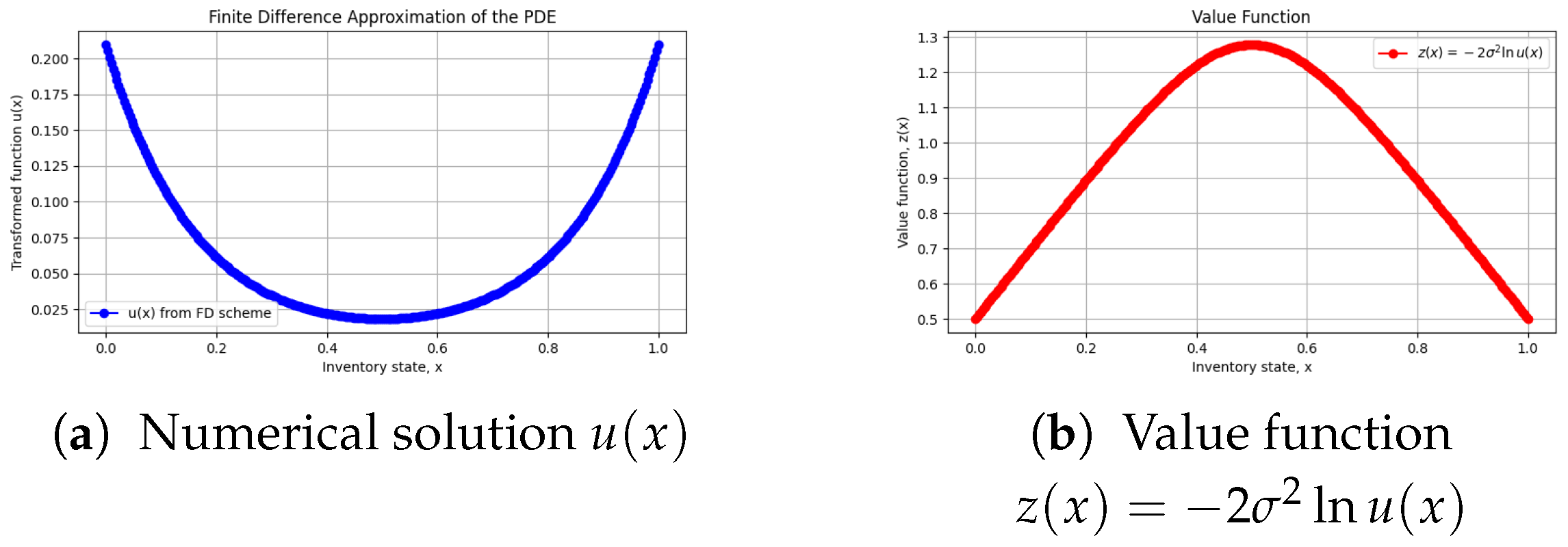
5.1.3. Numerical Results

Figure 1(left) shows $u\left(x\right)$ from the finite-difference solve, matching the boundary values exactly and exhibiting smoothness consistent with theory. Figure 1(right) shows the corresponding $z\left(x\right)$, which is concave as predicted by Theorems 1 and 2.

Figure 2(left) plots the optimal control $p^{\ast }\left(x\right)$ obtained via numerical differentiation of z. Figure 2(right) shows a sample simulated inventory trajectory under $p^{\ast }$, remaining within the safe-operating interval until the stochastic exit time. These results confirm that the curvature and stability properties of z translate into smooth, well-behaved control actions.

5.1.4. Discussion

The concavity of $z\left(x\right)$ is evident in Figure 1b and matches our analytical findings. This property ensures that $p^{\ast }$ varies smoothly, avoiding excessive corrections and supporting robust performance under stochastic perturbations. From a managerial perspective, this means that production adjustments become less aggressive as the system approaches the low-cost region, while stronger but stable corrections are applied near the boundary. Together, these figures highlight the consistent interplay between analytical structure and computational outcomes, demonstrating that the finite-difference approach effectively implements the optimal control policy in a realistic production-planning scenario.

5.2. Example 2: 2D PDE on an Elliptical Domain

We next extend the finite-difference framework to a two-dimensional elliptical domain, as implemented in Appendix A (Example 2). The admissible region $\omega$ now models the safe operating envelope for two coupled production parameters that must be controlled simultaneously.

5.2.1. Application Context

In semiconductor fabrication, process safety depends on maintaining both chemical concentration and machine utilization within prescribed bounds.

Due to joint operational and quality constraints, the feasible set is elliptical rather than rectangular. For illustration, we take a circle with semi-axes $a=1$, $b=1$ to facilitate comparison with the exact radial solution in [22], but the method accommodates general ellipses. The volatility $\sigma =0.3$ models intrinsic process noise, and the terminal cost $Z_0=0.2$ represents the economic impact of a forced shutdown.

In this setting, the computed value function $z\left(y\right)$ quantifies the minimal expected cost (or risk) associated with deviations from the optimal operating point.

The derived control field

$$p^{\ast }\left(y\right)=\left(p_1^{\ast }\left(y\right),p_2^{\ast }\left(y\right)\right)$$

prescribes real-time adjustments to drive the system toward the center of $\omega$ while respecting the domain’s geometric constraints.

The economic meaning of these parameters is as follows (

Table 2. Interpretation of variables in the semiconductor case.

Symbol	Interpretation
$y_1\left(t\right)$	Normalized chemical concentration (safe range $\approx 0.8$–$1.2$).
$y_2\left(t\right)$	Normalized equipment utilization rate (safe range $\approx 70$–$90\%$).
$\omega$	Elliptical safe-operating region capturing joint constraints.
$\sigma$	Process noise intensity (variability in both $y_1,y_2$).
$Z_0$	Shutdown/reconfiguration penalty (economic cost of exit).
$x_0$	Reference operating point (nominal safe target, here $(0,0)$).
$b\left(y\right)$	Holding cost $y_1^2+y_2^2$, penalizing deviations from $x_0$.

):

5.2.2. Algorithmic Outline

• Input: ellipse semi-axes $(a,b)$, volatility $\sigma$, terminal cost $Z_0$, grid spacing h, tolerance tol, maximum iterations max_iter.
• Output: meshgrid $(X,Y)$, solution $u\left(y\right)$, value function $z\left(y\right)$, controls $(p_1^{\ast },p_2^{\ast })$.
• Discretize the bounding rectangle and mark interior points satisfying

  $${(x/a)}^2+{(y/b)}^2<1.$$
• Impose Dirichlet boundary condition

  $$u\equiv e^{-Z_0/\left(2{\sigma }^2\right)}\mathrm{on}\partial \omega .$$
• Initialize u in the interior; define

  $$b\left(y\right)=y_1^2+y_2^2.$$
• Iterate Gauss-Seidel updates on interior points until convergence.
• Compute

  $$z\left(y\right)=-2{\sigma }^{2}lnu\left(y\right).$$
• Approximate ${\partial }_{y_1}z$ and ${\partial }_{y_2}z$ by centered differences.
• Set

  $$p_i^{\ast }\left(y\right)=-\frac{1}{2}{\partial }_{y_i}z\left(y\right),i=1,2.$$

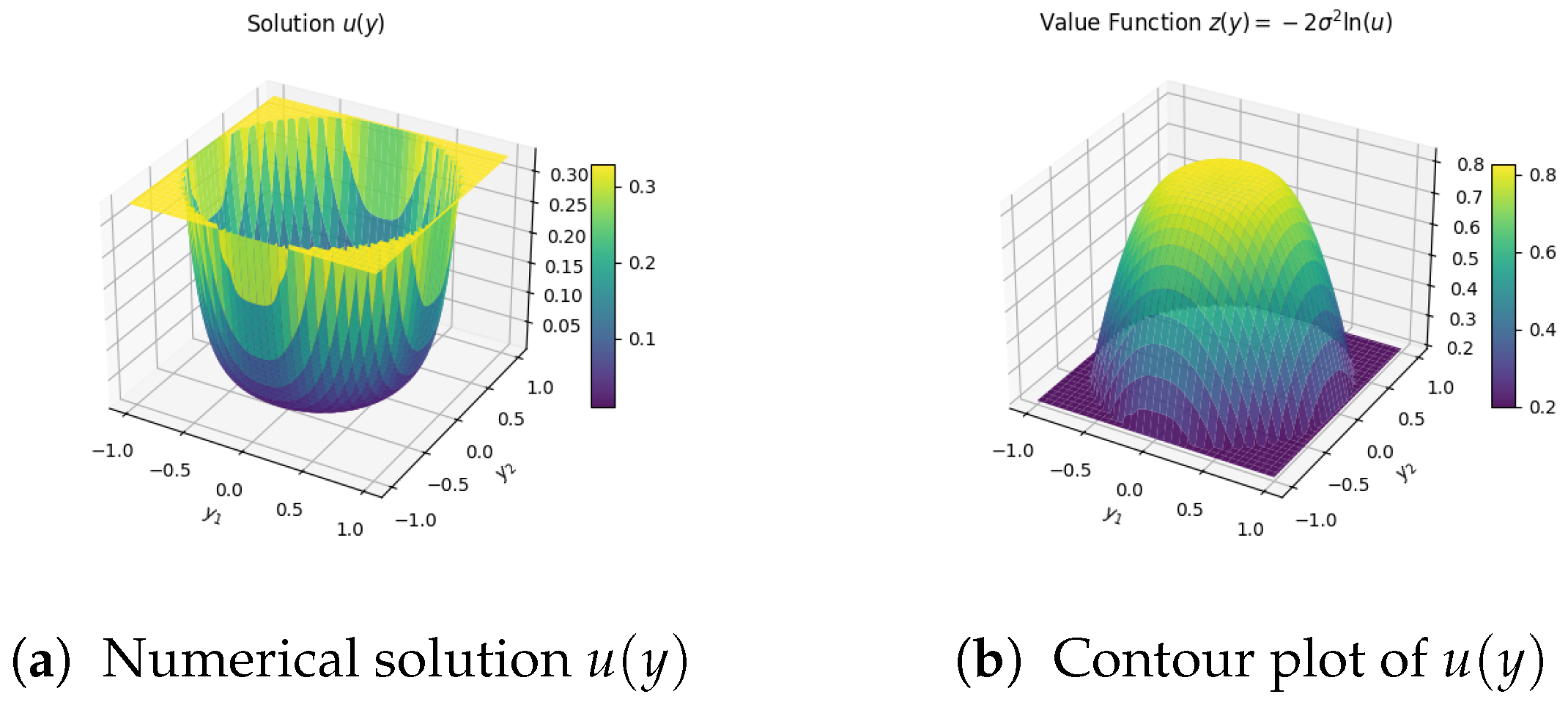
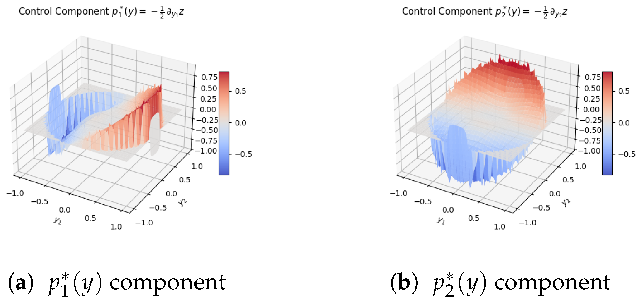
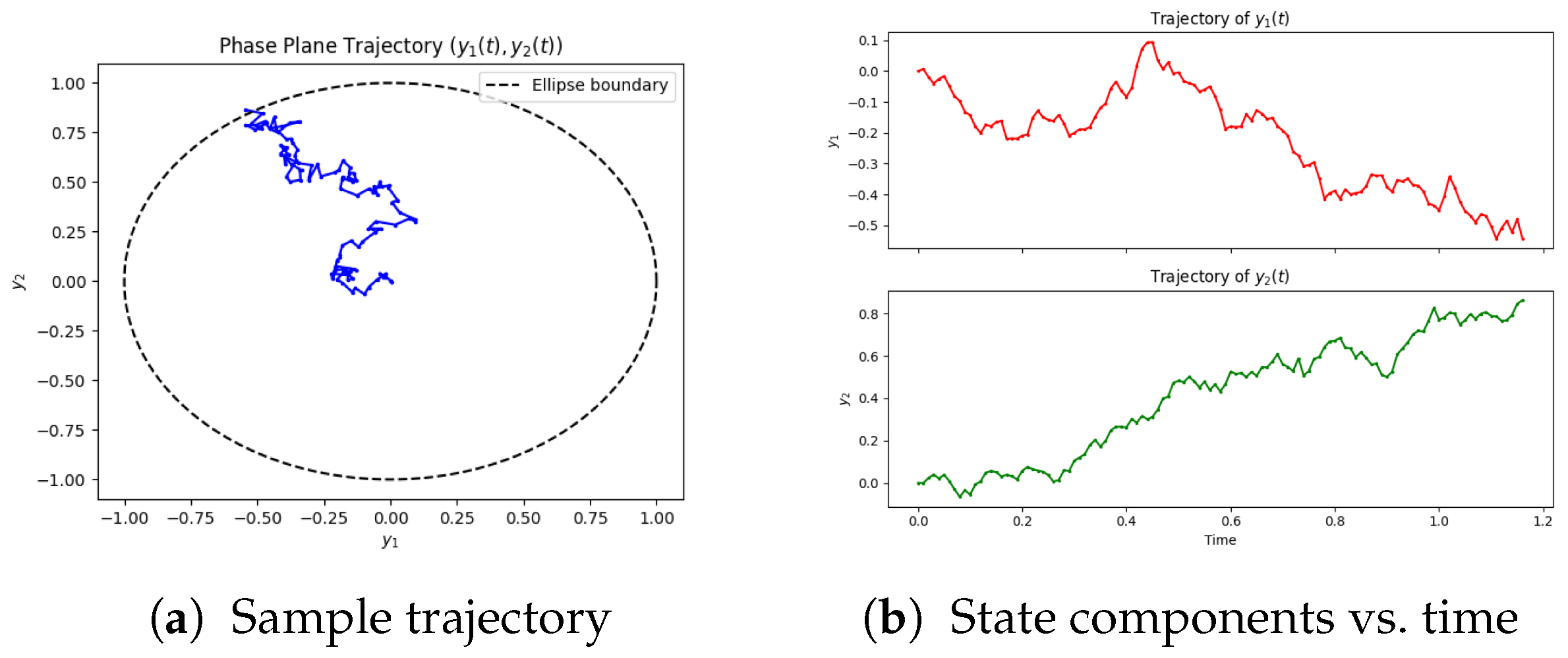
5.2.3. Numerical Results

Figure 3 shows the finite-difference solution $u\left(y\right)$ for the elliptical domain. The color map reveals how the geometry influences u, and when $b\left(y\right)$ is radially symmetric, the solution is correspondingly symmetric, in agreement with [19].

The optimal feedback controls $p^{\ast }\left(y\right)$, computed from $\nabla z\left(y\right)$, are shown in Figure 4 as vector fields. They point toward the domain center, with increased magnitude near the boundary, reflecting the stronger corrective actions required close to capacity limits.

Finally, Figure 5 shows a simulated inventory trajectory under $p^{\ast }$ using the Euler–Maruyama method. The path remains within $\omega$ until the stopping time; as $\parallel y\left(t\right)-x_0\parallel$ approaches $\mathrm{dist}(x_0,\partial \omega )$, $p^{\ast }$ increases in magnitude to avert exit.

5.2.4. Discussion

These simulations confirm the smoothness, concavity, and optimality properties predicted in Section 3 and Section 4. The finite-difference method captures the influence of domain geometry on the value function and control laws, thus validating the practical applicability of our stochastic production planning framework to multi-parameter systems. From a managerial perspective, the results show the following:

• Joint safety constraints (ellipse) lead to different corrective patterns than independent per-variable bounds.
• Concavity of z ensures that feedback controls avoid oscillations, providing robustness against noise.
• The reference point $x_0$ acts as the nominal safe operating point; sensitivity analysis indicates that shifting $x_0$ changes the stopping time $\tau$ and total cost $J\left(p\right)$, highlighting its importance in practice. Mathematically, the stopping condition corresponds to the inventory level y exiting the admissible domain $\omega$. In our implementation, this condition is imposed primarily to ensure numerical tractability within the Python-based finite-difference scheme.

6. Conclusions and Future Directions

We presented a stochastic production planning framework that explicitly incorporates geometric capacity constraints via a smooth convex operating domain. By transforming the Hamilton–Jacobi–Bellman (HJB) equation, we established the existence, uniqueness, strict positivity, and convexity of the transformed solution u, as well as the concavity of the value function $z=-2{\sigma }^{2}logu$. We derived boundary gradient asymptotics that quantify the intensity of optimal corrective actions near capacity limits and verified the optimality through a martingale argument, yielding a feedback control $p^{\ast }\left(y\right)=-\frac{1}{2}\nabla z\left(y\right)$. Finite-difference implementations in one and two dimensions demonstrated how the domain geometry shapes both the value function and the policy and showed how the feedback stabilizes inventory trajectories under stochastic fluctuations.

6.1. Managerial Interpretation

The concavity of z implies diminishing marginal cost reductions near low-cost regions, making $p^{\ast }$ smoother and more robust to noise. The boundary gradient characterization explains why control intensity rises near capacity limits: sharper, yet stable, adjustments prevent risky excursions. In practice, these properties translate into implementable rules that proactively steer operations away from unsafe zones and justify temporary halts when excursions are likely. Compared to classical inventory models with separable constraints, our framework highlights how joint geometric constraints fundamentally alter both the shape of the value function and the structure of optimal policies.

6.2. Role of the Stopping Rule

The stopping rule (1) is central to both modeling realism and analytical tractability:

• Risk management. Exiting the safe-operating set triggers a halt, preventing overloads, quality failures, or regulatory breaches.
• Well-posedness and finite cost. With production halted at $\tau$, the cost

  $$J\left(p\right)=\mathbb{E}\left[{\int }_0^{\tau }\left({\parallel p\left(t\right)\parallel }^2+b\left(y\left(t\right)\right)\right)dt\right]$$

  remains finite, enabling rigorous HJB analysis and reliable numerics.
• Geometry-aware control design. The control law accounts for joint capacity constraints encoded by $\omega$, avoiding operating regimes where the model or process becomes unreliable.
• Practical alignment. The exit policy formalizes standard operating procedures: intervene early, halt safely when necessary, and resume after corrective measures.

6.3. Limitations and Extensions

The current analysis assumes a smooth convex domain, isotropic noise, and quadratic effort costs. Demand dynamics, backlog/shortage penalties, and setup costs are not explicitly modeled, and the exit policy may be conservative relative to reflecting or soft-constraint alternatives. Several extensions can enhance both the realism and scope:

• Richer economics. Incorporate demand and backlog dynamics, service levels, and capacity adjustment or setup costs; consider risk-sensitive criteria (e.g., CVaR).
• General domains and constraints. Address nonconvex or time-varying feasible sets, soft constraints, reflecting boundaries, or state-dependent volatility and coupling.
• Partial information and learning. Study noisy state observations, parameter uncertainty, and data-driven estimation of $b\left(y\right)$; integrate robust or adaptive control.
• High-dimensional numerics. Develop scalable solvers (FEM, multigrid, domain decomposition, policy iteration), and explore machine-learning PDE solvers (e.g., deep Galerkin methods, PINNs) for complex geometries.
• Model predictive control (MPC). Combine the HJB-based policy with receding-horizon optimization for disturbance rejection and constraint handling on plant-floor timescales.

6.4. Closing Statement

Overall, the proposed framework connects rigorous stochastic control with actionable production policies that respect joint capacity limits. The analytical guarantees support reliable computation and interpretation, while the numerical studies illustrate how geometry, uncertainty, and cost structure jointly determine optimal operational decisions. By bridging mathematical rigor with managerial insight, this work lays the foundation for future research on geometry-aware, risk-sensitive, and computationally scalable production planning.

References

- Zhang, X.; Li, Y.; Guo, J. The Role of Longevity-Indexed Bond in Risk Management of Aggregated Defined Benefit Pension Scheme. Risks 2024, 12, 49. [Google Scholar] [CrossRef]
- Covei, D.-P. Image Restoration via Integration of Optimal Control Techniques and the Hamilton–Jacobi–Bellman Equation. Mathematics 2025, 13, 3137. [Google Scholar] [CrossRef]
- Tang, C.; Li, X.; Wang, Q. Mean-Field Stochastic Linear Quadratic Optimal Control for Jump-Diffusion Systems with Hybrid Disturbances. Symmetry 2024, 16, 642. [Google Scholar] [CrossRef]
- Gharbi, A.; Kenné, J.-P.; Takengny, A.L.K.; Assid, M. Joint Emission-Dependent Optimal Production and Preventive Maintenance Policies of a Deteriorating Manufacturing System. Sustainability 2024, 16, 6146. [Google Scholar] [CrossRef]
- Kenné, J.-P.; Gharbi, A.; Takengny, A.L.K.; Assid, M. Optimal Control Policy of Unreliable Production Systems Generating Greenhouse Gas Emission. Sustainability 2024, 16, 5760. [Google Scholar] [CrossRef]
- Kováts, P.; Skapinyecz, R. A Combined Capacity Planning and Simulation Approach for the Optimization of AGV Systems in Complex Production Logistics Environments. Logistics 2024, 8, 121. [Google Scholar] [CrossRef]
- Cadenillas, A.; Lakner, P.; Pinedo, M. Optimal control of a mean-reverting inventory. Oper. Res. 2010, 58, 1697–1710. [Google Scholar] [CrossRef]
- Cadenillas, A.; Lakner, P.; Pinedo, M. Optimal production management when demand depends on the business cycle. Oper. Res. 2013, 61, 1046–1062. [Google Scholar] [CrossRef]
- Gharbi, A.; Kenne, J.P. Optimal production control problem in stochastic multiple-product multiple-machine manufacturing systems. IIE Trans. 2003, 35, 941–952. [Google Scholar] [CrossRef]
- Sethi, S.P.; Thompson, G.L. Applied Optimal Control: Applications to Management Science; Nijhoff: Boston, MA, USA, 1981. [Google Scholar]
- Thompson, G.L.; Sethi, S.P.; Teng, J. Strong planning and forecast horizons for a model with simultaneous price and production decisions. Eur. J. Oper. Res. 1984, 16, 378–388. [Google Scholar] [CrossRef]
- Alvarez, O. A quasilinear elliptic equation in . Proc. R. Soc. Edinb. Sect. A 1996, 126, 911–921. [Google Scholar] [CrossRef]
- Lasry, J.M.; Lions, P.L. Nonlinear elliptic equations with singular boundary conditions and stochastic control with state constraints. Math. Ann. 1989, 283, 583–630. [Google Scholar] [CrossRef]
- Gilbarg, D.; Trudinger, N.S. Elliptic Partial Differential Equations of Second Order; Springer: Berlin/Heidelberg, Germany; New York, NY, USA, 1977. [Google Scholar]
- Amann, H. Fixed Point Equations and Nonlinear Eigenvalue Problems in Ordered Banach Spaces. SIAM Rev. 1976, 18, 620–709. [Google Scholar] [CrossRef]
- Lieberman, G.M. Asymptotic Behavior and Uniqueness of Blow-up Solutions of Quasilinear Elliptic Equations. J. Anal. Math. 2011, 115, 213–249. [Google Scholar] [CrossRef]
- Lieberman, G.M. Gradient estimates for singular fully nonlinear elliptic equations. Nonlinear Anal. 2015, 119, 382–397. [Google Scholar] [CrossRef]
- Lieberman, G.M. Gradient estimates for elliptic oblique derivative problems via the maximum principle. Adv. Differ. Equ. 2020, 25, 709–754. [Google Scholar] [CrossRef]
- Covei, D.-P. Stochastic Production Planning: Optimal Control and Analytical Insights. arXiv 2025, arXiv:2505.12341. [Google Scholar] [CrossRef]
- Brascamp, H.J.; Lieb, E.H. On extensions of the Brunn–Minkowski and Prékopa–Leindler theorems, including inequalities for log concave functions, and with an application to the diffusion equation. J. Funct. Anal. 1976, 22, 366–389. [Google Scholar] [CrossRef]
- Korevaar, N. Convex solutions of nonlinear elliptic and parabolic boundary value problems. Indiana Univ. Math. J. 1987, 36, 687–704. [Google Scholar]
- Canepa, E.C.; Covei, D.-P.; Pirvu, T.A. A stochastic production planning problem. Fixed Point Theory 2022, 23, 179–198. [Google Scholar] [CrossRef]
- Kloeden, P.E.; Platen, E. Numerical Solutions of Stochastic Differential Equations; Applications of Mathematics; Springer: New York, NY, USA, 1992; Volume 23. [Google Scholar]
- Talay, D.; Tubaro, L. Expansion of the Global Error for Numerical Schemes Solving Stochastic Differential Equations. Stoch. Anal. Appl. 1990, 8, 483–509. [Google Scholar] [CrossRef]
- Bayer, C. Discretization of SDEs: Euler Methods and Beyond. 2006. Available online: https://wias-berlin.de/people/bayerc/files/euler_talk_handout.pdf (accessed on 19 August 2025).
- Bayram, M.; Partal, T.; Buyukoz, G.O. Numerical methods for simulation of stochastic differential equations. Adv. Contin. Discret. Model. 2018, 2018, 17. [Google Scholar] [CrossRef]
- Holmes-Cerfon, M. Applied Stochastic Analysis; American Mathematical Society, Courant Institute of Mathematical Sciences at New York University: New York, NY, USA, 2024; Volume 33. [Google Scholar]