Article

Non-Uniformly Multidimensional Moran Random Walk with Resets

by
Mohamed Abdelkader
Department of Statistics and Operations Research, College of Science, King Saud University, P.O. Box 2455, Riyadh 11451, Saudi Arabia
Axioms 2025, 14(10), 756; https://doi.org/10.3390/axioms14100756
Submission received: 26 August 2025 / Revised: 29 September 2025 / Accepted: 3 October 2025 / Published: 7 October 2025
(This article belongs to the Section Mathematical Analysis)

Abstract

In this paper, we investigate the non-uniform m-dimensional Moran walk ( Z n ( 1 ) , , Z n ( m ) ) , where each component process ( Z n ( j ) ) 1 j m , either increases by one unit or resets to zero at each step. Using probability generating functions, we analyze key statistical properties of the walk, with particular emphasis on the mean and variance of its final altitude. We further establish closed-form expressions for the limiting distribution of the process, as well as for the mean and variance of each component. These results extend classical findings on one- and two-dimensional Moran models to the general m-dimensional setting, thereby providing new insights into the asymptotic behavior of multi-component random walks with resets.
MSC:
60C05; 60F99; 60E05; 60G40

1. Introduction

Understanding the behavior of high-dimensional stochastic systems remains a central challenge in probability theory and its applications. In particular, multi-component discrete random walks, such as the high-dimensional Moran walk, provide a versatile framework for modeling sequences of random steps in multiple dimensions. These models are especially relevant for describing complex phenomena in population genetics [1,2,3], wave propagation [4], and other areas of science. Despite their widespread use, explicit characterizations of their statistical properties, such as limiting distributions, means, and variances, remain largely unexplored in higher dimensions [5].
Several studies have addressed aspects of this problem. Using probability generating functions, the kernel method, and singularity analysis, researchers have investigated the asymptotic behavior of higher-dimensional discrete random walks [6,7,8]. In the two-dimensional Moran model, Althagafi and Abdelkader [9] established that the age of each component converges asymptotically to a shifted geometric distribution, while Aguech and Abdelkader [10] analyzed the final altitude and the number of resets. Similarly, Itoh and Mahmoud [3] studied age structures in population genetics models, deriving shifted geometric limits for individual lifetimes, and Itoh, Mahmoud, and Takahashi [4] proved the existence of stationary distributions as convolutions of geometric random variables and established normality results for wavelength distributions in stochastic soliton models. Aguech, Althagafi, and Banderier [5] analyzed one- and multi-dimensional Moran walks and showed that their heights asymptotically follow a discrete Gumbel distribution. Other related contributions include [11,12].
The goal of this work is to extend the analysis of Moran-type random walks to a general non-uniform m-dimensional setting. Specifically, we investigate the process ( Z n ( 1 ) , , Z n ( m ) ) , where each component Z n ( j ) , 1 j m , either increments by one or resets to zero at each step. Using probability generating functions, we derive explicit expressions for key statistical properties, including the mean and variance of the final altitude, as well as the limiting distributions and moments of each component. Compared to the classical studies of one- and two-dimensional Moran models [9,10,13], our results generalize the theoretical framework to arbitrary dimensions, providing new insights into the asymptotic behavior of multi-component random walks with resets. In particular, while Mahmoud [3] focused on the distribution of gamete ages and related combinatorial structures in low-dimensional Moran models, our study extends these findings to higher dimensions, allowing for the analysis of interactions among multiple components and offering a broader probabilistic perspective on complex stochastic systems.
Our model (6) is very important and applicable in many fields. The model (6) can also be interpreted in the context of gamete evolution in a finite population, following the framework of Mahmoud and Ito [3]. Here, each component Z n ( j ) represents the “age” of gamete type j at generation n, defined as the number of generations since a mutation or recombination event created a new representative of this type. With probability p ^ , a global event such as selection or genetic bottleneck replaces all gametes, resetting the age of every type to zero. With probability p j , a gamete of type j is reproduced or survives preferentially, incrementing its age while all other types are reset, reflecting competition between gamete lineages. With probability p ¯ , all gametes survive and reproduce simultaneously, resulting in a uniform increment of ages across types. Within this interpretation, the closed-form results for the limiting distributions, means, and variances of Z n ( j ) and Z ˜ n allow quantification of key evolutionary statistics, such as the expected age of the oldest gamete type, the distribution of inter-generation lineage durations, and the impact of selection and bottleneck events on genetic diversity.
In this work, we provide closed-form expressions for the mean and variance of the final altitude using probability generating functions. We also study the limiting distributions, means, and variances of the individual random walks, thereby extending existing results to higher-dimensional settings.
The paper is organized as follows. Section 2 introduces the higher-dimensional Moran random walk. Section 3 presents our main results on the statistical properties of the final altitude. In Section 4, we give some numerical examples. Section 5 studies recursive relations among multivariate polynomials g n ( z ) to g n 1 ( z ˜ j ) , and g n 1 ( z ) , where z = ( z 1 , , z m ) R m and z ˜ j = ( 1 , , 1 , z j , 1 , , 1 ) R m at two consecutive times n 1 and n. Section 6 proves that each random walk Z n ( j ) , where 1 j m converges asymptotically to a shifted geometric distribution with parameter 1 b j , where b j = p j + p ¯ , and provides explicit formulas for their means and variances. Section 7 concludes the paper and outlines directions for future work. Appendix A and Appendix B provide detailed proofs of the results in Section 3, Section 4, Section 5 and Section 6.

2. Presentation of the Model

We consider discrete random walks in higher dimensions with non-uniform probabilities. Precisely, we consider random walks Z n = ( Z n ( 1 ) , , Z n ( m ) ) with m components ( m 1 and n 0 ), defined as follows: at time 0, the walk Z n starts from the origin Z 0 = 0 * = 0 , , 0 , m-tuple of zeros. For each unit of time, Z n moves by one positive unit for the jth-element with probability p j ; or resets to 0 * with probability p ^ ; or shifts one unit in the m-directions with probability p ¯ under the following condition p ^ + p ¯ + j = 1 m p j = 1 .
Mathematically, our model is given by the following system:
Z n + 1 = ( Z n + 1 ( 1 ) , , Z n + 1 ( m ) ) = ( 0 , 0 , , 0 ) , with probability p ^ , ( 0 , , 0 , Z n ( j ) + 1 , 0 , , 0 ) , with probability p j , ( Z n ( 1 ) + 1 , , Z n ( m ) + 1 ) , with probability p ¯ ,
satisfying the following condition
p ¯ + p ^ + i = 1 m p j = 1 ,
where p j , 1 j m , p ¯ and p ^ are probabilities.
Definition 1.
Let ( Z n ) n 0 be a Moran random walk taking values in N m , where
Z n = Z n ( 1 ) , Z n ( 2 ) , , Z n ( m ) ,
denotes the vector of its m components at time n.
1. 
We define the walk ( Z ˜ n ) n N , called final altitude (maximum) of the walk ( Z n ) n N , at time n by
Z ˜ n = max ( Z n ) : = max { Z n ( 1 ) , , Z n ( m ) } .
2. 
Furthermore, we introduce the process ( H n ) n 0 , called height statistics, as the maximum of ( Z ˜ n ) , that is, at time n
H n = max Z ˜ 0 , Z ˜ 1 , , Z ˜ n .
Example 1.
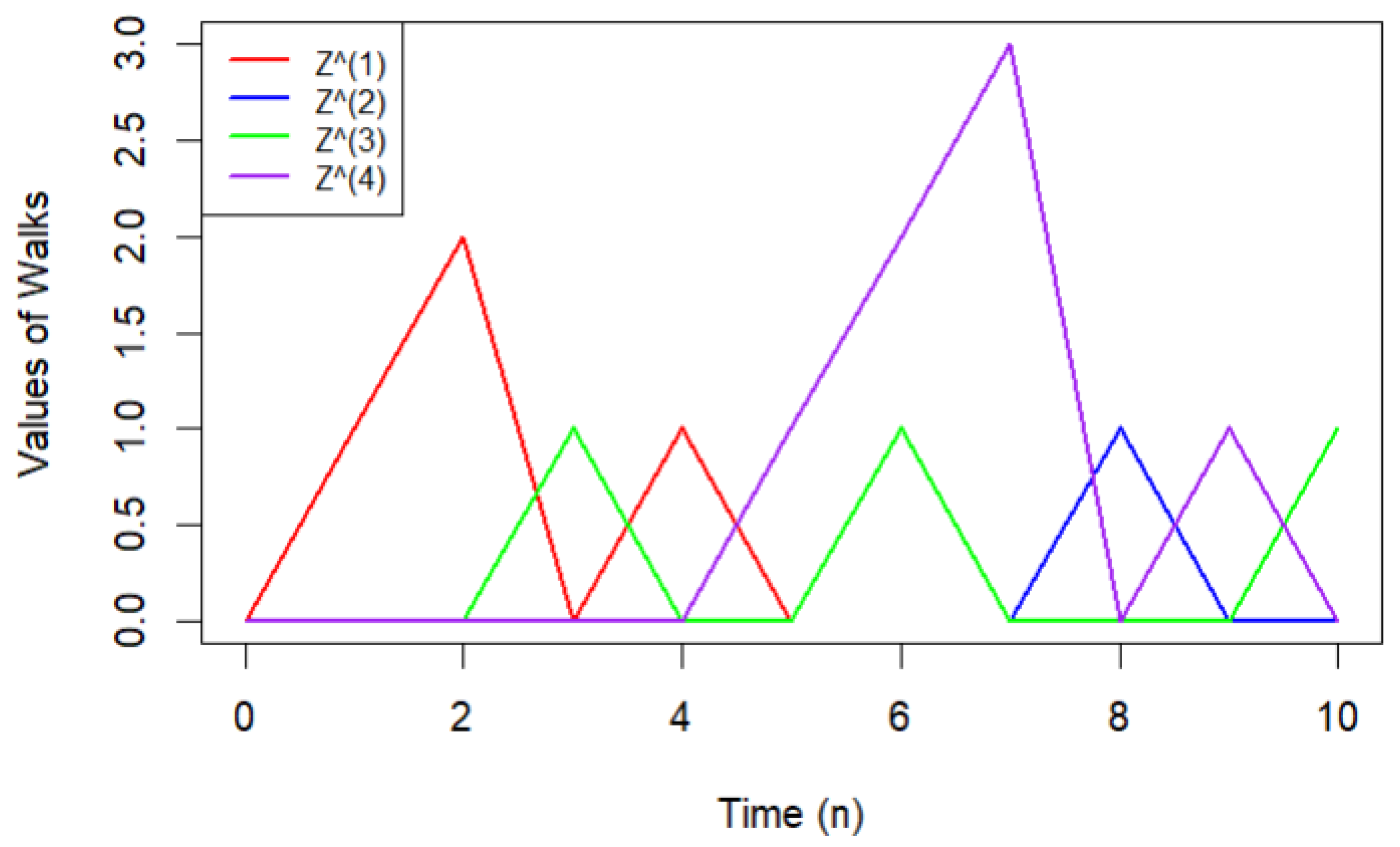
In this example, we consider a 4-dimensional random Moran ( m = 4 ) walk with length n = 10 and with initial probabilities p ¯ = p ^ = 0.1 , and p 1 = p 2 = p 3 = p 4 = 0.2 .
Figure 1 shows that the evolution of Z 10 ( 1 ) , Z 10 ( 2 ) , Z 10 ( 3 ) , Z 10 ( 4 ) , respectively, is given by:
0 1 2 0 1 0 1 0 0 0 0 , 0 0 0 0 0 0 1 0 1 0 0 , 0 0 0 1 0 0 1 0 0 0 1 , 0 0 0 0 0 1 2 3 0 1 0 .
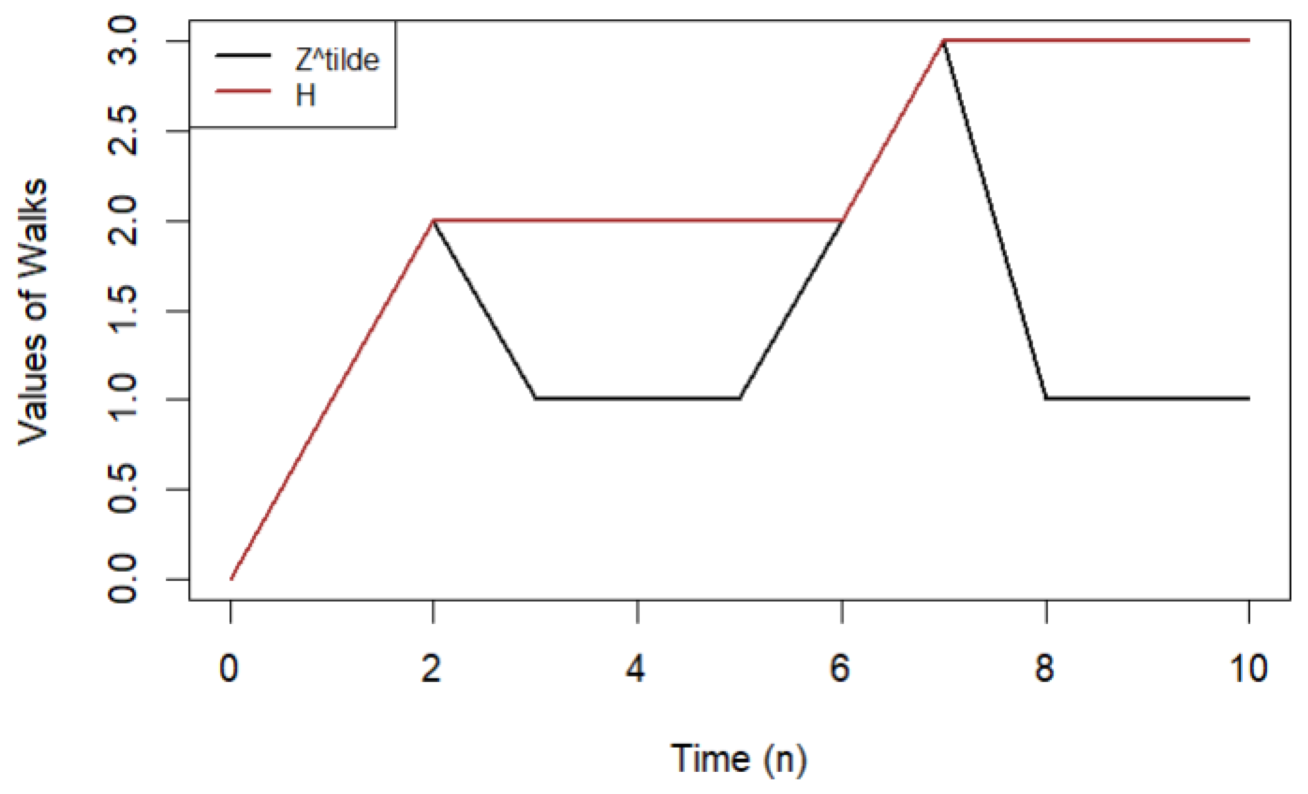
Figure 2 shows that the evolution of Z ˜ 10 , H 10 , respectively, is given by:
0 1 2 1 1 1 2 3 1 1 1 , 0 1 2 2 2 2 2 3 3 3 3 .
At each unit of time k, the final altitude takes the maximum value between the four walks Z n ( 1 ) , Z n ( 2 ) , Z n ( 3 ) and Z n ( 4 ) . In our example, if k = 6 , then we have Z ˜ 6 = max ( Z 6 ( 1 ) , Z 6 ( 2 ) , Z 6 ( 3 ) , Z 6 ( 4 ) ) = max ( 1 , 1 , 1 , 2 ) = 2 . Furthermore, at time k, the height statistics H k takes the maximum value between Z ˜ 0 , , Z ˜ k . In our example H 6 = max ( 0 , 1 , 2 , 1 , 1 , 1 , 2 ) = 2 (see Figure 2).
In the next section of this work, the mean and variance of the random walks Z n ( j ) , j = 1 , 2 , , m , are represented by μ j and σ j 2 . We present the two following important relations concerning the link between the mean and the variance of a discrete random variable Y and its probability generating function G Y ( y ) when the first and the second derivatives of G Y ( y ) exist at y = 1 :
μ Y = G Y ( y ) y | y = 1 a n d σ Y 2 = 2 G Y ( y ) 2 y | y = 1 + E Y E Y 2 .
Figure 1. Evolution of the walks Z 10 ( 1 ) , Z 10 ( 2 ) , Z 10 ( 3 ) , Z 10 ( 4 ) with initial probabilities p ¯ = p ^ = 0.1 and p 1 = p 2 = p 3 = p 4 = 0.2 .
Axioms 14 00756 g001
Figure 2. Evolution of the final altitude Z ˜ 10 and the height statistics H 10 with initial probabilities p ¯ = p ^ = 0.1 and p 1 = p 2 = p 3 = p 4 = 0.2 .
Axioms 14 00756 g002

3. Main Result

Our objective in this section is to establish the explicit expressions for the mean and the variance of the random walk Z ˜ n = max ( Z n ( 1 ) , , Z n ( m ) ) . For this, we find the closed expression of the probability generating function of Z ˜ n , denoted by φ n ( t ) , and defined by: t R , j { 1 , , m }
φ n ( t ) = φ Z ˜ n ( t ) = h = 0 n t h P ( Z n = h ) = h = 0 n t h P max ( Z n ( 1 ) , , Z n ( m ) ) = h .
In the next theorem, we find the explicit expression of the probability generating function φ n ( t ) of the random walk Z ˜ n . It is a very important tool and used to find some statistical properties such as the mean and the variance of the final altitude Z ˜ n .
Theorem 1.
The probability generating function, φ n ( t ) , of the final altitude Z ˜ n , is given by: t R and n 0
φ n ( t ) = ( p ¯ t ) n + p ^ 1 p ¯ t 1 ( p ¯ t ) n + j = 1 m b j b j n p ¯ n t n 1 t 1 b j t + p j t 1 b j 1 b j t 1 p ¯ t n 1 p ¯ t .
such that b j = p j + p ¯ , | b j t | < 1 and | p ¯ t | < 1 .
The detailed proof of this theorem is presented in Appendix B.
Comment 1.
We discuss some comments from Theorem 1
1. 
Theorem 1 provides an explicit expression for the probability generating function (PGF)  φ n ( t )  of the final altitude  ( Z ˜ n ) n N  of the m-dimensional Moran walk. The PGF encodes all probabilistic information about  ( Z ˜ n ) n N , allowing computation of moments (mean, variance) and, in principle, the full distribution.
2. 
The Formula (4) can be interpreted as the sum of three contributions:
  • ( p ¯ t ) n  corresponds to the scenario where all components increment together at each step, i.e., no resets occur.
  • p ^ 1 p ¯ t 1 ( p ¯ t ) n  accounts for global resets with probability p ^  , producing a geometric-like contribution across all components.
  • The summation term  j = 1 m [ ]  captures single-component increments and partial resets, reflecting the combined effects of individual growth probabilities  p j  and the collective increment  p ¯ .
3. 
This PGF generalizes classical results for one-dimensional, two-dimensional, (Theorem 1 in [9]), three-dimensional Moran walks (Theorem 1 in [13]) to arbitrary m-dimensional systems.
4. 
It captures both uniform and non-uniform increment probabilities, making it applicable to multi-component processes such as multi-strain epidemic models or gamete age dynamics.
In the next corollary, we deduce the probability generating function φ n ( t ) for one, two, and three dimensions from Equation (4).
Corollary 1.
Thus, we have
1. 
In one dimension m = 1 , the model (6) is equivalent to the following model
Z n + 1 = 0 , with probability p ^ , 1 , with probability p ¯ ,
with the probability generating function given by
φ n ( t ) = ( p ¯ t ) n + p ^ 1 p ¯ t 1 ( p ¯ t ) n , b 1 = p ¯ , w h e r e p ^ + p ¯ = 1 .
2. 
In two dimensions m = 2 , the model (6) is equivalent to the following model
Z n + 1 = ( Z n + 1 ( 1 ) , Z n + 1 ( 2 ) ) = ( 0 , 0 ) , with probability p ^ , ( 1 , 0 ) , with probability p 1 , ( 0 , 1 ) , with probability p 2 , ( 1 , 1 ) , with probability p ¯ ,
with the probability generating function given by:
φ n ( t ) = ( p ¯ t ) n + p ^ 1 p ¯ t 1 ( p ¯ t ) n + j = 1 2 b j b j n p ¯ n t n 1 t 1 b j t + p j t 1 b j 1 b j t 1 p ¯ t n 1 p ¯ t .
3. 
In three dimensions m = 3 , the model (6) is equivalent to the following model
Z n + 1 = ( Z n + 1 ( 1 ) , Z n + 1 ( 2 ) ) = ( 0 , 0 ) , with probability p ^ , ( 1 , 0 ) , with probability p 1 , ( 0 , 1 ) , with probability p 2 , ( 1 , 1 ) , with probability p ¯ ,
with the probability generating function given by:
φ n ( t ) = ( p ¯ t ) n + p ^ 1 p ¯ t 1 ( p ¯ t ) n + j = 1 3 b j b j n p ¯ n t n 1 t 1 b j t + p j t 1 b j 1 b j t 1 p ¯ t n 1 p ¯ t .
In the next theorem, we derive the mean and variance of the walk Z ˜ n from φ n ( t ) .
Theorem 2.
The mean and variance of the final altitude Z n are given by:
E Z ˜ n = ( m 1 ) p ¯ 1 p ¯ n 1 p ¯ + j = 1 m b j 1 b j n 1 b j , V a r ( Z ˜ n ) = 2 n m 1 p ¯ n + 1 1 p ¯ 2 m 1 p ¯ 2 p ¯ n + 2 1 p ¯ 2 + 2 j = 1 m b j b j n b j n 1 b j + b j 2 b j b j n 1 b j 2
+ j = 1 m b j b j n + 1 1 b j ( m 1 ) p ¯ p ¯ n + 1 1 p ¯ j = 1 m b j b j n + 1 1 b j ( m 1 ) p ¯ p ¯ n + 1 1 p ¯ 2 ,
such that b j = p j + p ¯ , 1 j m .
The proof of this theorem is provided in Appendix B.
Comment 2.
Theorem 2 provides explicit formulas for the mean and variance of the final altitude  Z ˜ n  in the m-dimensional Moran walk with resets. These expressions are derived directly from the probability generating function  φ n ( t )  presented in Theorem 1.
1. 
Mean  E ( Z ˜ n ) : The first term,  ( m 1 ) p ¯ 1 p ¯ n 1 p ¯ , represents the contribution of the global reset events, which effectively reduce the growth of the maximum altitude across the m components. The summation term  j = 1 m b j ( 1 b j n ) 1 b j  captures the cumulative effect of individual component increments and combined increments, weighted by  b j = p j + p ¯ .
2. 
Variance  V a r ( Z ˜ n ) : The variance formula is more complex, reflecting the interplay between global resets and individual increments. The first two terms account for correlations introduced by global resets, while the summation over j captures the variance contribution of each component’s individual dynamics. The final two terms adjust for the square of the mean to ensure the correct computation of variance.
3. 
These formulas explicitly show how both the number of components m and the probabilities  p ¯ , p j  influence the expected final altitude and its variability.
4. 
These explicit results allow quantitative analysis of multi-component stochastic systems, such as the expected maximum age of gametes, times between outbreaks in multi-strain epidemic models, or other processes modeled by high-dimensional Moran walks.
Theorem 2 extends classical one- and two-dimensional Moran walk results to arbitrary m dimensions and provides practical formulas for both theoretical analysis and simulation validation.
In the next corollary, we present the mean and variance of the random walk  Z n , for one and two dimensions. It suffices to take  m = 1 and m = 2  in Equations (7) and (8).
Corollary 2.
we have
1. 
In one dimension m = 1 ,
E Z ˜ n = p ¯ p ¯ n + 1 1 p ¯ , V a r ( Z ˜ n ) = 2 p ¯ p ¯ n p ¯ n 1 p ¯ + p ¯ 2 p ¯ p ¯ n 1 p ¯ 2 + p ¯ p ¯ n + 1 1 p ¯ p ¯ p ¯ n + 1 1 p ¯ 2 ,
2. 
In two dimensions m = 2 ,
E Z ˜ n = b 1 b 1 n + 1 1 b 1 + b 2 b 1 n + 1 1 b 2 p ¯ p ¯ n + 1 1 p ¯ , V a r ( Z ˜ n ) = 2 n p ¯ n + 1 1 p ¯ 2 p ¯ 2 1 p ¯ n 1 p ¯ 2 + 2 j = 1 2 b j b j n b j n 1 b j + b j 2 b j b j n 1 b j 2 + j = 1 2 b j b j n + 1 1 b j p ¯ p ¯ n + 1 1 p ¯ j = 1 2 b j b j n + 1 1 b j p ¯ p ¯ n + 1 1 p ¯ 2 .

4. Numerical Examples

To illustrate the model’s behavior and validate the theoretical results, we conducted a series of numerical simulations. Table 1 presents the evolution of the expectation E ( Z ˜ n ) and the variance V ar ( Z ˜ n ) of the final altitude Z ˜ n as a function of time n for three distinct sets of parameters ( p ^ , p 1 , p 2 , p 3 , p ¯ ) . These parameters allow us to explore different probability regimes for the particle’s jumps. We observe that, depending on the case, the values of E ( Z ˜ n ) and V ar ( Z ˜ n ) converge to stationary limits at different rates. For instance, in case 1, convergence is very rapid, whereas for case 3, the expectation and variance take longer to stabilize, indicating a longer transient dynamic. These numerical examples thus highlight the model’s sensitivity to the distribution of the jumps.
Table 1 reports the mean and variance of the final altitude Z ˜ n at different times n for three parameter settings corresponding to distinct values of p ¯ . In each case, the mean increases with n before stabilizing at a limiting value. In Case 1, the mean converges to approximately 1.857 , in Case 2, to about 3.233 , and in Case 3, to nearly 5.333 . Similarly, the variance shows a growth phase followed by stabilization, approaching about 4.678 in Case 1, 11.123 in Case 2, and 27.711 in Case 3.
These results highlight that higher values of p ¯ yield larger limiting values for both the mean and the variance. The convergence occurs relatively quickly, with stabilization observable already for moderate values of n. This demonstrates the strong influence of p ¯ on the long-term behavior of the process.
The sample path for Case 1 over the first 100 steps provides a perfect visual illustration of the rapid convergence and stabilization described by its statistics in Table 1.
We observe that the particle’s altitude undergoes a brief period of initial volatility but very quickly settles into a tight, steady-state fluctuation around a fixed mean level. This visual stabilization occurs within the first 15–20 steps, which aligns precisely with the data in Table 1:
  • The mean E ( Z ˜ n ) for Case 1 rises from 0.9 to approximately 1.856 by n = 15 and remains constant thereafter.
  • Similarly, its variance V ar ( Z ˜ n ) stabilizes around the value of 4.678 by n = 20 .
The empirical path in Figure 3 confirms this mathematical prediction. The absence of large swings after the very initial phase and the low amplitude of the fluctuations around the equilibrium level are the direct graphical manifestations of Case 1’s low and quickly stabilizing variance. This behavior indicates a stochastic system that reaches its stationary regime almost immediately, characterized by a high probability of transitions that keep the particle close to its mean altitude.

5. Recursive Equations

Let E b n and E b n , j be two sets defined as follows: for b = 0 , 1
E b n = b r j n = b r 1 , , r j 1 , r j , r j + 1 , , r m n , E b n , j = b r j n = b r 1 , , r j 1 , l j 1 , r j + 1 , , r m n .
Let p n ( l ) and g n ( z ) denote the probability associated with the model defined in (6), the sequence of multivariate polynomials g n ( z ) , respectively, defined as follows: n 0 , l = ( l 1 , , l m ) N m and z = ( z 1 , , z m ) R m , 1 * = 1 , , 1 , m-tuple of one:
p n ( l ) = P Z n = l = P Z n ( 1 ) = l 1 , Z n ( 2 ) = l 2 , , Z n ( m ) = l m , p 0 ( 0 * ) = 1 ,
g n ( z ) = g ( z 1 , , z m ) = E z 1 Z n ( 1 ) z m Z n ( m ) = E 0 n z 1 l 1 z m l m p n ( l ) , g 0 ( z ) = 1 .
Taking z = z ˜ j in Equation (10), we get the probability generating function of each random walk z ( j ) , denoted by g n ( z ˜ j ) , 1 j m :
g n ( z ˜ j ) = g n ( 1 , , 1 , z j , 1 , , 1 ) = E z j Z n ( j ) = E 0 n z j r j p n ( r ) .
Our goal in this section is to find the recursive equation between the sequence of multivariate polynomials g n ( z ) and g n 1 ( z ) , for z = ( z 1 , , z m ) R m at two consecutive times n 1 and n. For this, we find the explicit expression of the probability p n ( l ) , where l = ( l 1 , , l m ) { 0 , , n } m at the time n. Furthermore, the closed form of p n ( l ) is the key to find the relation between g n ( z ) and g n 1 ( z ) . In the next lemma, we find a recursive equation related to the two probabilities p n ( l ) and p n 1 ( l ) for two consecutive times n 1 and n when r , l { 0 , 1 , 2 , , n } m .
Lemma 1.
We have the following recursion of probabilities:
p n ( l ) = p ^ , if l = l 1 , l 2 , , l m = 0 * , p j E 0 n 1 , j p ( r 1 , , r j 1 , l j 1 , r j + 1 , , r n ) , if 1 l j n , l i = 0 , i j , p ¯ p n 1 ( l 1 ) , if 1 l j n , 1 j m .
Comment 3.
We discuss several remarks pertaining to the various cases of Equation (12)
1. 
Initial Condition: The first case  l = 0 *  provides the base probability  p ^ , which initializes the recursion and ensures that the probability distribution is properly defined at the starting state.
2. 
Single-component Increment: The second case describes the probability when exactly one component  l j  is nonzero and all other components are zero. It accounts for the contributions from all possible configurations of previous steps, captured by the sum over  E 0 n 1 , j . This reflects the combinatorial structure of the Moran process in a single dimension while conditioning on the previous states.
3. 
General Increment: The third case covers the situation where multiple components may be positive. Here, the recursion uses  p ¯ p n 1 ( l 1 ) , meaning that the probability of the current configuration depends linearly on the probability of the configuration at the previous step, with all components decreased by one. This highlights the memory structure of the process across steps.
Lemma 1 provides a recursive framework for computing the joint probabilities  p n ( l )  of the multidimensional Moran random walk. It separates contributions from the initial state, single-component increments, and general multi-component updates, which is crucial for deriving generating functions and later statistical properties such as means and variances.
Lemma 1 leads to a recursive equation related among g n ( z ) , g n 1 ( z ˜ j ) , and g n 1 ( z ) . This recursive equation is very important to find the distribution of the walk Z n ( j ) , 1 j n .
Proposition 1.
The sequence of multivariate polynomials g n ( z ) satisfies the recursive equation: z = z 1 , , z m R m ,
g n ( z ) = p ^ + j = 1 m p j z j g n 1 ( z ˜ j ) + p ¯ j = 1 m z j g n 1 ( z ) ,
where g 0 ( z ) = p 0 ( 0 * ) = 1 and z ˜ j = ( 1 , 1 , z j , 1 , , 1 ) R m .
Comment 4.
we discuss the following remarks:
1. 
Proposition 1 establishes a recursive relation for the sequence of multivariate polynomials  g n ( z ) , which plays a central role in characterizing the joint distribution of the multidimensional Moran random walk. Each polynomial  g n ( z ) is expressed in terms of the previous polynomial  g n 1 ( z ) , highlighting the step-by-step evolution of the process.
2. 
The summation term  j = 1 m p j z j g n 1 ( e z j )  captures the effect of incrementing each component individually. Here,  z j = ( 1 , , 1 , z j , 1 , , 1 )  ensures that only the j-th component is transformed while the others remain at 1, reflecting the non-uniform multidimensional dynamics.
3. 
The product term  p j = 1 m z j g n 1 ( z )  corresponds to simultaneous increments across all components, weighted by the probability p. This term accounts for correlated changes and ensures the polynomial fully captures multivariate interactions.
4. 
The base case  g 0 ( z ) = p 0 ( 0 * ) = 1  initializes the recursion, providing a foundation for constructing higher-order polynomials systematically.
this recursive representation is essential for computing the probability generating function of the multidimensional Moran random walk. It provides a compact way to study the evolution of moments, correlations, and extremal statistics, such as the final altitude or maximum across components.
Remark 1.
For completeness, the proofs of the results in this section are provided in Appendix A.

6. Distribution of the Random Walks Z n ( j )

In this part, our objective is to establish some statistical characteristics like the asymptotic distribution, the mean, and the variance of the final altitude of the random walk Z n ( j ) , at time n days, using a very important tool called the probability generating function. Firstly, we start to find the explicit expression of the probability generating function of each component denoted by g n ( z ) related to g n 1 ( z ˜ j ) and g n 1 ( z ) , where z = ( z 1 , , z m ) R m and z ˜ j = ( 1 , , 1 , z j , 1 , , 1 ) R m . Secondly, we show that the random walk Z n ( j ) converges to a shifted geometric distribution asymptotically. Finally, we find the closed form of the mean and the variance of our random walks.
In the next theorem, we establish the explicit expression of the probability generating function of Z n ( j ) . Also, we deduce that random walk Z n ( j ) converges to a geometric distribution with parameter 1 b j , 1 j m .
Theorem 3.
The probability generating functions of each random walk Z n ( j ) is given by:
g 0 ( z ) = 1 , g n ( z ˜ j ) = ( b j z j ) n + ( 1 b j ) 1 ( b j z j ) n 1 b j z j .
The limit distribution of Z n ( j ) converges, in law, to some shifted geometric (Geo) random variables:
Z n ( j ) G e o ( 1 b j ) 1 , 1 j m ,
where b j = p j + p ¯ , | b j z j | < 1 .
Comment 5.
We provide some interpretations and comments:
1. 
The theorem provides the explicit probability generating function  g n ( e z j )  for each component  Z n ( j )  of the multidimensional Moran random walk. This function encapsulates the full distributional information of the process and serves as a powerful tool to derive moments and other probabilistic characteristics.
2. 
The Formula (14) gives a closed-form expression for any step n, making computations of the mean, variance, and higher moments straightforward.
3. 
Equation (15) characterizes the long-term behavior of the process and confirms that the distribution stabilizes as  n .
4. 
The limiting distribution depends on the parameter  b j = p j + p ¯ , which reflects both the individual component probabilities and the global interaction term  p ¯ . This highlights the interplay between individual and collective dynamics in the Moran walk.
Theorem 3 not only provides exact PGFs for finite n but also identifies the asymptotic behavior of each component. This is crucial for studying extremal properties, generating functions of sums, and other derived quantities in the multidimensional setting.
Driving the probability generating function,  g n ( z ˜ j ) , of the random walk Z n ( j ) , the explicit expressions of the means and the variances of the random walks ( Z n ( j ) ) 1 j m are deduced directly.
Corollary 3.
The explicit expressions of the mean and the variance of the Moran random walks ( Z n ( j ) ) 1 j m are given by:
μ j = b j b j n + 1 1 b j a n d σ j 2 = b j ( 1 b j ) 2 1 b j n b j n + 1 + ( 1 + 2 n ) ( 1 b j ) ,
where ( b j ) 1 j n is defined in Theorem 3.
Remark 2.
For completeness, we present the proofs of the results from this section in Appendix A.

7. Conclusions and Perspectives

In this work, we have investigated the statistical properties of the non-uniform multidimensional Moran random walk ( Z n ) n N = ( Z n ( 1 ) , , Z n ( m ) ) . We established that each component process ( Z n ( j ) ) n N converges to a shifted geometric distribution with parameter b j = p j + p ¯ . Using the probability generating function, we derived closed-form expressions for the mean and variance of each component, which depend explicitly on b j and the step n. Furthermore, we analyzed the final altitude (maximum) of the walk, ( Z ˜ n ) n N , and obtained its generating function, allowing explicit computation of its mean and variance.
This analysis provides a comprehensive understanding of both the individual component dynamics and the extremal behavior of the multidimensional Moran random walk. These results not only summarize the main findings of our study but also open avenues for future research, such as extending the model to more general distributions or exploring applications in population dynamics and related stochastic processes.
Building on the results of this work, several avenues for future research can be pursued:
  • Generalization of reset mechanisms: How do the statistical properties of the multidimensional Moran walk change if resets follow more general distributions (e.g., non-geometric, state-dependent, or time-varying probabilities) rather than the uniform or fixed-probability resets considered here?
  • Interaction between components: Can we extend the model to include dependencies or interactions between components, such as coupled increments or correlated reset events, and characterize their impact on the mean, variance, and extremal behavior?
  • Continuous-time extensions: How would the results change if the model is formulated in continuous time, leading to a multidimensional Poisson or jump process analog of the Moran walk?
  • Application to population dynamics: How can the m-dimensional Moran walk be applied to model multi-strain epidemics, gamete aging, or other population dynamics scenarios, and can the theoretical results inform control or intervention strategies?
  • Limit distributions of extrema: Beyond the mean and variance, what are the precise limiting distributions of the maximum component (final altitude) in higher dimensions, and can extreme value theory provide further insights?
  • Algorithmic and computational aspects: Can efficient simulation or approximation algorithms be developed for high-dimensional Moran walks, enabling practical evaluation of their statistical properties in large-scale applications?

Funding

The author extends his appreciation to the Ongoing Research Funding Program (ORF-2025-1068), King Saud University, Riyadh, Saudi Arabia.

Data Availability Statement

The random walks were generated using the RStudio-2023.09.0 program.

Conflicts of Interest

The author declares no conflicts of interest.

Appendix A

In this appendix, we present proofs of the results in Section 5 and Section 6. We begin with the proof of Lemma 1.
Proof. 
We distinguish three cases:
Case A1:
If l * = 0 , denote by C n and D n 1 , the following events:
C n = Z n = 0 * , and D n 1 = Z n 1 = r ,
using the conditional probability, we have
p n ( 0 * ) = P ( Z n = 0 * ) = E 0 n P C n | D n 1 P ( D n 1 ) = p ^ E 0 n 1 p n 1 ( r ) = p ^ ,
where E n 1 p n 1 ( r ) = 1 .
Case A2:
For 1 l j n , l i = 0 , i j , denote by A n and B n 1 , the following events:
C n = Z n ( 1 ) = 0 , , Z n ( j 1 ) = 0 , Z n ( j ) = l j , Z n ( j + 1 ) = 0 , Z n ( m ) = 0 , D n 1 = Z n 1 ( 1 ) = r 1 , , Z n 1 ( j 1 ) = r j 1 , Z n 1 ( j ) = l j 1 , Z n 1 ( j + 1 ) = r j + 1 , , Z n 1 ( m ) = r m ,
using the conditional probability, we have
p n j ( l ) = P Z n ( 1 ) = 0 , , Z n ( j 1 ) = 0 , Z n ( j ) = l j , Z n ( j + 1 ) = 0 , Z n ( m ) = 0 = E 1 n , j P A n B n 1 = I n j P C n | D n 1 P ( B n 1 ) = p j E 0 n 1 , j p ( r 1 , , r j 1 , l j 1 , r j + 1 , , r n ) .
Case A3:
1 l j n , 1 j m , denote by A n and B n 1 , the following events:
C n = Z n ( 1 ) = l 1 , , Z n ( m ) = l m = Z n 1 ( 1 ) + 1 = l 1 , , Z n 1 ( m ) + 1 = l m , D n 1 = Z n 1 ( 1 ) = l 1 1 , , Z n 1 ( m ) = l m 1 ,
using the conditional probability, we have
p n ( l ) = P Z n ( 1 ) = l 1 , , Z n ( m ) = l m = P Z n 1 ( 1 ) + 1 = l 1 , , Z n 1 ( m ) + 1 = l m = P C n | D n 1 P ( D n 1 ) = p ¯ p n 1 ( l 1 1 , , l m 1 ) = p ¯ p n 1 ( l 1 * ) ,
we finish the proof. □
Here, we present the proof of Proposition 1.
Proof. 
Applying Equation (10)
g n ( z ) = p n ( 0 * ) + j = 1 m r j = 1 n z j r j p n ( j ) ( r ) + E 1 n j = 1 m z j r j p n ( r ) ,
using Lemma 1 and Equation (11)
p n ( 0 * ) = p ^ g n 1 ( 1 * ) = p ^ , j = 1 m z j r j p n ( j ) ( r ) = j = 1 m p j E 0 n 1 , j z j r j p n 1 ( r 1 , , r j 1 , l j 1 , r j + 1 , , r n )
= j = 1 m p j z j g n 1 ( z ˜ j ) , E 1 n j = 1 m z j r j p n ( r ) = p ¯ E 0 n 1 , j j = 1 n z j r j p n 1 ( r 1 * )
= p ¯ j = 1 m z j E 0 n 1 , j j = 1 m z j r j p n 1 ( r 1 * ) = p ¯ j = 1 m z j g n 1 ( z ) .
Replacing (A2)–(A4) in Equation (A1), we get: n 1
g n ( z ) = p ^ + j = 1 m p j z j g n 1 ( z ˜ j ) + p ¯ j = 1 m z j g n 1 ( z ) .
The proof is completed. □
Next, we prove the results of Section 6. We start with the proof of Theorem 3.
Proof. 
Applying Equation (13)
g n ( z ) = p ^ + j = 1 m p j z j g n 1 ( z ˜ j ) + p ¯ j = 1 m z j g n 1 ( z ) ,
taking z = z ˜ j = ( 1 , , 1 , z j , 1 , 1 ) , we get
g n ( z ˜ j ) = p ^ + j = 1 m p j z j g n 1 ( z ˜ j ) + p ¯ j = 1 m z j g n 1 ( z ˜ j ) = p ^ + j = 1 m p j z j g n 1 ( z ˜ j ) + p ¯ j = 1 m z j g n 1 ( z ˜ j ) = ( 1 ( p j + p ¯ ) ) g n 1 ( 1 * ) + ( p j + p ¯ ) z j g n 1 ( z ˜ j ) .
Using the following identities
p ¯ j = 1 m z j g n 1 ( z ˜ j ) = p ¯ z j g n 1 ( z ˜ j ) , p ^ + j = 1 m p j z j g n 1 ( z ˜ j ) = p ^ + p j z j g n 1 ( z ˜ j ) + k = 1 , k j m p k z k g n 1 ( 1 * )
= p ^ + p j z j g n 1 ( z ˜ j ) + ( 1 p ^ p ¯ p j ) = ( 1 ( p ¯ p j ) ) + p j z j g n 1 ( z ˜ j ) ,
where k { 1 , j 1 , j + 1 , , n } , z k = 1 , and g n 1 ( 1 * ) = 1
k = 1 , k j m p k z k g n 1 ( 1 * ) = k = 1 , k j m p k = 1 p ^ p ¯ p j .
Combining Equations (A6)–(A7) in Equation (A5), we get
g n ( z ˜ j ) = ( 1 ( p j + p ¯ ) ) + ( p j + p ¯ ) z j g n 1 ( z ˜ j ) .
Iterating n times Equation (A8), we get
g n ( z ˜ j ) = ( 1 b j ) k = 0 n 1 ( b j z j ) k g n k ( 1 * ) + b j z j n = ( b j z j ) n + ( 1 b j ) k = 0 n 1 ( b j z j ) k = ( b j z j ) n + ( 1 b j ) 1 ( b j z j ) n 1 b j z j .
We can deduce: 1 j n , | b j z j | < 1
lim n g n ( z ˜ j ) = lim n ( b j z j ) n + ( 1 b j ) 1 ( b j z j ) n 1 b j z j = 1 b j 1 b j z j ,
which is the probability generating function of a shifted geometric random variable with parameter 1 b j .
The proof is completed. □
We finish this appendix with the proof of Corollary 3.
Proof. 
The first derivative of g n ( z j ) defined in Theorem 3 with respect to z j is given by: 1 j n
g n ( z ˜ j ) z j = n b j n z j n 1 ( 1 b j ) n b j n z j n 1 1 b j z j + b j ( 1 b j ) 1 b j n z j n 1 b j z j 2 ,
and evaluating at z j = 1 in Equation (A9)
g n ( z ˜ j ) z j | z j = 1 = n b j n ( 1 b j ) n b j n 1 b j + b j ( 1 b j ) 1 b j n 1 b j 2 = b j b j n + 1 1 b j ,
simplifying and applying Equation (2), we deduce the mean of each random walk z ( j ) is given by:
μ j = g n ( z ˜ j ) z j | z j = 1 = b j b j n + 1 1 b j , 1 j m .
Deriving Equation (A9) with respect to z j , 1 j n
2 g n ( z ˜ j ) 2 z j = n ( n 1 ) b j n z j n 2 n ( 1 b j ) b j n ( n 1 ) z j n 2 1 b j z j + b j z j n 1 ( 1 b j z j ) 2 + b j ( 1 b j ) n b j n z j n 1 ( 1 b j z j ) 2 + 2 b j 1 b j n z j n ( 1 b j z j ) 3 ,
and evaluating at z j = 1
2 g n ( z ˜ j ) 2 z j | z j = 1 = n ( n 1 ) b j n n ( 1 b j ) b j n ( n 1 ) 1 b j + b j 1 ( 1 b j ) 2 + b j ( 1 b j ) n b j n ( 1 b j ) 2 + 2 b j 1 b j n ( 1 b j ) 3 ,
simplifying, we have
2 g n ( z ˜ j ) 2 z j | z j = 1 = 2 n b j n + 1 ( 1 b j ) + 2 b j 2 ( 1 b j n ) ( 1 b j ) 2 .
Combining Equations (2), (A10), and (A11),
σ j 2 = 2 n b j n + 1 ( 1 b j ) + 2 b j 2 ( 1 b j n ) ( 1 b j ) 2 + b j b j n + 1 1 b j b j b j n + 1 1 b j 2 ,
and simplifying, we deduce the variance of each random walk z ( j ) is given by:
σ j 2 = b j ( 1 b j ) 2 1 b j n b j n + 1 + ( 1 + 2 n ) ( 1 b j ) , 1 j m ,
the proof is complete. □

Appendix B

Consider the two sequences of polynomials, A n ( t ) , B n ( t ) , defined by: n 0 , t R , r = r 1 , r 2 , , r m N m , r j * = r j , , r j N m , and j { 1 , , m }
A n ( 1 ) ( t ) = r 1 = 0 n r 2 = 0 r 1 r m = 0 r m 1 t r 1 p n ( r ) , A 0 ( t ) = 1
B n ( j ) ( t ) = r j = 0 n t r j p n ( r j * ) , B 0 ( j ) ( t ) = 1
The probabilities p n ( r j * ) in Equation (A13) represent the real coefficients of the polynomial function B n ( t ) , when the m-components have the same ages.
Lemma A1.
The sequence B n ( j ) ( t ) satisfies the recursive equation
B n ( j ) ( t ) = p ^ + p ¯ t B n 1 ( j ) ( t ) ,
n 0 , j { 1 , , m } , its closed form is given by
B n ( j ) ( t ) = ( p ¯ t ) n + p ^ 1 p ¯ t 1 ( p ¯ t ) n ,
n N * and t R such that | p ¯ t | < 1 .
Proof. 
Applying Lemma 1 and Equation (A13)
B n ( j ) ( t ) = p n ( 0 * ) + r j = 1 n t r j p n ( r j * ) = p ^ + p ¯ r j = 1 n t r j p n 1 ( r j * 1 * ) = p ^ + p ¯ t B n 1 ( j ) ( t ) ,
iterating n times, we deduce
B n ( j ) ( t ) = p ^ r j = 0 n 1 ( p ¯ t ) r j + ( p ¯ t ) n = ( p ¯ t ) n + p ^ 1 p ¯ t 1 ( p ¯ t ) n ,
n N , t R such that | p ¯ t | < 1 . □
The probabilities p n ( r ) in Equation (A12) represent the real coefficients of the polynomial function A n ( 1 ) ( t ) , when the m-components have different or the same ages.
In the next proposition, we consider the following condition: 0 r m r m 1 r 1 n , where r j , to find the closed expression of A ( j ) ( t ) , where r j represents the age of the component Z n ( j ) , for 1 j m , respectively.
Proposition A1.
The sequence A n ( t ) holds the recursive equation
A n ( 1 ) ( t ) = p ^ + p 1 t g n 1 ( t ˜ ) + p ¯ t A n 1 ( 1 ) ( t ) ,
its explicit expression is given by
A n ( 1 ) ( t ) = ( p ¯ t ) n + p ^ 1 p ¯ t n 1 p ¯ t + b 1 b 1 n p ¯ n t n 1 t 1 b 1 t + p 1 t 1 b 1 1 b 1 t 1 p ¯ t n 1 p ¯ t ,
n N and t R , t ˜ = ( t , 1 , , 1 ) R m such that | p ¯ t | < 1 , | b 1 t | < 1 and | p ¯ t | < 1 .
Proof. 
Using Lemma 1 and applying Equation (A12), we obtain
A n ( 1 ) ( t ) = r 1 = 0 n r 2 = 0 r 1 r m = 0 r m 1 t r 1 p n ( r ) = p n ( 0 * ) + r 1 = 1 n t r 1 p n ( r 1 , 0 , , 0 ) + r 1 = 1 n r 2 = 1 r 1 r m = 1 r m 1 t r 1 p n ( r ) = p ^ + p 1 t g n 1 ( t ˜ ) + p ¯ t A n 1 ( 1 ) ( t ) .
Iterating n times, we get
A n ( 1 ) ( t ) = p ¯ t n + p ^ k = 0 n 1 ( p ¯ t ) k + p 1 t k = 0 n 1 ( p ¯ t ) k g n 1 k ( t ˜ ) = ( p ¯ t ) n + p ^ k = 0 n 1 ( p ¯ t ) k + p 1 t k = 0 n 1 ( p ¯ t ) k b 1 t n 1 k + ( 1 b 1 ) 1 ( b 1 t ) n 1 k 1 b 1 t = ( p ¯ t ) n + p ^ 1 p ¯ t n 1 p ¯ t + p 1 t b 1 t n 1 1 p ¯ b 1 n 1 p ¯ b 1 + 1 b 1 1 b 1 t 1 p ¯ t n 1 p ¯ t 1 b 1 1 b 1 t b 1 t n 1 1 p ¯ b 1 n 1 p ¯ b 1 .
Developing and simplifying Equation (A15), we deduce
A n ( 1 ) ( t ) = ( p ¯ t ) n + p ^ 1 p ¯ t n 1 p ¯ t + b 1 b 1 n p ¯ n t n 1 t 1 b 1 t + p 1 t 1 b 1 1 b 1 t 1 p ¯ t n 1 p ¯ t ,
n N and t R such that | p ¯ t | < 1 and | b 1 t | < 1 . □
Remark A1.
We have
A n ( j ) ( t ) = ( p ¯ t ) n + p ^ 1 p ¯ t n 1 p ¯ t + b j b j n p ¯ n t n 1 t 1 b j t + p j t 1 b j 1 b j t 1 p ¯ t n 1 p ¯ t ,
1 j m , n N and t R , such that | p ¯ t | < 1 and | b j t | < 1 .
Here, we present the proof of Theorem 1.
Proof. 
Rewriting the generating function φ defined in (3)
φ n ( t ) = j = 1 m A n ( j ) ( t ) j = 1 m 1 B n ( j ) ( t ) .
and using Lemma A1 and Proposition A1, we deduce: t R and n 0
φ n ( t ) = ( p ¯ t ) n + p ^ 1 p ¯ t 1 ( p ¯ t ) n + j = 1 m b j b j n p ¯ n t n 1 t 1 b j t + p j t 1 b j 1 b j t 1 p ¯ t n 1 p ¯ t .
Lemma A1 leads to knowing the probability of m-components being aged N 0 days.
Corollary A1.
We have: N N ,
p n ( Z ( 1 ) = = Z ( m ) = N ) = p ^ p ¯ N , i f N { 0 , 1 , , n 1 } , p ¯ N , i f N = n .
In the next, we prove Theorem 2.
Using the expression of φ n ( t ) , defined in Theorem 1, we have
φ n ( t ) t = n p ¯ n t n 1 n p ^ p ¯ n t n 1 1 p ¯ t + p ^ p ¯ 1 p ¯ t 2 1 ( p ¯ t ) n + j = 1 m t b j b j n p ¯ n t n 1 t 1 b j t + p j t 1 b j 1 b j t 1 p ¯ t n 1 p ¯ t = n p ¯ n t n 1 n p ^ p ¯ n t n 1 1 p ¯ t + p ^ p ¯ 1 p ¯ t 2 1 ( p ¯ t ) n + j = 1 m b j b j n p ¯ n n t n 1 1 t 1 b j t ( 1 b j ) t n 1 b j t 2 + j = 1 m p j 1 b j 1 b j t 1 p ¯ t n 1 p ¯ t + j = 1 m 1 b j p j t b j 1 b j t 2 1 p ¯ t n 1 p ¯ t 1 1 b j t n p ¯ n t n 1 1 p ¯ t + p ¯ 1 1 b j t 1 p ¯ t n 1 p ¯ t 2 ,
evaluating at t = 1
φ n ( t ) t | t = 1 = p ^ p ¯ 1 p ¯ 2 1 p ¯ n j = 1 m b j b j n p ¯ n 1 b j + 1 p ¯ n 1 p ¯ j = 1 m p j + p j b j 1 b j + p j p ¯ 1 p ¯ = 1 p ¯ n 1 p ¯ j = 1 m p j b j 1 b j + j = 1 m p j + p j p ¯ 1 p ¯ + p ^ p ¯ 1 p ¯ j = 1 m b j b j n p ¯ n 1 b j = 1 p ¯ n 1 p ¯ 1 p ^ + j = 1 m p j b j 1 b j + j = 1 m b j 1 b j n 1 b j j = 1 m b j 1 p ¯ n 1 b j = 1 p ¯ n 1 p ¯ p ¯ + j = 1 m p j + p j b j 1 b j b j 1 p ¯ n 1 b j + j = 1 m b j 1 b j n 1 b j = ( m 1 ) p ¯ 1 p ¯ n 1 p ¯ + j = 1 m b j 1 b j n 1 b j .
We deduce: n 0
E Z ˜ n = ( m 1 ) p ¯ 1 p ¯ n 1 p ¯ + j = 1 m b j 1 b j n 1 b j .
The second derivative of φ n t is given by:
2 φ n ( t ) 2 t = f n ( t ) t + j = 1 m b j b j n p ¯ n g n ( t ) t + j = 1 m p j 1 b j t h n ( t ) + k n ( t ) l n ( t ) + m n ( t ) ,
where the sequence of polynomial functions f n ( t ) , g n ( t ) , h n ( t ) , k n ( t ) , l n ( t ) and m n ( t ) are given by:
f n ( t ) = n p ¯ n t n 1 n p ^ p ¯ n t n 1 1 p ¯ t + p ^ p ¯ 1 p ¯ t 2 1 ( p ¯ t ) n ,
g n ( t ) = n t n 1 t n 1 b j t ( 1 b j ) t n 1 b j t 2 ,
h n ( t ) = 1 p ¯ t n 1 b j t 1 p ¯ t ,
k n ( t ) = b j 1 b j t 2 t p ¯ n t n + 1 1 p ¯ t ,
l n ( t ) = n p ¯ n t n 1 b j t 1 p ¯ t ,
m n ( t ) = p ¯ t p ¯ t n + 1 1 b j t 1 p ¯ t 2 .
Driving Equations (A17)–(A22) with respect to t
f n ( t ) t = n ( n 1 ) p ¯ n t n 2 n ( n 1 ) p ^ p ¯ n t n 2 1 p ¯ t 2 n p ^ p ¯ n + 1 t n 1 1 p ¯ t 2 + 2 p ^ p ¯ 2 1 ( p ¯ t ) n 1 p ¯ t 3 , g n ( t ) t = n ( n 1 ) t n 2 n 2 t n 1 1 b j t + n b j t n 1 t n 1 b j t 2 n 1 b j t n 1 1 b j t 2 2 b j ( 1 b j ) t n 1 b j t 3 , h n ( t ) t = n p ¯ n t n 1 1 b j t 1 p ¯ t + 1 p ¯ n t n b j 1 p ¯ t + p ¯ 1 b j t 1 b j t 2 1 p ¯ t 2 , k n ( t ) t = 2 b j 2 1 b j t 3 t p ¯ n t n + 1 1 p ¯ t + b j 1 b j t 2 1 n + 1 p ¯ n t n 1 p ¯ t + p ¯ t p ¯ n t n + 1 1 p ¯ t 2 l n ( t ) t = n 2 p ¯ n t n 1 1 b j t 1 p ¯ t + n p ¯ n t n b j 1 p ¯ t + p ¯ 1 b j t 1 b j t 2 1 p ¯ t 2 , m n ( t ) t = p ¯ ( n + 1 ) p ¯ n + 1 t n 1 b j t 1 p ¯ t 2 + b j p ¯ t p ¯ t n + 1 1 b j t 2 1 p ¯ t 2 + 2 p ¯ p ¯ t p ¯ t n + 1 1 b j t 1 p ¯ t 3 ,
evaluating at t = 1
f n ( t ) t | t = 1 = n ( n 1 ) p ¯ n n ( n 1 ) p ^ p ¯ n 1 p ¯ 2 n p ^ p ¯ n + 1 1 p ¯ 2 + 2 p ^ p ¯ 2 1 p ¯ n 1 p ¯ 3 , g n ( t ) t | t = 1 = 2 n 1 b j 2 b j 1 b j 2 , h n ( t ) t = n p ¯ n 1 b j 1 p ¯ + b j 1 p ¯ n 1 b j 2 1 p ¯ + p ¯ p ¯ n + 1 1 b j 1 p ¯ 2 , k n ( t ) t | t = 1 = 2 b j 2 1 b j 3 1 p ¯ n 1 p ¯ n b j p ¯ n 1 p ¯ 1 b j 2 , + b j 1 p ¯ n 1 p ¯ 1 b j 2 + b j p ¯ p ¯ n + 1 1 p ¯ 2 1 b j 2 , l n ( t ) t | t = 1 = n 2 p ¯ n 1 b j 1 p ¯ + n p ¯ n b j 1 b j 2 1 p ¯ + n p ¯ n + 1 1 b j 1 p ¯ 2 , m n ( t ) t | t = 1 = p ¯ ( n + 1 ) p ¯ n + 1 1 b j 1 p ¯ 2 + b j p ¯ p ¯ n + 1 1 b j 2 1 p ¯ 2 + 2 p ¯ p ¯ p ¯ n + 1 1 b j 1 p ¯ 3 ,
multiplying g n ( t ) t | t = 1 by b j b j n p ¯ n , and h n ( t ) t | t = 1 , k n ( t ) t | t = 1 , l n ( t ) t | t = 1 and m n ( t ) t | t = 1 by p j 1 b j , we get
j = 1 m [ b j b j n p ¯ n g n ( t ) t | t = 1 = j = 1 m b j b j n p ¯ n 2 n 1 b j 2 b j 1 b j 2 ,
j = 1 m p j 1 b j h n ( t ) t | t = 1 = n p ¯ n 1 p ¯ + p ¯ p ¯ n + 1 1 p ¯ 2 j = 1 m p j + 1 p ¯ n 1 p ¯ j = 1 m p j b j 1 b j ,
j = 1 m p j 1 b j k n ( t ) t | t = 1 = 1 p ¯ n 1 p ¯ j = 1 m 2 p j b j 2 1 b j 2 n p ¯ n 1 p ¯ j = 1 m p j b j 1 b j + 1 p ¯ n 1 p ¯ j = 1 m p j b j 1 b j + p ¯ p ¯ n + 1 1 p ¯ 2 j = 1 m p j b j 1 b j ,
j = 1 m p j 1 b j l n ( t ) t | t = 1 = n 2 p ¯ n 1 p ¯ + n p ¯ n + 1 1 p ¯ 2 j = 1 m p j + n p ¯ n 1 p ¯ j = 1 m p j b j 1 b j ,
j = 1 m p j 1 b j m n ( t ) t | t = 1 = p ¯ ( n + 1 ) p ¯ n + 1 1 p ¯ 2 + 2 p ¯ p ¯ p ¯ n + 1 1 p ¯ 3 j = 1 m p j + p ¯ p ¯ n + 1 1 p ¯ 2 j = 1 m p j b j 1 b j .
Define
W n ( t ) = j = 1 m p j 1 b j t h n ( t ) + k n ( t ) l n ( t ) + m n ( t ) .
Using Equations (A25)–(A28), we can write
W n ( t ) = u n j = 1 m p j + 2 v n w n + x n j = 1 m p j b j 1 b j + 2 v n j = 1 m p j b j 2 1 b j 2 ,
where
u n = n p ¯ n 1 p ¯ + p ¯ p ¯ n + 1 1 p ¯ 2 n 2 p ¯ n 1 p ¯ + n p ¯ n + 1 1 p ¯ 2 + 2 p ¯ p ¯ p ¯ n + 1 1 p ¯ 3 + p ¯ ( n + 1 ) p ¯ n + 1 1 p ¯ 2 , v n = 1 p ¯ n 1 p ¯ , w n = n p ¯ n 1 p ¯ , x n = p ¯ p ¯ n + 1 1 p ¯ 2 .
Simplifying u n
u n = n p ¯ n 1 p ¯ + p ¯ p ¯ n + 1 1 p ¯ 2 n 2 p ¯ n 1 p ¯ + n p ¯ n + 1 1 p ¯ 2 + 2 p ¯ p ¯ p ¯ n + 1 1 p ¯ 3 + p ¯ ( n + 1 ) p ¯ n + 1 1 p ¯ 2 = n 2 p ¯ n 1 p ¯ n p ¯ n 1 p ¯ 2 n p ¯ n + 1 1 p ¯ 2 + 2 p ¯ p ¯ p ¯ n + 1 1 p ¯ 3 + 2 p ¯ p ¯ n + 1 1 p ¯ 2 ,
using the following identities
n ( n 1 ) p ¯ n n ( n 1 ) p ^ p ¯ n 1 p ¯ 2 n p ^ p ¯ n + 1 ( 1 p ¯ ) 2 n n 1 p ¯ n 1 p ¯ + 2 n p ¯ n + 1 1 p ¯ 2 j = 1 m p j = 2 n p ¯ n + 1 1 p ¯ ,
2 p ¯ 2 1 p ¯ n 1 p ¯ 3 j = 1 m p j + 2 p ^ p ¯ 2 1 p ¯ 3 1 p ¯ n = 2 p ¯ 2 1 p ¯ n 1 p ¯ 2 ,
2 p ¯ 2 1 p ¯ n 1 p ¯ 2 + 2 p ¯ 1 p ¯ n 1 p ¯ 2 j = 1 m p j = 2 p ¯ 1 p ¯ n 1 p ^ 1 p ¯ 2 ,
combining Equations (A23) and (A30)–(A33), we get
f n ( t ) t | t = 1 + u n j = 1 m p j = 2 n p ¯ n + 2 n p ^ p ¯ n 1 p ¯ 2 n p ¯ n + 1 1 p ¯ + 2 p ¯ 1 p ¯ n 1 p ^ 1 p ¯ 2 .
Rewritten Equation (A24), we obtain
j = 1 m [ b j b j n p ¯ n g n ( t ) t | t = 1 = j = 1 m ( 2 n b j p ¯ n b j n 1 b j + j = 1 m 2 b j 2 p ¯ n b j n 1 b j 2 ) = 2 j = 1 m b j b j n b j n 1 q j + 2 j = 1 m b j 2 b j b j n 1 b j 2 2 j = 1 m b j b j n p ¯ n 1 b j 2 j = 1 m b j 2 b j p ¯ n 1 b j 2 .
Replacing Equations (A29), (A34), and (A35) in Equation (A16), we deduce
2 φ n ( t ) 2 t | t = 1 = 2 n p ¯ n + 2 n p ^ p ¯ n 1 p ¯ 2 n p ¯ n + 1 1 p ¯ + 2 p ¯ 1 p ¯ n 1 p ^ 1 p ¯ 2 + 2 j = 1 m b j b j n b j n 1 q j + 2 j = 1 m b j 2 b j b j n 1 b j 2 2 j = 1 m b j b j n p ¯ n 1 b j 2 j = 1 m b j 2 b j p ¯ n 1 b j 2 + 2 v n w n + x n j = 1 m p j b j 1 b j + 2 v n j = 1 m p j b j 2 1 b j 2 .
Using the following identities
w n j = 1 m p j b j 1 b j + 2 n p ¯ n j = 1 m b j 1 b j = 2 n p ¯ n + 2 n m p ¯ n + 1 1 p ¯ 2 n p ^ p ¯ n 1 p ¯ , j = 1 m b j 2 1 b j + j = 1 m b j 2 b j p ¯ n 1 b j 2 = 1 p ¯ n j = 1 m b j 2 1 b j 2 ,
then, we have
2 φ n ( t ) 2 t | t = 1 = 2 n m 1 p ¯ n + 1 1 p ¯ + 2 p ¯ 1 p ¯ n 1 p ^ 1 p ¯ 2 2 1 p ¯ n j = 1 m b j 2 1 b j 2 + 2 j = 1 m b j b j n b j n 1 q j + 2 j = 1 m b j 2 b j b j n 1 b j 2 + 2 v n + x n j = 1 m p j b j 1 b j + 2 v n j = 1 m p j b j 2 1 b j 2 .
Taking 2 1 p ¯ n 1 p ¯ 2 , and using
p j b j 1 b j 2 1 p ¯ ( 1 b j ) + p ¯ 1 b j + b j 1 p ¯ = p j b j 1 b j p ¯ 1 b j 2 ,
then, we have
2 φ n ( t ) 2 t | t = 1 = 2 n m 1 p ¯ n + 1 1 p ¯ + 2 j = 1 m b j b j n b j n 1 b j + b j 2 b j b j n 1 b j 2 + 2 1 p ¯ n 1 p ¯ 2 p ¯ 1 p ^ + j = 1 m b j 1 b j 2 p j 1 p ¯ b j b j 1 p ¯ 2 .
Since
j = 1 m b j 1 b j 2 p j 1 p ¯ b j b j 1 p ¯ 2 = p ¯ 2 m 1 p ¯ 1 p ^ ,
we deduce
2 φ n ( t ) 2 t | t = 1 = 2 n m 1 p ¯ n + 1 1 p ¯ 2 p ¯ 2 m 1 1 p ¯ n 1 p ¯ 2 + 2 j = 1 m q j q j n q j n 1 q j + q j 2 q j q j n 1 q j 2 .
The variance of Z n , is given by:
V a r ( Z ˜ n ) = 2 n m 1 p ¯ n + 1 1 p ¯ 2 m 1 p ¯ 2 p ¯ n + 2 1 p ¯ 2 + 2 j = 1 m b j b j n b j n 1 b j + b j 2 b j b j n 1 b j 2 + j = 1 m b j b j n + 1 1 b j ( m 1 ) p ¯ p ¯ n + 1 1 p ¯ j = 1 m b j b j n + 1 1 b j ( m 1 ) p ¯ p ¯ n + 1 1 p ¯ 2 .
We finish the proof.

References

  1. Moran, P.A.P. Random processes in genetics. Math. Proc. Camb. Philos. Soc. 1958, 54, 6071. [Google Scholar] [CrossRef]
  2. Moran, P.A.P. The Statistical Processes of Evolutionary Theory; Oxford University Press: Oxford, UK, 1962. [Google Scholar]
  3. Itoh, H.; Mahmoud, H.M. Age statistics in the Moran population model. Stat. Probab. Lett. 2005, 74, 21–30. [Google Scholar] [CrossRef]
  4. Itoh, Y.; Mahmoud, H.M.; Takahashi, D. A stochastic model for solitons. Random Struct. Algorithms 2004, 24, 51–64. [Google Scholar] [CrossRef]
  5. Aguech, R.; Althagafi, A.; Banderier, C. Height of Walks with Resets and the Moran Model and The Discrete Gumbel Distribution. arXiv 2023, arXiv:2311.13124. [Google Scholar] [CrossRef]
  6. Banderier, C. Combinatoire analytique des chemins et des cartes. Ph.D. Thesis, Pierre and Marie Curie University, Paris, France, 2001. [Google Scholar]
  7. Banderier, C.; Flajolet, P. Basic analytic combinatorics of directed lattice paths. Theor. Comput. Sci. 2002, 281, 37–80. [Google Scholar] [CrossRef]
  8. Flajolet, P.; Sedgewick, R. Analytic Combinatorics; Cambridge University Press: Cambridge, UK, 2009. [Google Scholar]
  9. Althagafi, A.; Abdelkader, M. Two-Dimensional Moran Model. Symmetry 2023, 15, 1046. [Google Scholar] [CrossRef]
  10. Aguech, R.; Abdelkader, M. Two-Dimensional Moran Model: Final Altitude and Number of Resets. Mathematics 2023, 11, 3774. [Google Scholar] [CrossRef]
  11. Huillet, T. Random walk Green kernels in the neutral Moran modelconditioned on survivors at a random time to origin. Math. Popul. Stud. 2016, 23, 164–200. [Google Scholar] [CrossRef]
  12. Huillet, T.; Möhle, M. Duality and asymptotics for a class of nonneutral discrete Moran models. J. Appl. Probab. 2009, 46, 866–893. [Google Scholar] [CrossRef]
  13. Abdelkader, M. Three-Dimensional Moran Walk with Resets. Symmetry 2024, 15, 1046. [Google Scholar] [CrossRef]
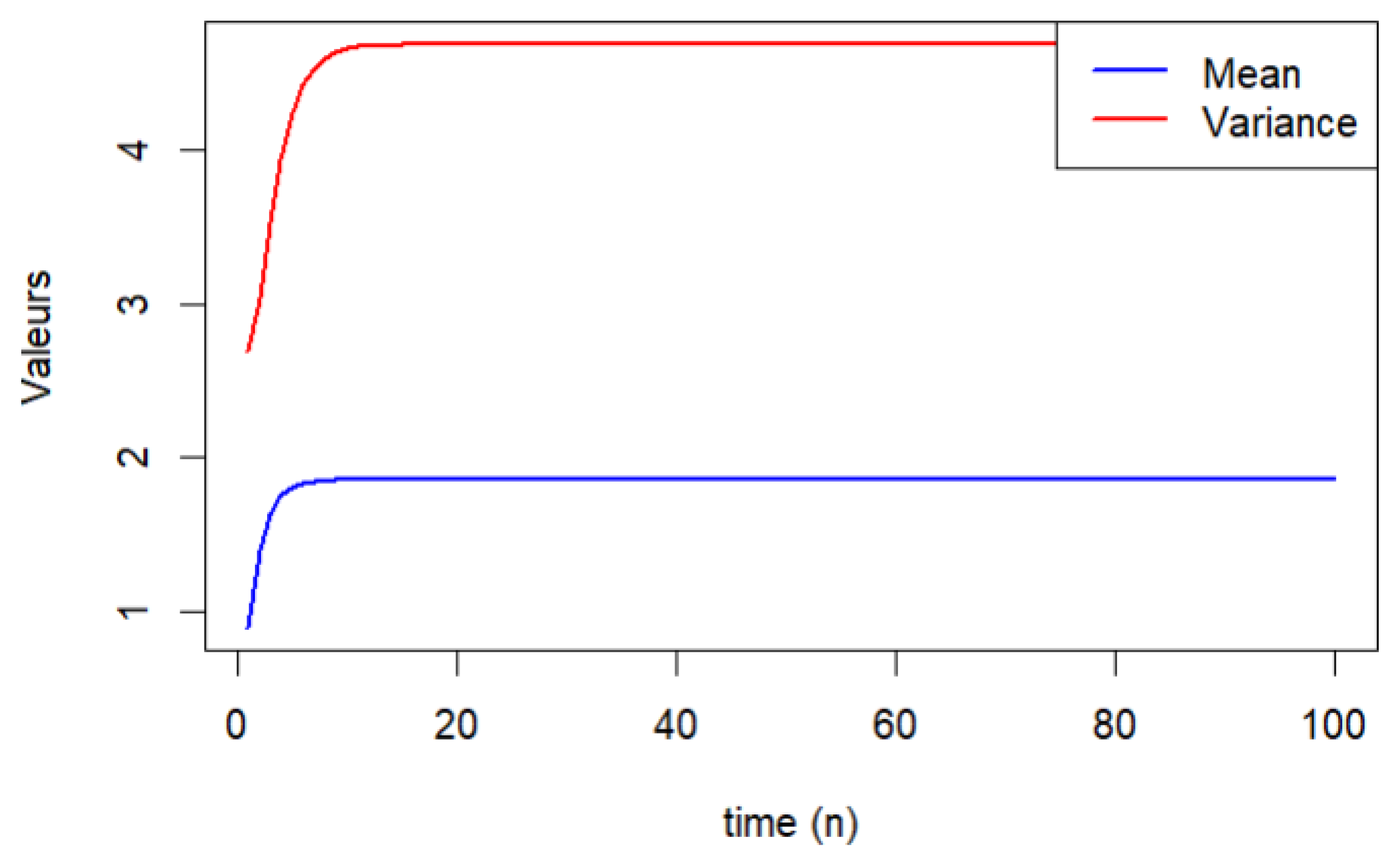
Figure 3. Curve of the mean and variance of the final altitude Z ˜ n for Case 1 parameters.
Axioms 14 00756 g003
Table 1. Mean and variance of the final altitude Z ˜ n across different times n in three different cases: p ^ , p 1 , p 2 , p 3 , p ¯ { ( 0.1 , 0.2 , 0.25 , 0.15 , 0.3 ) , ( 0.1 , 0.5 , 0.13 , 0.1 , 0.17 ) , ( 0.1 , 0.7 , 0.1 , 0.05 , 0.05 ) } .
nCase 1Case 2Case 3
E ( Z ˜ n ) V ar ( Z ˜ n ) E ( Z ˜ n ) V ar ( Z ˜ n ) E ( Z ˜ n ) V ar ( Z ˜ n )
10.9000002.6900000.9000003.8900000.9000004.690000
21.3950003.0389751.6058004.2388061.6850005.015775
31.6380003.5169562.1226104.8959772.3547505.658902
41.7533123.9330832.4862515.7654932.9169626.630567
51.8076274.2285052.7357676.7081603.3831127.889136
61.8332674.4171862.9041557.6107323.7659159.363300
71.8454344.5305983.0165208.4062044.07788910.971901
81.8512414.5962463.0909269.0678644.33059112.637591
91.8540294.6333063.1399389.5956784.53427114.294555
101.8553734.6538633.17210910.0038654.69777715.891675
151.8566084.6771993.22570010.9161015.13457022.126498
201.8566424.6782023.23211311.0890415.27191325.378529
251.8566434.6782423.23289411.1179225.31433226.799313
301.8566434.6782433.23299111.1225005.32741527.367648
351.8566434.6782433.23300411.1232075.33147427.584513
401.8566434.6782433.23300511.1233145.33274427.665079
451.8566434.6782433.23300511.1233315.33314527.694527
501.8566434.6782433.23300511.1233335.33327327.705178
1001.8566434.6782433.23300511.1233335.33333327.711111
5001.8566434.6782433.23300511.1233335.33333327.711111
10001.8566434.6782433.23300511.1233335.33333327.711111
Disclaimer/Publisher’s Note: The statements, opinions and data contained in all publications are solely those of the individual author(s) and contributor(s) and not of MDPI and/or the editor(s). MDPI and/or the editor(s) disclaim responsibility for any injury to people or property resulting from any ideas, methods, instructions or products referred to in the content.