Article

Modeling and Transmission Dynamics of a Stochastic Fractional Delay Cervical Cancer Model with Efficient Numerical Analysis

1
Department of Mathematics, National College of Business Administration and Economics, Lahore 54660, Pakistan
2
Center for Research and Development in Mathematics and Applications (CIDMA), Department of Mathematics, University of Aveiro, 3810-193 Aveiro, Portugal
3
Department of Mathematical Sciences, College of Science, Princess Nourah bint Abdulrahman University, P.O. Box 84428, Riyadh 11671, Saudi Arabia
*
Authors to whom correspondence should be addressed.
Axioms 2025, 14(10), 742; https://doi.org/10.3390/axioms14100742
Submission received: 3 July 2025 / Revised: 25 September 2025 / Accepted: 26 September 2025 / Published: 30 September 2025
(This article belongs to the Special Issue Mathematical Methods in the Applied Sciences, 2nd Edition)

Abstract

According to the World Health Organization (WHO), globally, cervical cancer ranks as the fourth most common cancer in women, with around 660,000 new cases in 2022. In the same year, about 94 percent of the 350,000 deaths caused by cervical cancer occurred in low- and middle-income countries. This paper focuses on the dynamics of HPV by modeling the interactions between four compartments, as follows: S(t), the number of susceptible females; I(t), females infected with HPV; X(t), females infected with HPV but not yet affected by cervical cancer (CCE); and V(t), females infected with HPV and affected by CCE. A compartmental model is formulated to analyze the progression of HPV, ensuring all key mathematical properties, such as existence, uniqueness, positivity, and boundedness of the solution. The equilibria of the model, such as the HPV-free equilibrium and HPV-present equilibrium, are analyzed, and the basic reproduction number, R 0 , is computed using the next-generation matrix method. Local and global stability of these equilibria are rigorously established to understand the conditions for disease eradication or persistence. Sensitivity analysis around the reproduction number is carried out using partial derivatives to identify critical parameters influencing R 0 , which gives insights into effective intervention strategies. With appropriate positivity, boundedness, and numerical stability, a new stochastic non-standard finite difference (NSFD) scheme is developed for the proposed model. A comparison analysis of solutions shows that the NSFD scheme is the most consistent and reliable method for a stochastic fractional delay model. Graphical simulations are presented to provide visual insights into the development of the disease and lend the results to a more mature discourse. This research is crucial in highlighting the mathematical rigor and practical applicability of the proposed model, contributing to the understanding and control of HPV progression.

1. Introduction

Human papillomavirus (HPV) is a leading cause of cervical cancer, particularly in low- and middle-income countries. Understanding its transmission dynamics is crucial for designing effective public health interventions. This study aims to develop a robust theoretical framework that captures the complexity of HPV transmission using a stochastic fractional delay differential model. Our objective is not only to explore the theoretical properties of the proposed model—such as existence, uniqueness, and stability—but also to assess how different parameters influence disease transmission and to simulate possible disease outcomes under varying scenarios. By combining mathematical rigor with computational simulation, this study contributes to both the theoretical understanding and potential control strategies for HPV-related cervical cancer. Various mathematical models have been proposed to study HPV transmission dynamics and its link to cervical cancer. Early deterministic models focused on compartmental structures and parameter fitting to describe disease progression [1,2,3]. With the rise of fractional calculus, researchers have introduced fractional-order models to capture memory and hereditary effects in disease dynamics, using derivatives such as the Caputo derivative or the Atangana–Baleanu derivative to reflect the long-term behavior of infections like HPV [4,5,6]. Meanwhile, stochastic approaches were developed to incorporate randomness and individual variability, offering more realistic simulations of infection spread [7,8]. Some studies also explored gender-specific transmission and the impact of interventions such as vaccination [9,10,11,12]. Reviews have discussed national and regional differences in HPV vaccine adoption, including barriers in Asia-Pacific countries [11], practical challenges in China [12], and public health implications of vaccine effectiveness [8]. Real-world investigations have also considered co-infections with other viruses [13], cervical screening strategies [14], HPV genome dynamics [15], and targeted population studies, such as women with autoimmune conditions [16] or regions with low vaccine uptake [17]. Additionally, molecular-level models have explored potential prevention and therapeutic pathways [18,19], and global mitigation strategies have been proposed to optimize vaccine programs [20]. Despite these advancements, very few studies integrate all three critical aspects: stochastic effects, fractional dynamics, and time delays, particularly tailored for HPV-driven cervical cancer models. This gap limits our ability to model real-world complexities, such as delayed immune response, uncertainty in transmission, and memory effects in infection persistence. The current study addresses this shortcoming by proposing and analyzing a stochastic fractional delay model that captures these interlinked phenomena within a unified framework. Human papillomavirus (HPV) infections are characterized by long latency periods, persistence in the host, and delayed progression to cervical cancer, often spanning months or even years. These features indicate the presence of memory and hereditary effects in the infection and immune response dynamics. Classical integer-order models assume instantaneous responses, which may oversimplify such complex biological interactions. In contrast, fractional-order derivatives offer a natural mathematical framework to model these memory effects, where the current state depends not only on the present but also on the entire history of the system. This makes fractional modeling particularly suitable for diseases like HPV, where the timing and accumulation of viral exposure play a significant role in disease progression. Therefore, adopting a fractional framework allows for a more accurate and biologically realistic representation of HPV transmission and evolution. The stochastic delayed method combines aspects of stochastic processes, fractional calculus, and temporal delays so that real-world complexity is better described. In some applications, especially in biology and economics, fractional derivatives acquire essential elements to represent that past events influence present and future planning. It is through delays that cause-and-effect relationships, having a time dependence, are realistically simulated. In addition, the stochastic component aims to cover the risks and uncertainties in systems. Together, these pieces increase model accuracy, whereupon the explanation of natural processes can be advanced in broad scientific fields. Although the model incorporates stochastic and delay elements in its formulation, the analytical results in this section focus primarily on the deterministic backbone of the system. This allows us to establish essential mathematical properties—such as existence, uniqueness, and stability—under fractional dynamics and delay, while omitting stochastic noise for tractability.
This research article is organized into six sections. Section 1 provides a critical review of the literature on human papillomavirus (HPV), focusing on its epidemiology, biological characteristics, and gaps in existing mathematical models. Section 2 recalls the fundamental definitions of fractional calculus. Our results are given in Section 3; we outline the development of the proposed model, including discussions on existence, uniqueness, positivity, boundedness, the basic reproduction number, local and global stability, and sensitivity analysis. Section 4 introduces the stochastic numerical methods used, particularly the non-standard finite difference (NSFD) scheme, and compares their properties in terms of positivity, boundedness, and stability. We end this section by presenting graphical simulations that illustrate the dynamic behavior of the model, along with detailed interpretations and real-world implications. Section 5 and Section 6 present the discussion and conclusions, summarizing the main findings, highlighting key contributions, and suggesting directions for future research.

2. Preliminaries

This section recalls the fundamental definitions that are necessary for understanding our main results.
Definition 1
(See [21]). Let q C n be a function. The Caputo fractional derivative of order α, α ( n 1 , n ) , where n N is defined as follows:
D t α 0 c q ( t ) = 1 Γ ( n α ) 0 t q ( n ) ( T ) ( t T ) α + 1 n d T .
Definition 2
(See [21]). For a given function q ( t ) , the fractional integral of order α > 0 is defined as follows:
I t α q ( t ) = 1 Γ ( α ) 0 t ( t T ) α 1 q ( T ) d T
Here, Γ ( α ) generalizes the factorial function for real and complex numbers.
Definition 3.
A function f ( t , y ) satisfies the Lipschitz condition in the variable y on the set D R 2 if there exists a constant L > 0 such that
f ( t , y 1 ) f ( t , y 2 ) L y 1 y 2
for all ( t , y 1 ) , ( t , y 2 ) D . Here, L is called the Lipschitz constant.
Definition 4.
Let ( Ω , F , P ) be a given probability space. A collection of random variables { X ( t ) , t T } defined on the probability space ( Ω , F , P ) is called a stochastic process. A stochastic process is also called a random process or a chance process, where Ω is the sample space, F is the σ-algebra, and P is a probability measure.
Definition 5.
A stochastic process { X ( t ) , t 0 } , is said to be a Brownian motion with drift μ and volatility σ if X ( t ) = μ t + σ W ( t ) where (i) W ( t ) is a standard Brownian motion, (ii) < μ < is a constant, and (iii) σ > 0 is a constant. This is a generalization of standard Brownian motion. In this process, the mean function E [ X ( t ) ] = μ t and covariance function Cov ( W ( s ) , W ( t ) ) = σ 2 min ( s , t ) ,    s , t 0 .

3. Main Results

In this part, the dynamics of the cervical cancer epidemic (CCE) due to human papillomavirus (HPV) infection are introduced. The variables S ( t ) , I ( t ) , X ( t ) , and V ( t ) represent the numbers of susceptible females, females infected with HPV, females infected with HPV but not yet affected by CCE, and females infected with HPV and affected by CCE, respectively. The order of compartments in the CCE model is presented in Figure 1, where N denotes the total number of women, β represents the probability of infection with HPV, δ represents the probability that she will have cervical cancer, and Λ , μ represent the birth rate and mortality rate of the human population, respectively. The normalized model is obtained by considering N = 1 . One of the state variables, X or V, can be canceled out because of the no-coupling effect, as shown by the block diagram in Figure 1. In this model, the parameter β represents the effective contact rate leading to HPV transmission. It captures the likelihood that a susceptible individual becomes infected after contact with an infectious person. We assume a constant β across all transitions involving infection (i.e., contacts with individuals in compartments I , X , or V). This simplification allows the model to focus on the effects of delay, stochasticity, and fractional order without introducing excessive complexity. However, we recognize that in real-world scenarios, the transmission rate may differ between early-stage infection I, latent carriers X, and individuals with cervical cancer V due to variations in viral shedding or behavior.
Human papillomavirus (HPV) is a virus that spreads in a complex way. To study it, we start with a basic mathematical model from earlier work [1]. In this study, we change the usual time derivatives to fractional Caputo derivatives of order α . This change helps to better represent how HPV spreads over time. The model shows how the infection moves through a population and helps us to understand its development, how it is passed on, and how it might be controlled. The model is given by the following system of differential equations:
D t α 0 c [ S ] = Λ α β α S ( t τ ) I ( t τ ) e μ α τ μ α S + σ 1 S d ( B ) ,
D t α 0 c [ I ] = β α S ( t τ ) I ( t τ ) e μ α τ ( δ α + μ α ) I + σ 2 I d ( B ) ,
D t α 0 c [ V ] = δ α I μ α V + σ 3 V d ( B ) .
The initial conditions for the system of Equations (1)–(3) are as follows:
S ( 0 ) = S 0 0 ,    I ( 0 ) = I 0 0 ,    V ( 0 ) = V 0 0 ,    t 0 ,    τ < t .
We assume that the state functions S ( t ) , I ( t ) , and V ( t ) are continuous on the interval [ 0 , T ] , and that their Caputo fractional derivatives of order α ( 0 , 1 ] exist and are integrable over this interval. The regularity condition required for the Caputo fractional derivative reads as follows:
D t α 0 c f ( t ) = 1 Γ ( 1 α ) 0 t f ( s ) ( t s ) α d s
where f C 1 ( [ 0 , T ] ) and, hence, the existence of the classical derivative is ensured.
This model also includes random effects that are represented by stochastic fluctuations, noted as σ i ,    i = 1 , 2 , 3 . These fluctuations are influenced by a Brownian motion B ( t ) , which is a continuous random process over time t 0 . The parameter τ < t stands for a time delay in the system, meaning the delayed influence only starts to show after some time has passed.

3.1. Existence and Uniqueness

In this section, the existence and uniqueness of the stochastic fractional delayed model are established. At the beginning, let us assume σ i = 0 ,    i = 1 , 2 , 3 , and by applying the Caputo fractional integral to the system of Equations (1)–(3), we get
S ( t ) = S 0 + 1 Γ ( α ) 0 t ( t s ) α 1 1 ( s , S ) d s ,
I ( t ) = I 0 + 1 Γ ( α ) 0 t ( t s ) α 1 2 ( s , I ) d s ,
V ( t ) = V 0 + 1 Γ ( α ) 0 t ( t s ) α 1 3 ( s , V ) d s .
The functions defined under the integral in the system of Equations (4)–(6) are
1 ( t , S ) = Λ α β α S I e μ α τ μ α S ,
2 ( t , I ) = β α S I e μ α τ ( δ α + μ α ) I ,
3 ( t , V ) = δ α I μ α V .
The initial conditions for the system of Equations (7)–(9) are as follows:
1 ( 0 ) 0 , 2 ( 0 ) 0 , 3 ( 0 ) 0 , t 0 , τ < t .
It is also assumed that E 1 ,    E 2 ,    E 3 are positive constants, and that the functions S ( t ) , I ( t ) , V ( t ) remain non-negative over time. Specifically, they satisfy the following bounds:
S ( t ) E 1 , I ( t ) E 2 , V ( t ) E 3 .
Theorem 1.
Let σ i = 0 , i = 1 , 2 , 3 , then the functions i , i = 1 , 2 , 3 , satisfy the Lipschitz condition with constants L i . If W = max { L 1 , L 2 , L 3 } < 1 is satisfied, then each i is a contraction mapping.
Proof. 
First, we analyze the Lipschitz condition for the function 1 (t,S). For this, we write S and S 1 :
1 ( t , S ) 1 ( t , S 1 ) = Λ α β α S I e μ α τ μ α S Λ α β α S 1 I e μ α τ μ α S 1 .
1 ( t , S ) 1 ( t , S 1 ) = β α I e μ α τ ( S S 1 ) + μ α ( S S 1 ) .
1 ( t , S ) 1 ( t , S 1 ) β α I e μ α τ ( S S 1 ) + μ α ( S S 1 ) .
1 ( t , S ) 1 ( t , S 1 ) β α e μ α τ I + μ α S S 1 .
1 ( t , S ) 1 ( t , S 1 ) β α e μ α τ E 2 + μ α S S 1 .
1 ( t , S ) 1 ( t , S 1 ) ξ 1 S S 1 .
In this instance, ξ 1 = β α e μ α τ E 2 + μ α . The Lipschitz condition holds. A similar approach can be applied to verify that i , i = 2 , 3 also satisfies this condition. For instance, first, we analyze the Lipschitz condition for the function 2 ( t , I ) . For this, we write the following:
2 ( t , I ) 2 ( t , I 1 ) = β α S I e μ α τ ( δ α + μ α ) I β α S I 1 e μ α τ ( δ α + μ α ) I 1 .
2 ( t , I ) 2 ( t , I 1 ) = β α S e μ α τ ( I I 1 ) + ( δ α + μ α ) ( I 1 I ) .
2 ( t , I ) 2 ( t , I 1 ) β α E 1 e μ α τ + ( δ α + μ α ) I 1 I .
2 ( t , I ) 2 ( t , I 1 ) ξ 2 I 1 I .
For ξ 2 = β α E 1 e μ α τ + ( δ α + μ α ) , a Lipschitz condition holds.
Now, we analyze the Lipschitz condition for the function 3 ( t , V ) . For this, we write the following:
3 ( t , V ) 3 ( t , V 1 ) = ( δ α I μ α V ) ( δ α I μ α V 1 ) .
3 ( t , V ) 3 ( t , V 1 ) = μ α ( V V 1 ) .
3 ( t , V ) 3 ( t , V 1 ) μ α V V 1 .
3 ( t , V ) 3 ( t , V 1 ) ξ 3 V V 1 .
For ξ 3 = μ α , a Lipschitz condition holds. Moreover, if W = max { L 1 , L 2 , L 3 } < 1 , then the functions are contraction mappings. In addition, the system of Equations (4)–(6) contains constant terms throughout:
S n ( t ) = 1 Γ ( α ) 0 t ( t s ) α 1 1 s , S n 1 d s ,
I n ( t ) = 1 Γ ( α ) 0 t ( t s ) α 1 2 s , I n 1 d s ,
V n ( t ) = 1 Γ ( α ) 0 t ( t s ) α 1 3 s , V n 1 d s .
where S ( 0 ) = S 0 0 , I ( 0 ) = I 0 0 , V ( 0 ) = V 0 0 .
The variation between the two terms is described by the following expressions in Equations (10)–(12):
ψ n ( t ) = S n ( t ) S n 1 ( t ) = 1 Γ ( α ) 0 t 1 ( s , S n 1 ) 1 ( s , S n 2 ) d s ,
ϕ n ( t ) = I n ( t ) I n 1 ( t ) = 1 Γ ( α ) 0 t 2 ( s , I n 1 ) 2 ( s , I n 2 ) d s ,
ϑ n ( t ) = V n ( t ) V n 1 ( t ) = 1 Γ ( α ) 0 t 3 ( s , V n 1 ) 3 ( s , V n 2 ) d s .
Therefore, we have
S n ( t ) = i = 0 n ψ i ( t ) ,
I n ( t ) = i = 0 n ϕ i ( t ) ,
V n ( t ) = i = 0 n ϑ i ( t ) .
Let us estimate as follows:
ψ n ( t ) = S n ( t ) S n 1 ( t ) .
ψ n ( t ) = 1 Γ ( α ) 0 t 1 ( s , S n 1 ) 1 ( s , S n 2 ) d s .
ψ n ( t ) ξ 1 Γ ( α ) 0 t S n 1 ( s ) S n 2 ( s ) d s .
ψ n ( t ) ξ 1 Γ ( α ) 0 t ψ n 1 ( s ) d s .
The remaining equations in the system of Equations (13)–(15) can be solved using a similar method, resulting in the following:
ϕ n ( t ) ξ 2 Γ ( α ) 0 t ϕ n 1 ( s ) d s .
ϑ n ( t ) ξ 3 Γ ( α ) 0 t ϑ n 1 ( s ) d s .
The result is proved. □
Theorem 2.
If there exists t > 1 such that ξ i Γ ( α ) t < 1 , i = 1 , 2 , 3 ,  then, for the model system with σ i = 0 , i = 1 , 2 , 3 ,  there exists at least one solution.
Proof. 
Since each kernel i for i = 1 , 2 , 3 satisfies the Lipschitz condition, and the functions S ( t ) , I ( t ) , V ( t ) are bounded, the following relations can be derived:
ψ n ( t ) S ( 0 ) ξ 1 t Γ ( α ) n ,
ϕ n ( t ) I ( 0 ) ξ 2 t Γ ( α ) n ,
ϑ n ( t ) V ( 0 ) ξ 3 t Γ ( α ) n ,
The estimates derived from Equations (22)–(24), in conjunction with the bounds established in (16)–(18), confirm that the sequence of approximations converges and that the functions remain within the bounded region defined by the Lipschitz condition. This guarantees the existence of a unique solution on the interval considered.
To prove part (ii), it is necessary to show that S ( t ) , I ( t ) , V ( t ) converge to the solution of the system of Equations (1)–(3). To proceed, we define the remaining terms after n iterations as A n ( t ) , B n ( t ) , C n ( t ) , respectively. Therefore,
S ( t ) S ( 0 ) = S n ( t ) A n ( t ) ,
I ( t ) I ( 0 ) = I n ( t ) B n ( t ) ,
V ( t ) V ( 0 ) = V n ( t ) C n ( t ) .
By applying the Lipschitz condition with constant ξ 1 > 0 , the remainder can be expressed as
A n ( t ) = S ( t ) S n ( t ) = i = 0 ψ i ( t ) i = 0 n ψ i ( t ) = i = n + 1 ψ i ( t )
Hence,
A n ( t ) i = n + 1 ψ i ( t ) S ( 0 ) i = n + 1 ξ 1 t Γ ( α ) i
By using the geometric series formula, we get
A n ( t ) ε 1 ξ 1 t Γ ( α ) n + 1 1 ξ 1 t Γ ( α )
For this estimation, it follows that
lim n A n ( t ) = 0 for    ξ 1 t Γ ( α ) < 1
By using the same process as for n , we get
B n ( t ) 0 ,
C n ( t ) 0 ,
As a result, a solution exists. This completes the proof. □

3.2. Positivity and Boundedness

We begin by recalling a useful lemma.
Lemma 1.
See ref. [22]. If we have a dynamical system of the form
X = f ( X ) , X R n
and X i = 0 for all i = 1 , 2 , , n , then we just need to check that f i 0 to conclude that X is always non-negative.
Theorem 3.
Given the initial conditions and assuming σ i = 0 , i = 1 , 2 , 3 , the stochastic fractional delayed model described by Equations (1)–(3) admits a positive solution in R + 3 .
Proof. 
The system must remain non-negative throughout its domain to be considered feasible under the given initial conditions. By using Lemma 1, we obtain the following: f ( 0 , I , V , t ) = Λ α 0 ,   f ( S , 0 , V , t ) = β α S I e μ α τ 0 ,   f ( M , I , 0 , t ) = δ α I 0 . Therefore, the stochastic fractional delayed model (1)–(3) admits a positive solution, provided that the initial conditions lie within the feasible region. □
Lemma 2
(See [23]). Let u ( t ) and g ( t ) be continuous, non-negative functions on the interval [ a , b ] , and let α 0 be a constant. If u ( t ) satisfies the following inequality:
u ( t ) α + a t u ( t ) g ( s ) d s
for all t [ a , b ] , then Gronwall’s inequality states that
u ( t ) α e a t g ( s ) d s ,
for all t [ a , b ] .
Theorem 4.
The system of Equations (1)–(3) evolves within the feasible region
G = ( S ( t ) , I ( t ) , V ( t ) ) R + 3 ; 0 < N ( t ) Λ α μ α , t 0 , τ < t
where N ( t ) = S ( t ) + I ( t ) + V ( t ) . The initial conditions are assumed to be bounded and non-negative, under the assumption that σ i = 0 , i = 1 , 2 , 3 .
Proof. 
The total population N ( t ) satisfies the following inequality:
D t α 0 c N ( t ) Λ α μ α N ( t )
Solving this inequality, we obtain the following:
N ( t ) Λ α μ α + N ( 0 ) Λ α μ α e μ α t
Using Gronwall’s inequality (Lemma 2),
lim t N ( t ) Λ α μ α .
Therefore, the epidemiologically feasible region for the disease dynamics is characterized by Equation (33):
G = ( S ( t ) , I ( t ) , V ( t ) ) R + 3 ; 0 < N ( t ) Λ α μ α , t 0 , τ < t .
The stochastic fractional delayed model (1)–(3) is positively invariant and epidemiologically meaningful for modeling infection transmission, as demonstrated in (33). Consequently, the system of Equations (1)–(3) remains bounded given the specified initial conditions. □

3.3. Model Equilibria and Reproduction Number

In this section, we investigate the various states of the stochastic fractional delayed model (1)–(3) that describe the dynamics of HPV infection. By analyzing the behavior of the system, we establish the model’s properties at both the HPV-free and HPV-present equilibrium states. In addition, this investigation reveals the influence of the fractional order, delays, and stochastic parameters on infection transmission and control, with the aid of different numerical techniques. Therefore,
HPV free equilibrium ( HPVFE ) = A 0 = ( S 0 , I 0 , V 0 ) = Λ α μ α , 0 , 0 .
HPV present equilibrium ( HPVPE ) = A * = ( S * , I * , V * ) .
S * = Λ α β α e μ α τ ( δ α + μ α ) μ α β α e μ α τ ( δ α + μ α ) , I * = δ α + μ α β α e μ α τ , V * = δ α I * μ α .
In epidemiology, the basic reproduction number is one of the most significant parameters. It shows whether the disease is present in the population or not. If this value is less than one, the disease cannot spread through the population, even if it is present. To estimate the basic reproduction number, we use the next-generation matrix method. The reproduction number, defined as the largest eigenvalue (or spectral radius) at the HPV-free equilibrium, is given by the following:
R 0 = β α Λ α e μ α τ μ α δ α + μ α .

3.4. Local Stability

This part examines the stability of both model equilibria, namely the HPV-free equilibrium and the HPV-present equilibrium, in the local sense.
Theorem 5.
Assuming σ i = 0 , i = 1 , 2 , 3 , the HPV-free equilibrium point given in (34) is locally asymptotically stable if α ( 0 , 1 ) and the basic reproduction number R 0 < 1 .
Proof. 
By linearizing the stochastic fractional delayed system of Equations (1)–(3) around the equilibrium point in (34), we obtain a 3 × 3 Jacobian matrix whose eigenvalues all have negative real parts, confirming local asymptotic stability:
| J A 0 λ I | = 0
μ α λ β α S 0 e μ α τ 0 0 β α S 0 e μ α τ ( δ α + μ α ) λ 0 0 δ α μ α λ = 0
λ 1 = λ 2 = μ α , λ 3 = ( δ α + μ α ) ( 1 R 0 ) .
Therefore, the HPV-free equilibrium of the stochastic fractional delayed system of Equations (1)–(3) is locally stable whenever R 0 < 1 . Conversely, if R 0 > 1 , the equilibrium given in (37) becomes locally unstable. □
Theorem 6.
Assuming σ i = 0 , i = 1 , 2 , 3 , the HPV-present equilibrium given in (35) is locally asymptotically stable for α ( 0 , 1 ) if the basic reproduction number R 0 > 1 .
Proof. 
Consider the stochastic fractional delayed system of Equations (1)–(3). By linearizing the system around the HPV-present equilibrium point given in (35), we analyze the corresponding Jacobian matrix. If all eigenvalues of this matrix have negative real parts, the equilibrium is locally asymptotically stable, which occurs when R 0 > 1 .
| J A * λ | = 0 ,
β α I * e μ α τ μ α λ β α S * e μ α τ 0 β α I * e μ α τ β α S * e μ α τ ( δ α + μ α ) λ 0 0 δ α μ α λ = 0
λ = μ α
β α I * e μ α τ μ α λ β α S * e μ α τ β α I * e μ α τ β α S * e μ α τ ( δ α + μ α ) λ = 0
a 1 λ a 2 a 3 a 4 λ = 0
( a 1 λ ) ( a 4 λ ) + a 2 a 3 = 0
λ 2 + ( a 1 + a 4 ) λ + a 1 a 4 + a 2 a 3 = 0
The corresponding second-order characteristic polynomial is given by the following:
λ 2 + A 1 λ + A 0 = 0
Here,
A 1 = a 1 + a 4 , A 0 = a 1 a 4 + a 2 a 3
a 1 = β α I * e μ α τ + μ α , a 2 = β α S * e μ α τ , a 3 = β α I * e μ α τ , a 4 = ( μ α + δ α ) β α S * e μ α τ .
The second-order characteristic polynomial has positive coefficients A 1 and A 0 . According to the Routh–Hurwitz criterion for a second-degree polynomial, the equilibrium is locally stable if these coefficients are positive, which holds when R 0 > 1 . Therefore, the HPV-present equilibrium of the system of Equations (1)–(3) is locally stable under this condition. Conversely, if R 0 < 1 , the Routh–Hurwitz stability criteria are not satisfied and, thus, equilibrium (35) is locally unstable. □

3.5. Global Stability

This part examines the stability of both model equilibria, like the HPV-free equilibrium and the HPV-present equilibrium, in the context of a global sense.
Theorem 7.
Assuming σ i = 0 , i = 1 , 2 , 3 , the stochastic fractional delayed model (1)–(3) is globally asymptotically stable (GAS) at the HPV-free equilibrium A 0 whenever R 0 < 1 .
Proof. 
Define the Volterra–Lyapunov function L : G R as follows:
L ( t ) = S S 0 S 0 log S S 0 + I + V
The Caputo fractional derivative of L ( t ) is given by
D t α 0 c L ( t ) = S S 0 S D t α 0 c S + D t α 0 c I + D t α 0 c V
= S S 0 S Λ α β α S I e μ α τ μ α S + β α S I e μ α τ ( δ α + μ α ) I + δ α I μ α V
By using the result of Equation (34), we have
D t α 0 c L ( t ) Λ α ( S S 0 ) 2 S S 0 μ α I 1 β α S e μ α τ μ α μ α V .
This implies that D t α 0 c L 0 if R 0 < 1 and D t α 0 c L = 0 if S = S 0 , I = 0 , V = 0 . Therefore, A 0 is globally asymptotically stable. □
Theorem 8.
Assuming σ i = 0 , i = 1 , 2 , 3 , the stochastic fractional delayed model (1)–(3) is globally asymptotically stable (GAS) at the HPV-present equilibrium A * when R 0 > 1 .
Proof. 
Define the Volterra–Lyapunov function Z : G R as follows:
Z = k 1 S S * S * log S S * + k 2 I I * I * log I I * + k 3 V V * V * log V V * .
Given positive constants k i ( i = 1 , 2 , 3 ) , the following equation can be written as follows:
D t α 0 c Z = k 1 ( S S * ) S D t α 0 c S + k 2 ( I I * ) I D t α 0 c I + k 3 ( V V * ) V D t α 0 c V .
D t α 0 c Z = k 1 Λ α ( S S * ) 2 S S * k 2 β α S I e μ α τ ( I I * ) 2 I I * k 3 δ α I ( V V * ) 2 V V * .
If we choose k i = 1 , ( i = 1 , 2 , 3 ) , where k i are positive constants,
D t α 0 c Z = Λ α ( S S * ) 2 S S * β α S I e μ α τ ( I I * ) 2 I I * δ α I ( V V * ) 2 V V * 0 .
D t α 0 c Z 0 , for R 0 > 1 and D t α 0 c Z = 0 if and only if the system is at the HPV-present equilibrium. According to LaSalle’s invariance principle, all trajectories that begin in the feasible region will approach this equilibrium as t . This condition ensures that the Lyapunov function decreases along trajectories and vanishes precisely at the equilibrium, confirming global asymptotic stability. □

3.6. Sensitivity Analysis

This section investigates the impact of model parameters on the basic reproduction number R 0 . Sensitivity analysis helps us to understand how changes in parameters influence the transmission and spread of the disease within the model.
The normalized sensitivity index of a variable E , which is differentiable with respect to a parameter ϱ , is defined as follows:
E ϱ E = ϱ E × E ϱ .
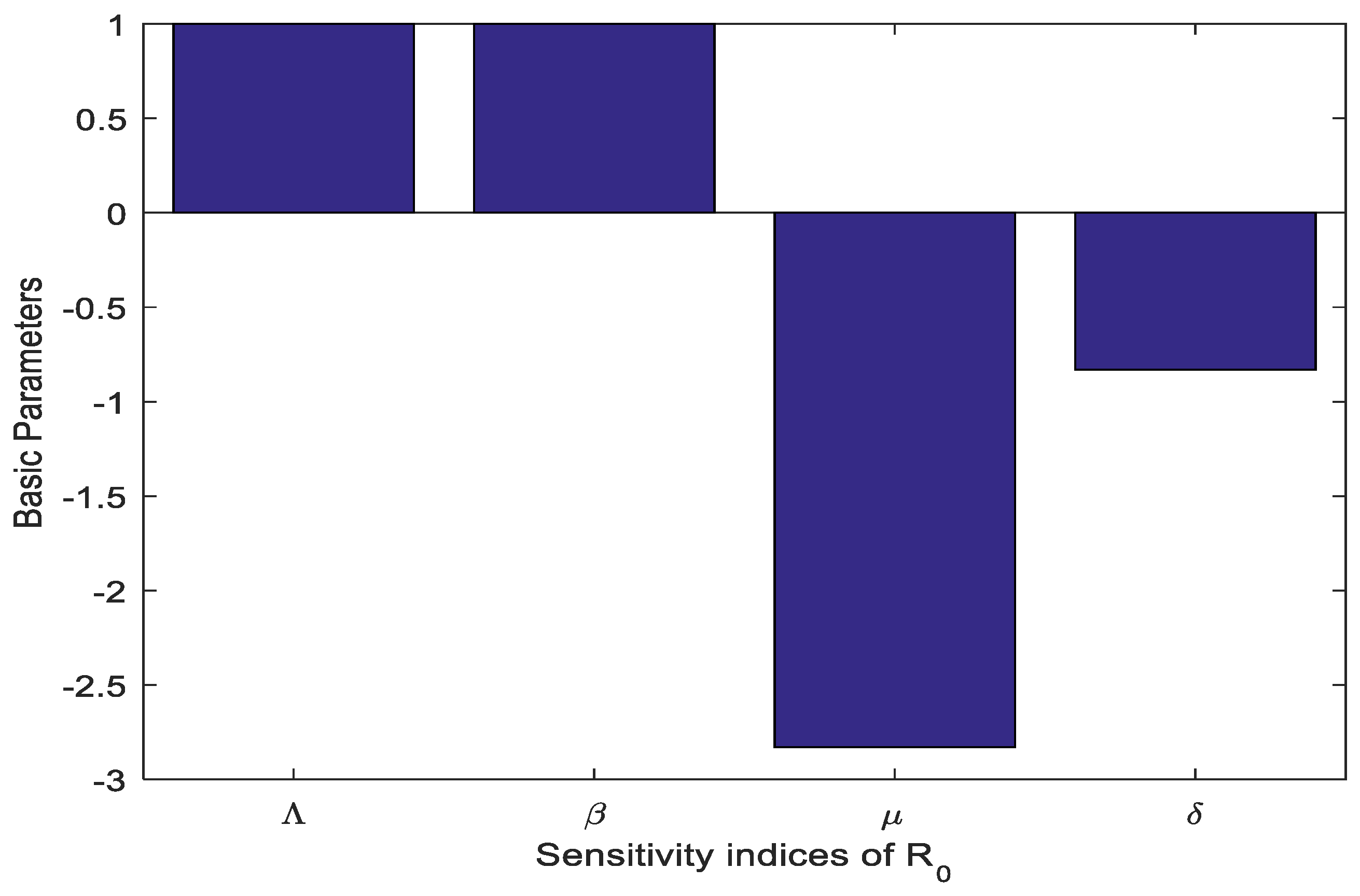
In spatial terms, we compute the sensitivity indices of the model parameters with respect to the basic reproduction number R 0 , as shown in Table 1.
To discuss the graphs for human papillomavirus (HPV), we focus on the sensitivity analysis, in particular on the reproduction number, R 0 , which is central to understanding HPV transmission dynamics. Figure 2 shows the sensitivity graph and illustrates how different parameters influence the basic reproduction number R 0 . The results include both positive and negative sensitivity indices, indicating which parameters increase R 0 as their values rise and, thus, contribute directly to HPV transmission, while others reduce R 0 as their values increase, reflecting a role in controlling or reducing disease transmission. This balance between positive and negative contributions allows researchers to identify leverage points in disease control, such as prioritizing interventions targeting highly sensitive parameters to reduce R 0 below the epidemic threshold. Table 1 classifies the parameters according to the nature of their impact on sensitivity. Positive signs signify that an increasing value enhances HPV spread; these typically correspond to variables describing transmission rates or mixing within a population. A negative sign indicates inhibition, such as the rate of recovery or the efficacy of intervention. Understanding these dynamics provides actionable insights, emphasizing the need for strategies that amplify negative sensitivity effects (e.g., by boosting recovery rates) while minimizing positive sensitivity impacts (e.g., by reducing contact rates).

4. Numerical Simulations

We introduce a generalized method for solving the stochastic fractional-order system of Equations (1)–(3) based on a stochastic non-standard finite difference (NSFD) scheme. This approach is developed using a non-local framework, as referenced in [24]. In this context, t denotes the time step size. This approach is justified to isolate and understand the fundamental dynamics introduced by fractional derivatives and delay effects. While stochastic simulations are performed in later sections, a rigorous stochastic analytical treatment is beyond the present scope and remains an important direction for future study.

4.1. Non-Standard Finite Difference (NSFD) Scheme

For the system of Equations (1)–(3), the non-standard finite difference (NSFD) scheme has the following form:
S ( n + 1 ) = S n + Δ t α Γ ( α + 1 ) Λ α + σ 1 S n Δ B 1 1 + Δ t α Γ ( α + 1 ) β α I n e μ α τ + μ α ,
I ( n + 1 ) = I n + Δ t α Γ ( α + 1 ) β α S n I n e μ α τ + σ 2 I n Δ B 2 1 + Δ t α Γ ( α + 1 ) δ α + μ α ,
V ( n + 1 ) = V n + Δ t α Γ ( α + 1 ) δ α I n + σ 3 V n Δ B 3 1 + Δ t α Γ ( α + 1 ) μ α .
Theorem 9
(Positivity). The deterministic version of the system of Equations (37)–(39) maintains the non-negativity of its solutions.
Proof. 
Since every equation in the system of Equations (37)–(39) involves only non-negative terms, starting with non-negative initial conditions ensures that the numerical solutions remain non-negative at all subsequent time steps. □
Theorem 10
(Boundedness). Assuming non-negative initial values for the system of Equations (37)–(39), there exists a constant K ( n , α ) 0 such that for every n N , the solutions satisfy the following: S n , I n , V n [ 0 , K ( n , α ) ] .
Proof. 
By summing and rearranging the equations in the numerical system of Equations (37)–(39), the following can easily be shown:
( 1 + Δ t α Γ ( α + 1 ) μ α ) S ( n + 1 ) + ( 1 + Δ t α Γ ( α + 1 ) μ α ) I ( n + 1 ) + ( 1 + Δ t α Γ ( α + 1 ) μ α ) V ( n + 1 )    ( S n + I n + V n ) + Δ t α Γ ( α + 1 ) Λ α + Δ t α Γ ( α + 1 ) σ 1 S n Δ B 1 + σ 2 I n Δ B 2 + σ 3 V n Δ B 3 .
The result is verified through mathematical induction, where K ( n + 1 , α ) represents the upper bound derived from a sequence of equations and inequalities. □
We will now move on to analyze the stability of the NSFD scheme for the system of Equations (37)–(39).
Definition 6
(See [25]). The discrete system of Equations (37)–(39) is asymptotically stable if there exist constants K 1 , K 2 , K 3 such that S ( n + 1 ) K 1 ,    I ( n + 1 ) K 2 and V ( n + 1 ) K 3    as α 1 .
Theorem 11.
Under the assumptions in Theorem 10, the system of Equations (37)–(39) is asymptotically stable.
Proof. 
This result follows directly from the conclusions established in Theorem 10. □

4.2. Graphical Simulation

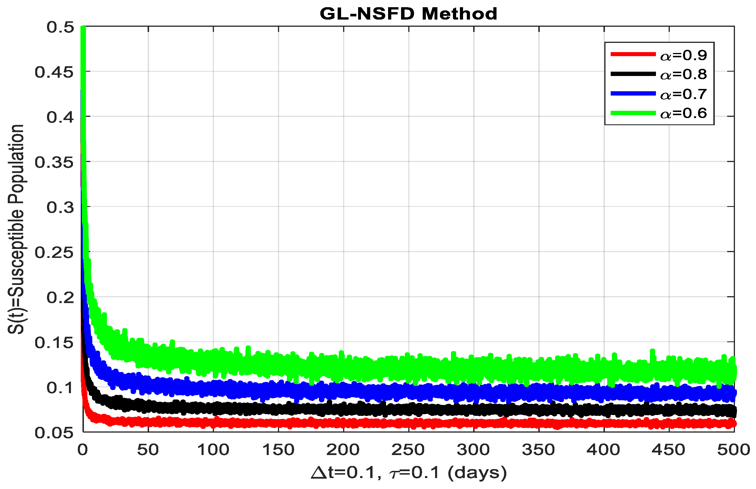
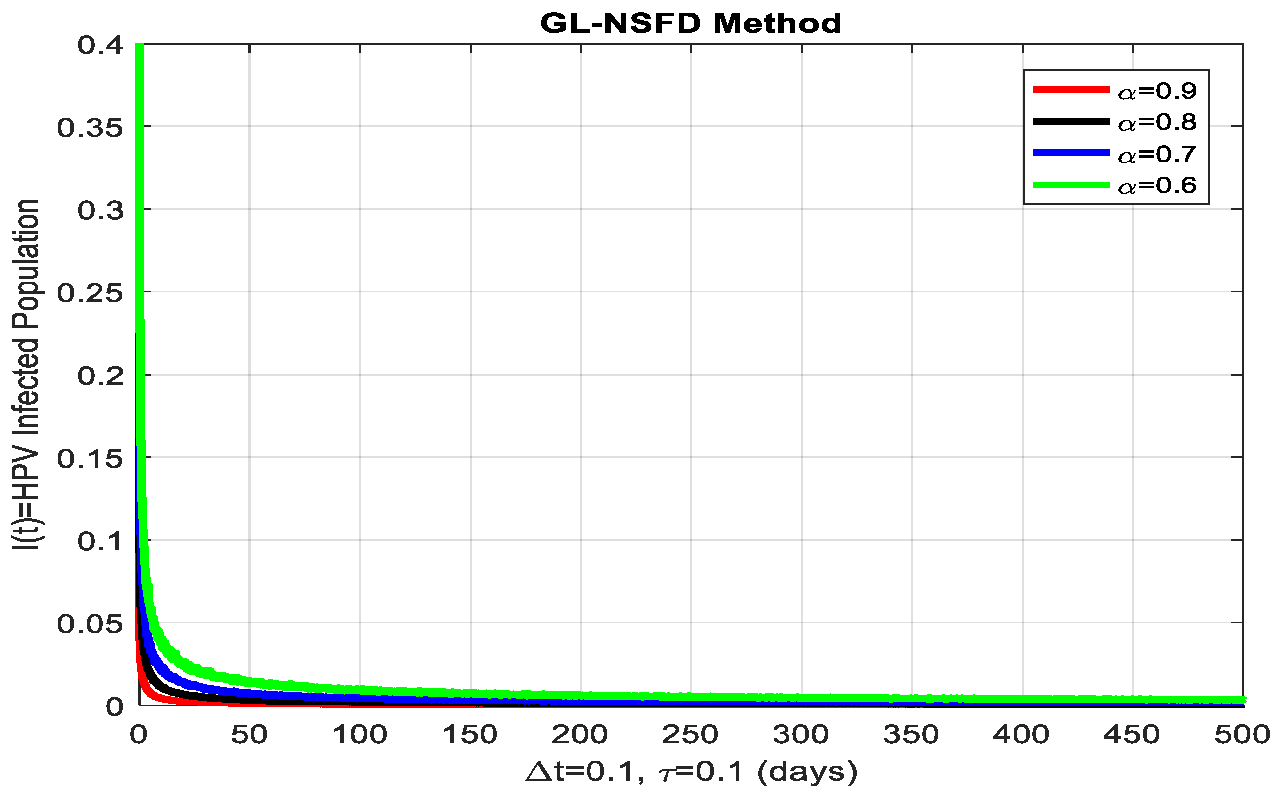
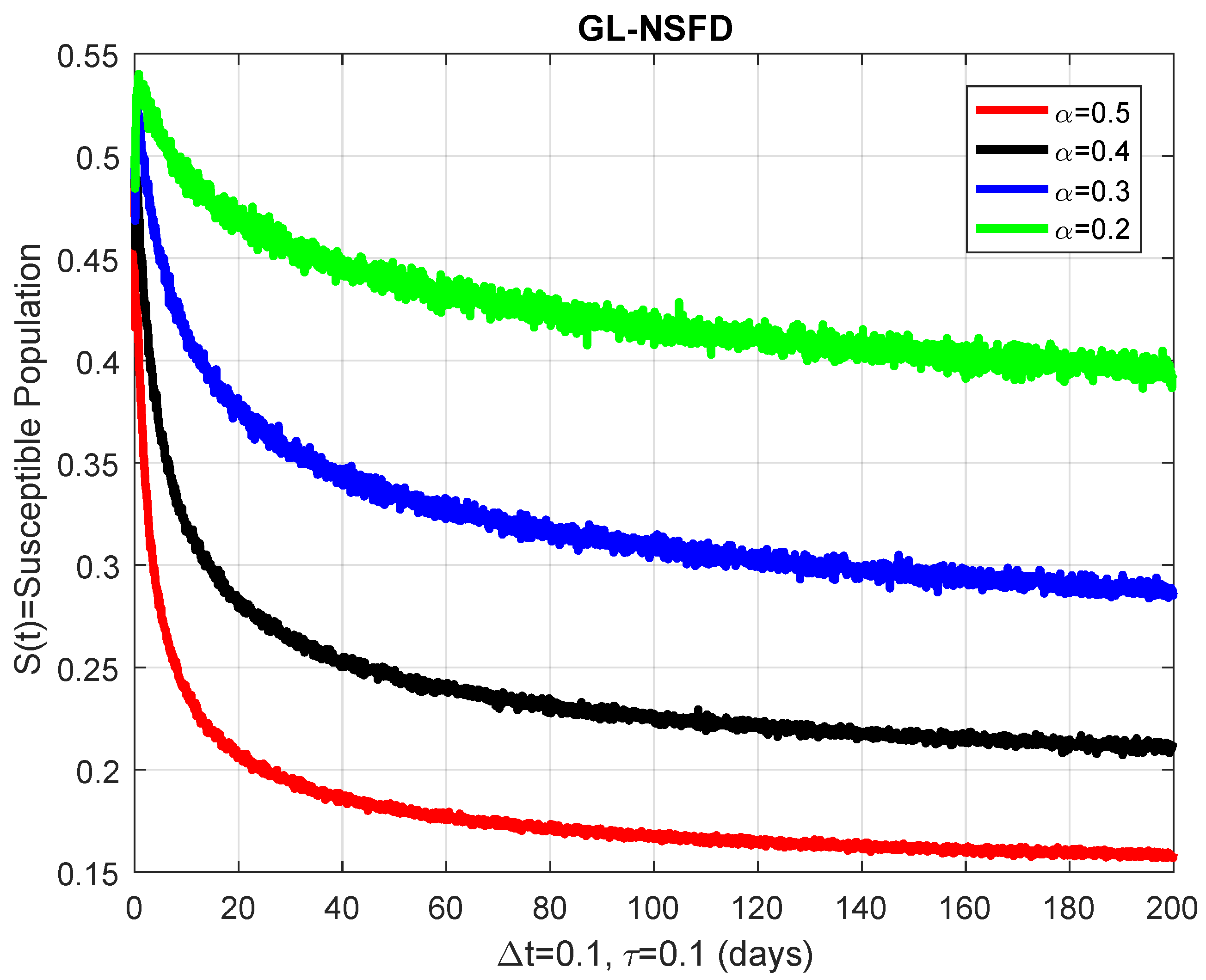
In this section, we present numerical simulations for the stochastic fractional-order model of Equations (1)–(3). The parameters used are listed in Table 2, as referenced in [1]. Figure 3, Figure 4 and Figure 5 show how each compartment in the model approaches the HPV-present equilibrium (HPV-PE). The simulations explore different values of the fractional order α , with a fixed time delay of τ = 0.1 . Each plot illustrates a distinct random path leading to the equilibrium.

5. Discussion

The graphical discussion for human papillomavirus (HPV) addresses the dynamics of disease evolution under varying values of the fractional order α , which influence the behavior of the model compartments under time-delay effects. Figure 3 and Figure 6 demonstrate that the decay in the susceptible population is slower for smaller fractional orders, meaning susceptibility lasts longer due to delays in disease progression or heterogeneity in exposure. Conversely, higher fractional orders yield a quicker reduction, closely resembling classical integer-order models in which exposure is uniform and immediate. This behavior highlights the significance of incorporating fractional dynamics to capture real-world features like immunity variability and time-lagged immune responses. It also underlines the value of early intervention strategies, such as vaccination, to reduce the long-term size of the susceptible population. Figure 4 and Figure 7 show that for lower values of α , the infected population peaks later and more extensively, indicating slower transmission and prolonged infections. In contrast, higher values produce earlier and sharper peaks, signifying faster infection cycles. These observations support the conclusion that fractional-order models better accommodate diseases with latency and memory characteristics, such as HPV. From a public health perspective, such insights are crucial. Lower α values suggest the importance of sustained treatment programs, while higher values call for rapid outbreak response strategies. Lastly, Figure 5 and Figure 8 reveal that the infectious population increases gradually and stabilizes later when α is small, illustrating delayed transmission and extended infectious periods. In contrast, higher orders show a rapid increase followed by quick stabilization, reflecting more aggressive disease spread and faster recovery. Overall, these results demonstrate that fractional-order modeling—particularly when implemented with a stable scheme like GL-NSFD—offers a powerful framework for realistically simulating complex diseases like HPV. The findings are essential for tailoring interventions to match either slow-progressing or fast-spreading disease dynamics.

6. Conclusions

In this study, the dynamics of human papillomavirus (HPV) were comprehensively analyzed through the formulation of a stochastic fractional model that incorporates all the necessary epidemiological factors. The theory of this model ensures existence, uniqueness, and positivity, together with bounded solutions. The equilibria obtained include both the HPV-free equilibrium (HPV-FE) and the HPV-present equilibrium (HPV-PE), and the reproduction number was assessed using the next-generation matrix method. The stability of the equilibria was analyzed locally and globally, and a sensitivity analysis of the reproduction number was performed using partial derivatives of key parameters that affect disease transmission. Numerical methods were used to simulate the stochastic dynamics of the model using the stochastic non-standard finite difference (NSFD) scheme, for comparison purposes at different values of the fractional order a l p h a . It demonstrated greater positivity, boundedness, and stability compared with other schemes employed for fractional-order modeling, thus affirming its high effectiveness. Theoretical findings were supported by graphical simulations, where findings about the dynamics of HPV were further understood and could be helpful for informed public health decisions. Advanced mathematical techniques, combined with numerical simulations, are necessary for understanding and predicting complex biological systems.

Author Contributions

Conceptualization, A.R. and D.F.M.T.; methodology, A.R.; software, U.S. and M.M.; validation, A.R., D.F.M.T. and M.E.A.E.; formal analysis, A.R.; investigation, A.R., D.F.M.T. and M.E.A.E.; resources, M.E.A.E.; data curation, A.R. and M.E.A.E.; writing—original draft preparation, A.R., U.S. and M.M.; writing—review and editing, D.F.M.T., U.S. and M.M.; visualization, A.R.; supervision, D.F.M.T.; project administration, A.R. and D.F.M.T.; funding acquisition, D.F.M.T. and M.E.A.E. All authors have read and agreed to the published version of the manuscript.

Funding

This work is partially supported by CIDMA under the Portuguese Foundation for Science and Technology (FCT) Multi-Annual Financing Program for R&D Units, grants UID/4106/2025 and UID/PRR/4106/2025. The authors also express their gratitude to Princess Nourah bint Abdulrahman University Researchers Supporting Project number (PNURSP2025R913), Princess Nourah bint Abdulrahman University, Riyadh, Saudi Arabia.

Data Availability Statement

The references for the data used to support the findings of this study are cited within the article.

Acknowledgments

The authors are grateful to the three anonymous referees for their comments and suggestions, which helped to improve the manuscript. The authors also express their gratitude to Princess Nourah bint Abdulrahman University Researchers Supporting Project number (PNURSP2025R913), Princess Nourah bint Abdulrahman University, Riyadh, Saudi Arabia.

Conflicts of Interest

The authors affirm that they have no conflicts of interest to declare concerning the current study.

References

  1. Ali, J.; Ciancio, A.; Khan, K.A.; Raza, N.; Baskonus, H.M.; Luqman, M.; Khan, Z.U. Evolutionary Safe Padé Approximation Scheme for Dynamical Study of Nonlinear Cervical Human Papilloma Virus Infection Model. CMES-Comput. Model. Eng. Sci. 2024, 140, 3. [Google Scholar] [CrossRef]
  2. Tivde, T.; Ameh, E.O.; Gweryina, R.I. On the Sensitivity Analysis of a Mathematical Model of the Transmission Dynamics and Control of Cervical Cancer Disease for Optimal Human Health. GSJ 2024, 12, 3. [Google Scholar]
  3. Liu, C.; Liu, H.; Zhu, X.; Lin, X. Sensitivity Analysis and Numerical Simulation of a Human Papillomavirus Infection Model. In Proceedings of the Third International Conference on Biomedical and Intelligent Systems (IC-BIS 2024), Nanchang, China, 26–28 April 2024; SPIE: Bellingham, WA, USA, 2024; Volume 13208, pp. 398–405. [Google Scholar]
  4. Bahi, M.C.; Bahramand, S.; Jan, R.; Boulaaras, S.; Ahmad, H.; Guefaifia, R. Fractional View Analysis of Sexual Transmitted Human Papilloma Virus Infection for Public Health. Sci. Rep. 2024, 14, 3048. [Google Scholar] [CrossRef]
  5. Rajan, P.K.; Kuppusamy, M.; Yusuf, A. A Fractional-Order Modeling of Human Papillomavirus Transmission and Cervical Cancer. Model. Earth Syst. Environ. 2024, 10, 1337–1357. [Google Scholar] [CrossRef]
  6. Rajan, P.K.; Kuppusamy, M. A Fractional Order Human Papillomavirus Model with Caputo Derivative. J. Anal. 2024, 32, 2135–2156. [Google Scholar] [CrossRef]
  7. Kim, M.; Kim, E. Effective Vaccination Strategies for Human Papillomavirus (HPV) Infection and Cervical Cancer Based on the Mathematical Model with a Stochastic Process. J. Med. Virol. 2024, 96, e29558. [Google Scholar] [CrossRef] [PubMed]
  8. Wang, W.; Sawleshwarkar, S.; Piraveenan, M. Computational Approaches of Modelling Human Papillomavirus Transmission and Prevention Strategies: A Systematic Review. J. Biol. Dyn. 2025, 19, 2436376. [Google Scholar] [CrossRef]
  9. Boudreau, M.C.; Cohen, J.A.; Hébert-Dufresne, L. Within-Host Infection Dynamics with Master Equations and the Method of Moments: A Case Study of Human Papillomavirus in the Epithelium. arXiv 2024, arXiv:2408.05298. [Google Scholar] [CrossRef]
  10. Cameron, R.L.; Palmer, T.J.; Cuschieri, K.; Kavanagh, K.; Roy, K. Assessing Real World Vaccine Effectiveness: A Review of Scotland’s Approach to Monitoring Human Papillomavirus (HPV) Vaccine Impact on HPV Infection and Cervical Disease. Vaccine 2024, 42, 126177. [Google Scholar] [CrossRef]
  11. Phongsamart, W.; Lou, P.J.; Sukarom, I.; Wu, Y.H.; Zaidi, O.; Du, F.; Simon, A.; Bernauer, M. Integrative Literature Review on Human Papillomavirus Vaccination Recommendations in National Immunization Programs in Select Areas in the Asia-Pacific Region. Hum. Vaccines Immunother. 2024, 20, 2362449. [Google Scholar] [CrossRef]
  12. Zhao, C.; Zhao, Y.; Li, J.; Li, M.; Shi, Y.; Wei, L. Opportunities and Challenges for Human Papillomavirus Vaccination in China. Hum. Vaccines Immunother. 2024, 20, 2329450. [Google Scholar] [CrossRef] [PubMed]
  13. Sadeghi, F.; Mostaghimi, T.; Taheri, M.; Yazdani, S.; Javadian, M.; Ranaee, M.; Ghorbani, H.; Bouzari, Z.; Sadeghi, F. Investigating the Role of Epstein-Barr Virus and Human Papillomavirus Types 16 and 18 Co-Infections in Cervical Disease of Iranian Women. Front. Oncol. 2024, 14, 1331862. [Google Scholar] [CrossRef]
  14. Wang, J.; Elfström, K.M.; Dillner, J. Human Papillomavirus-Based Cervical Screening and Long-Term Cervical Cancer Risk: A Randomised Health-Care Policy Trial in Sweden. Lancet Public Health 2024, 9, e886–e895. [Google Scholar] [CrossRef]
  15. Setayeshi, S.; Hasanzadeh, A.; Yahyapour, Y.; Alizadeh, A.; Ghorbani, H.; Nokhostin, F.; Bagheri, M.; Sadeghi, F. Evaluation of Human Papillomavirus Type 16 Viral Load and Genome Physical Status in Iranian Women with Cervical Disease. Mol. Biol. Rep. 2024, 51, 411. [Google Scholar] [CrossRef]
  16. Zhao, J.; Zhang, Z. ab0996 Human Papillomavirus Vaccination Awareness in Chinese Autoimmune Inflammatory Rheumatic Diseases: A Large Real-World Survey. Ann. Rheum. Dis. 2024, 83, 1814–1815. [Google Scholar] [CrossRef]
  17. Tobaiqy, M.; MacLure, K. A Systematic Review of Human Papillomavirus Vaccination Challenges and Strategies to Enhance Uptake. Vaccines 2024, 12, 746. [Google Scholar] [CrossRef] [PubMed]
  18. Del Prete, R.; Nesta, D.; Triggiano, F.; Lorusso, M.; Garzone, S.; Vitulano, L.; Denicolò, S.; Indraccolo, F.; Mastria, M.; Ronga, L.; et al. Human Papillomavirus Carcinogenicity and the Need of New Perspectives: Thoughts from a Retrospective Analysis on Human Papillomavirus Outcomes Conducted at the Hospital University of Bari, Apulia, Italy, between 2011 and 2022. Diagnostics 2024, 14, 968. [Google Scholar] [CrossRef]
  19. Baandrup, L.; Maltesen, T.; Dehlendorff, C.; Kjaer, S.K. Human Papillomavirus Vaccination and Anal High-Grade Precancerous Lesions and Cancer—A Real-World Effectiveness Study. JNCI J. Natl. Cancer Inst. 2024, 116, 283–287. [Google Scholar] [CrossRef]
  20. Burger, E.A.; Laprise, J.F.; Portnoy, A.; Spencer, J.C.; Sy, S.; Regan, M.C.; Kim, J.J. Population-Level Health Impact of Hypothetical Waning 1-Dose Human Papillomavirus Vaccination and 2-Dose Mitigation Strategies in a High Cervical Cancer Burden Setting. JNCI Monogr. 2024, 67, 379–386. [Google Scholar] [CrossRef] [PubMed]
  21. Albadarneh, R.B.; Batiha, I.; Alomari, A.K.; Tahat, N. Numerical Approach for Approximating the Caputo Fractional-Order Derivative Operator. AIMS Math. 2021, 6, 12743–12756. [Google Scholar] [CrossRef]
  22. Hethcote, H.W. The Mathematics of Infectious Diseases. SIAM Rev. 2000, 42, 599–653. [Google Scholar] [CrossRef]
  23. Lakshmikantham, V.; Leela, S. Differential and Integral Inequalities: Theory and Applications, Volume I: Ordinary Differential Equations; Academic Press: New York, NY, USA, 1969. [Google Scholar]
  24. Mickens, R.E. Nonstandard Finite Difference Models of Differential Equations; World Scientific: Singapore, 1993. [Google Scholar]
  25. Arenas, A.J.; Gonzalez-Parra, G.; Chen-Charpentier, B.M. Construction of Nonstandard Finite Difference Schemes for the SI and SIR Epidemic Models of Fractional Order. Math. Comput. Simul. 2016, 121, 48–63. [Google Scholar] [CrossRef]
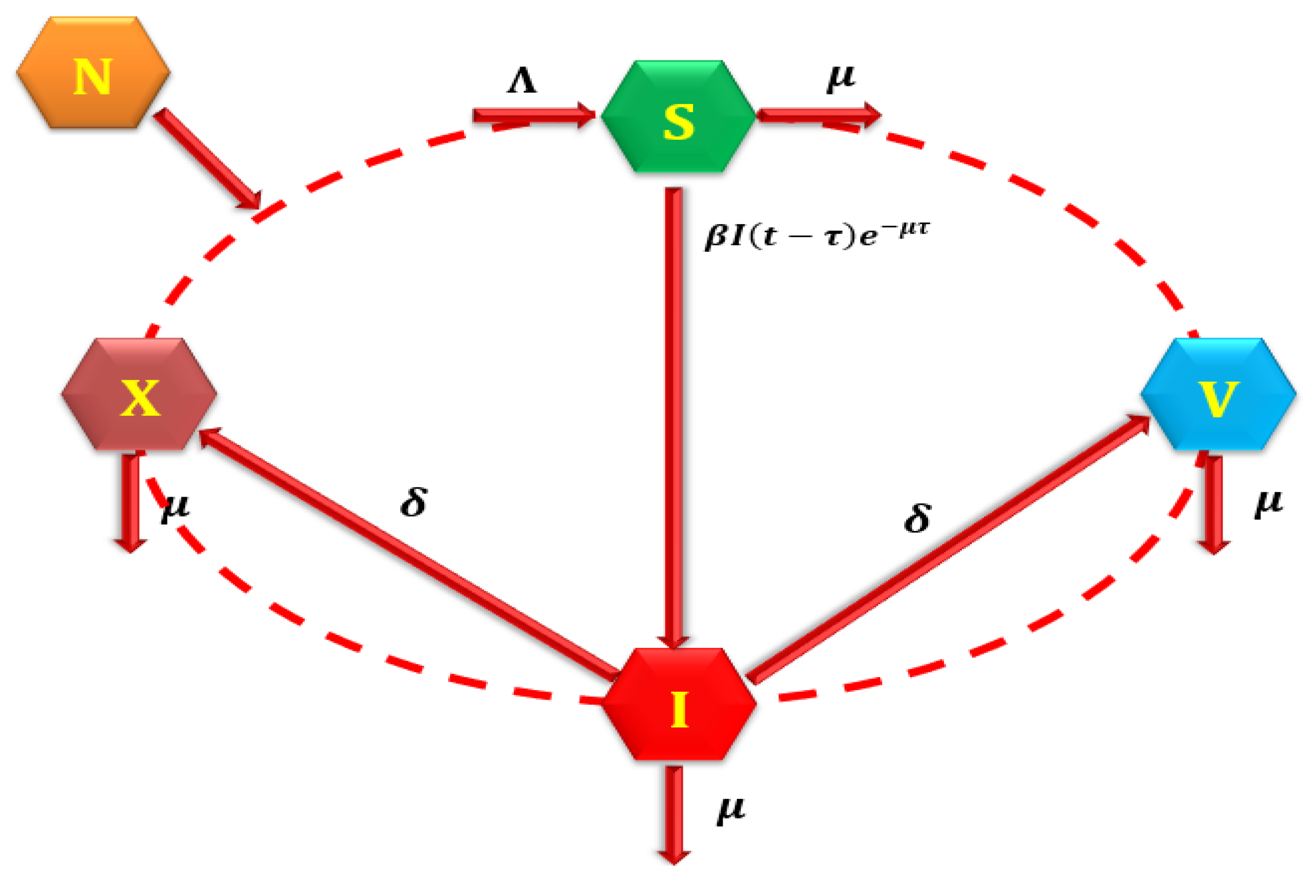
Figure 1. The compartmental structure of the model.
Axioms 14 00742 g001
Figure 2. Impact of model parameters on the reproduction number ( R 0 ) .
Axioms 14 00742 g002
Figure 3. Graphical representation of the susceptible population for various fractional-order values α .
Axioms 14 00742 g003
Figure 4. Graphical depiction of the HPV-infected population for varying fractional-order values α .
Axioms 14 00742 g004
Figure 5. Graphical illustration of the HPV infectious population across different fractional-order values α .
Axioms 14 00742 g005
Figure 6. Graphical illustration of the susceptible population for different fractional-order values α = 0.5 ,   0.4 ,   0.3 , and 0.2 .
Axioms 14 00742 g006
Figure 7. Graphical illustration of the HPV Infected population for different fractional-order values α = 0.5 ,   0.4 ,   0.3 , and 0.2 .
Axioms 14 00742 g007
Figure 8. Graphical illustration of the HPV-Infectious population for different fractional-order values α = 0.5 ,   0.4 ,   0.3 , and 0.2 .
Axioms 14 00742 g008
Table 1. Positive and negative effects of parameters.
ParametersSignsValues
Λ α Positive1.0
β α Positive1.0
δ α Negative−0.83
μ α Negative−2.83
Table 2. Description, values, and possible ranges of model parameters.
ParameterDescriptionValueRangeJustification
Λ Recruitment rate0.5[0.3, 0.7]Estimated to reflect moderate population inflow
β HPV transmission rate1.6[1.0, 2.5]Based on contact rate and infection probability [1]
μ Natural death rate0.5[0.4, 0.6]Assumed average human mortality per time unit
δ Progression rate to cervical cancer0.7[0.5, 1.0]Assumed based on typical HPV-to-CCE progression
σ i Fractional effect/intervention 0 σ i 1 [0, 1]Estimated to model intervention or memory effects
Disclaimer/Publisher’s Note: The statements, opinions and data contained in all publications are solely those of the individual author(s) and contributor(s) and not of MDPI and/or the editor(s). MDPI and/or the editor(s) disclaim responsibility for any injury to people or property resulting from any ideas, methods, instructions or products referred to in the content.