Nonparametric Density Estimation in a Mixed Model Using Wavelets

Abstract

This paper investigates nonparametric estimations of a density function within a mixed density model. A linear wavelet density estimator and an adaptive nonlinear wavelet estimator are proposed using wavelet method and hard thresholding algorithm. Under some mild conditions, the convergence rates over the mean integrated squared error of two wavelet density estimators are proved. Compared with the optimal convergence rates of nonparametric wavelet estimations, those two wavelet estimators all are optimal in some cases. Finally, the performances of two wavelet estimators are verified by numerical experimental studies.

1. Introduction

In this paper, we investigate a mixed density model as follows. The random vectors $X_1,X_2,\dots ,X_n$ are independent and identically distributed, and share a same density $g(\mathit{x})$ satisfying

$$g(\mathit{x})=\theta h(\mathit{x})+(1-\theta )f(\mathit{x}),\mathit{x}\in \Omega .$$

(1)

In the above equation, $\Omega$ is a compact support subset of ${\mathbb{R}}^d$, and $\theta$ is a known mixture parameter, $\theta \in (0,1)$. Both $h(\mathit{x})$ and $f(\mathit{x})$ are bounded densities. The model aims to recover the unknown density $f(\mathit{x})$ using the observed sample ${\left\{X_i\right\}}_{i=1}^n$.

This mixed density model has many practical applications. In the contamination problem [1,2], the density function $f(\mathit{x})$ standing for a reasonable assumption distribution is contaminated by an arbitrary assumption $h(\mathit{x})$. In addition, this model is also widely used in microarray analysis [3,4,5], neuroimaging [6] and other testing problems [7,8]. During the multiple testing, Efron et al. [9] used the above mixed model to estimate the local false discovery rate.

For the density estimation problem (1), significant results have been established through various methods, including the kernel method, maximum likelihood estimation, and polynomial techniques. Olkin and Spiegelman [10] estimated the mixture parameter $\theta$ by the maximum likelihood method, and proposed a kernel density estimator of the true density function $f(\mathit{x})$. Priebe and Marchette [11] proposed using parameter estimates as weights for kernel density estimation. James et al. [12] constructed a semiparametric density estimator, and studied the almost sure convergence rate of this estimator under some mild conditions. Robin et al. [13] estimated the unknown density function employing a weighted kernel function and adaptively selected the weights. The pointwise quadratic risk for the randomly weighted kernel estimator mentioned above was derived by [14], assuming the unknown density function pertains to a Hölder class. The convergence rates and asymptotic behavior of the density estimator were derived by [15], considering the cases of a known and an unknown mixture parameter, respectively. Deb et al. [16] proposed likelihood based methods for estimating the distribution function of the density function $f(\mathit{x})$, and discussed the statistical and computational properties of this method. To the best of our knowledge, there is no paper focus on wavelet method for estimating the unknown density function $f(\mathit{x})$.

This paper focuses on developing wavelet-based methods to address the density estimation problem (1). Wavelet has an important and satisfactory property of local time–frequency analysis. Due to this unique property, wavelet estimator can choose suitable scale parameters for estimating functions which have different functional properties in different intervals. Wavelet methods are now a staple tool in nonparametric statistics; see [17,18,19,20,21,22]. In this paper, a linear wavelet density estimator is initially introduced via the wavelet projector approach. It is noteworthy that this linear estimator exhibits unbiasedness. A convergence rate of the linear estimator over $L^2$-risk is proved in Besov spaces. Although it achieves the optimal convergence rate typical of nonparametric wavelet estimation, this linear estimator lacks adaptability. Secondly, a nonlinear wavelet estimator is derived using the hard thresholding method, which is an adaptive density estimator. Compared to its linear estimator, the nonlinear estimator achieves a superior convergence rate when $1\le p<2$. To conclude, a series of numerical experiments are provided to study the performances of those two wavelet estimators.

The rest of the paper proceeds as follows. Section 2 will provide the definitions of two wavelet density estimators and the convergence rates of those two estimators under $L^2$-risk. The performances of two wavelet estimators are studied through numerical experiments in Section 3. The proof of the main results and some auxiliary results are presented in Section 4.

2. Wavelet Estimators and Main Results

This work investigates wavelet-based density estimation for mixed models within Besov spaces. Let us first review several fundamental concepts in wavelet theory. The orthogonal multiresolution analysis (MRA) [23] defines a sequence of nested and closed linear subspaces $V_j\subset V_{j+1}$, which belong to the space of squared integrable functions $L^2({\mathbb{R}}^d)$ for any $j\in \mathbb{Z}$,

(i)

$\bigcap V_j=\left\{0\right\}$, $\overline{\bigcup V_j}=L^2({\mathbb{R}}^d);$

(ii)

$f(\mathit{x})\in V_0$ if and only if $f(2^j\mathit{x})\in V_j;$

(iii)

There exists a function $\Phi (\mathit{x})\in V_0$ for which the set $\{\Phi (\mathit{x}-\kappa )\mid \kappa \in {\mathbb{Z}}^d\}$ forms an orthonormal basis of $V_0$.

Given an orthonormal scaling function $\Phi$, the corresponding wavelets are denoted by ${\Psi }_{\mu }$ for $\mu \in 0,1,\dots ,2^d-1$. Then $S=\{{\Phi }_{\varrho ,\kappa }:=2^{\varrho d/2}\Phi (2^{\varrho }\mathit{x}-\kappa ),{\Psi }_{j,\kappa ,\mu }:=2^{jd/2}{\Psi }_{\mu }(2^j\mathit{x}-\kappa ),j\ge \varrho ,\kappa \in {\Lambda }_j\}$ form an orthonormal basis of $L^2(\Omega )$. For every integer $j_0\ge \varrho$, the function $f(\mathit{x})\in L^2(\Omega )$ can be represented by S in the following wavelet series:

$$f(\mathit{x})=\sum _{\kappa \in {\Lambda }_{j_0}}{a}_{j_0,\kappa }{\Phi }_{j_0,\kappa }(\mathit{x})+\sum _{j=j_0}^{\infty }\sum _{\mu =1}^{2^d-1}\sum _{\kappa \in {\Lambda }_j}{b}_{j,\kappa ,\mu }{\Psi }_{j,\kappa ,\mu }(\mathit{x}).$$

(2)

In this equation, ${\Lambda }_j=\{0,1,\dots ,2^{jd}-1\}$, $a_{j,\kappa }={\langle f,{\Phi }_{j,\kappa }\rangle }_{L^2(\Omega )}$, $b_{j,\kappa ,\mu }={\langle f,{\Psi }_{j,\kappa ,\mu }\rangle }_{L^2(\Omega )}$.

Let ${\mathrm{P}}_{Vj}$ denote the orthogonal projection operator from $L^2(\Omega )$ onto the subspace $V_j$. Then, for any $f(\mathit{x})\in L^2(\Omega )$,

$${\mathrm{P}}_{V_j}f(\mathit{x})=\sum _{\kappa \in {\Lambda }_j}{a}_{j,\kappa }{\Phi }_{j,\kappa }(\mathit{x}).$$

(3)

For nonparametric density estimations based on wavelet methods, it is very common to assume that the unknown density function belong to Besov spaces. It is generally acknowledged that Besov spaces are very general function spaces and can be characterized simply in terms of wavelet coefficients. Following [23], we next define Besov spaces via their wavelet coefficient characterization.

Lemma 1. 

Suppose the scale function Φ is regular of order ω, $0<s<\omega$, let $f\in L^2(\Omega )$, $1\le p,q<\infty$, the following statements are thus logically equivalent:

(i) 

$f\in B_{p,q}^s(\Omega );$

(ii) 

$\left\{2^{js}{\parallel f-{\mathrm{P}}_{V_j}f\parallel }_p\right\}\in l_q;$

(iii) 

$\{2^{j(s+\frac{d}{2}-\frac{d}{p})}{\parallel b_{j,\kappa ,\mu }\parallel }_p\}\in l_q$.

One can characterize the Besov norm of f as follows:

$${∥f∥}_{B_{p,q}^s}:={∥\left(a_{\varrho ,\kappa }\right)∥}_p+{∥{(2^{j(s+\frac{d}{2}-\frac{d}{p})}{\parallel b_{j,\kappa ,\mu }\parallel }_p)}_{j\ge \varrho }∥}_q$$

with ${∥b_{j,\kappa ,\mu }∥}_p^p={\displaystyle \sum _{\mu =1}^{2^d-1}\sum _{\kappa \in {\Lambda }_j}}{\left|b_{j,\kappa ,\mu }\right|}^p$.

We now introduce the linear wavelet estimator as follows

$${\widehat{f}}_n^{\mathrm{lin}}(\mathit{x}):=\sum _{\kappa \in {\Lambda }_{j_0}}{\widehat{a}}_{j_0,\kappa }{\Phi }_{j_0,\kappa }(\mathit{x}).$$

(4)

In the above definition,

$${\widehat{a}}_{j,\kappa }:=\frac{1}{n}\sum _{i=1}^n\frac{1}{1-\theta }{\Phi }_{j,\kappa }(X_i)-{\gamma }_{j,\kappa }$$

(5)

and ${\gamma }_{j,\kappa }={\int }_{\Omega }\frac{\theta }{1-\theta }h(\mathit{x}){\Phi }_{j,\kappa }(\mathit{x})d\mathit{x}$. In these definitions, $\theta$ stands for a known mixture parameter of the model (1). For the scale function $\Phi (\mathit{x})$, this paper uses the Daubechies wavelets [24]. It is well known that the simplest of these is the Haar wavelet. The corresponding scale functions of Daubechies wavelets can be obtained by a iterative scheme with Haar scale function [24,25]. Next, we derive the convergence rate of the linear wavelet estimator, using the notation: $x_{+}:=max\left\{x,0\right\}$. There exists a constant $c>0$, $u\lesssim v$ denotes $u\le cv$; $u\gtrsim v$ denotes $v\lesssim u$; and $u\sim v$ denotes both $u\lesssim v$ and $v\lesssim u$.

Theorem 1. 

Consider the model (1), $f(\mathit{x})\in B_{p,q}^s(\Omega )$, where $p,q\in [1,\infty )$, $s>\frac{d}{p}$. Define the linear wavelet estimator ${\widehat{f}}_n^{\mathrm{lin}}(\mathit{x})$ by (4), taking $2^{j_0}\sim n^{\frac{1}{2s^{\prime }+d}}$ where $s^{\prime }=s-d{(\frac{1}{p}-\frac{1}{2})}_{+}$, then

$$\begin{array}{c}\mathrm{E}[\parallel {\widehat{f}}_n^{\mathrm{lin}}(\mathit{x})-f(\mathit{x}){\parallel }_2^2]\lesssim n^{-\frac{2s^{\prime }}{2s^{\prime }+d}}.\end{array}$$

Remark 1. 

When $p\ge 2$, the convergence rate $(n^{-\frac{2s}{2s+d}})$ of the linear wavelet estimator ${\widehat{f}}_n^{\mathrm{lin}}(\mathit{x})$ matches the optimal convergence rate [26] for standard nonparametric wavelet estimation problems.

Compared with the optimal convergence rate $n^{-\frac{2s}{2s+d}}$ [26], the linear wavelet estimator results in a lower convergence rate in the case of $1\le p<2$. Moreover, the definition of the linear wavelet estimator ${\widehat{f}}_n^{\mathrm{lin}}(\mathit{x})$ requires knowledge of the smoothness parameter s of the unknown density $f(\mathit{x})$. However, the smoothness parameter s of the density function is usually unknown in many practical applications. As a result, this linear wavelet estimator is not adaptive. In order to overcome those shortages of the linear estimator, this paper employs a hard thresholding method to construct a nonlinear wavelet estimator.

We establish the following nonlinear wavelet estimator

$${\widehat{f}}_n^{\mathrm{non}}(\mathit{x}):=\sum _{\kappa \in {\Lambda }_{j_0}}{\widehat{a}}_{j_0,\kappa }{\Phi }_{j_0,\kappa }(\mathit{x})+\sum _{j=j_0}^{j_2}\sum _{\mu =1}^{2^d-1}\sum _{\kappa \in {\Lambda }_j}{\widehat{b}}_{j,\kappa ,\mu }{\mathbb{I}}_{\{|{\widehat{b}}_{j,\kappa ,\mu }|\ge \tau r_n\}}{\Psi }_{j,\kappa ,\mu }(\mathit{x}).$$

(6)

In this equation,

$${\widehat{b}}_{j,\kappa ,\mu }:=\frac{1}{n}\sum _{i=1}^n\frac{1}{1-\theta }{\Psi }_{j,\kappa ,\mu }(X_i)-{\vartheta }_{j,\kappa ,\mu }$$

(7)

and ${\vartheta }_{j,\kappa ,\mu }={\int }_{\Omega }\frac{\theta }{1-\theta }h(\mathit{x}){\Psi }_{j,\kappa ,\mu }(\mathit{x})d\mathit{x}$. Then, the wavelet function $\Psi (\mathit{x})$ can be constructed by the scaling relation and the scale function $\Phi (\mathit{x})$. For more details, we can refer to [24,25]. Here, the function ${\mathbb{I}}_G$ is an indicator function on G and $r_n=\sqrt{\frac{lnn}{n}}$. The convergence rate of this nonlinear wavelet estimator is presented as follows.

Theorem 2. 

Consider the model (1), $f(\mathit{x})\in B_{p,q}^s(\Omega )$, where $p,q\in [1,\infty )$, $s>\frac{d}{p}$. The nonlinear estimator ${\widehat{f}}_n^{\mathrm{non}}(\mathit{x})$ is constructed by (6) together with $2^{j_0}\sim n^{\frac{1}{2\omega +d}}(\omega >s)$, $2^{j_2}\sim {(\frac{n}{lnn})}^{\frac{1}{d}}$; then

$$\begin{array}{c}\mathrm{E}[\parallel {\widehat{f}}_n^{\mathrm{non}}(\mathit{x})-f(\mathit{x}){\parallel }_2^2]\lesssim (lnn)n^{-\frac{2s}{2s+d}}.\end{array}$$

Remark 2. 

Note that the convergence rate of this nonlinear wavelet estimator matches the optimal convergence rate $n^{-\frac{2s}{2s+d}}$ up to the $lnn$ factor.

Remark 3. 

Unlike linear estimators, both attain optimal rates for $p\ge 2$. However, the nonlinear wavelet estimator gets better convergence rate when $1\le p<2$. More importantly, the definition of the nonlinear estimator is independent of the smoothness parameter of the unknown density function, making the wavelet estimator adaptive.

Remark 4. 

According to the model (1), we can easily to see that the density function $f(\mathit{x})$ has a compact support Ω on ${\mathbb{R}}^d$. It should be pointed out that this compact support property play a important role in the definitions of two wavelet estimators and the proof of two theorems. For details, in the definitions of two wavelet estimators, $\kappa \in {\Lambda }_{j_0}$ and $\kappa \in {\Lambda }_j$ rely on the compact support property. Then the cardinalities of ${\Lambda }_{j_0}$ and ${\Lambda }_j$ satisfy $|{\Lambda }_{j_0}|\sim 2^{j_{0}d}$ and $|{\Lambda }_j|\sim 2^{jd}$, respectively. These results are used in some steps of the proofs of the two theorems, such as (12), (13), (27) and so on. Hence, similar to the classical and important work of Donoho et al. [26], this paper considers the nonparametric estimation of density function with compact support condition. On the other hand, for the nonparametric density estimation with non-compact support assumption, some significant stidoes have been conducted by [27,28].

3. Numerical Experiments

This section presents numerical experiments using R2024 software to delve into the effect of approximation of the linear and nonlinear wavelet estimators. During the experiments, the density function $f(\mathit{x})$ is estimated from the observed data set ${\left\{X_i\right\}}_{i=1}^n$. Because during the definitions of those two wavelet estimators the scale parameters $j_0$ and $j_1$ are related to the sample size n, we choose the sample size $n=4096$ in the following simulation studies. In the model (1), the mixture parameter $\theta$ is selected to be $\theta =0.025$. To assess the performance of both estimators, we adopt the mean square error (MSE) as the evaluation criterion, i.e., $\mathrm{MSE}(f,\widehat{f})=\frac{1}{n}{\displaystyle \sum _{i=1}^n}{(f(x_i)-\widehat{f}(x_i))}^2$, which is a classical and effective evaluation method in nonparametric estimations.

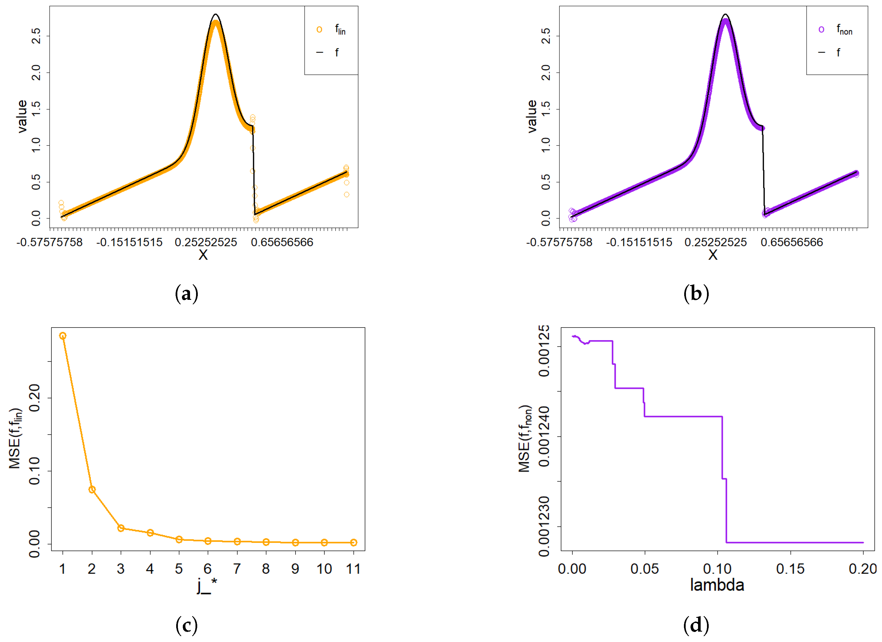
Based on the definition of linear wavelet estimator, we construct a set of linear estimators ${\widehat{f}}_n^{\mathrm{lin}}(\mathit{x})$ with different scales $j_0=0,1,\dots ,lo{g}_2(n)-1$. During the following simulation studies, we use $j_{-}^{\ast }$ to stand for the scale parameter $j_0$, which means that $j_{-}^{\ast }=j_0$. By minimizing the mean square error, we can obtain the best linear wavelet estimator with the optimal scale parameters $j_0$. For example, in the Example 1, the MSE results of the linear wavelet estimator with different scale parameter $j_0$ are shown in Figure 1c. Then, it is easy to see that the MSE of linear wavelet estimator is least when the scale parameter $j_0$ is 5, 6, 7, 8, 9 and 10. For simplicity and high efficiency, we choose the minimum scale parameter value 5, i.e., $j_0=5$.

The nonlinear estimator, according to the definition (6), has two scale parameters, $j_0$ and $j_1$. For the first scale parameter, we used the same optimal parameter $j_0$ as for the linear estimator. The other scale parameter $j_1$ is set at the maximum level permitted in the wavelet decomposition (i.e., $j_2=lo{g}_2(n)-1$ with $n=4096$). In addition, the optimal thresholding parameter $\lambda (\lambda =\tau r_n)$ is selected by minimizing the mean square error of the nonlinear wavelet estimator. For example, in the Example 1, the two scale parameters of nonlinear wavelet estimator are $j_0=5$ and $j_2=11$. On the other hand, the MSE of nonlinear wavelet estimator with different thresholding values are shown in Figure 1d. Then we can select the optimal thresholding parameter $\lambda =0.0321070234$. According to the model (1), six different functions will be selected as the density function $f(\mathit{x})$ in the following simulation study.

Example 1. 

In model (1), we take the density to be $f_1(x)=8(4x-2)e^{-{(4x-2)}^2}$. The density function $h(x)=0.57+0.5x^2+0.3cos(2x)$ and $x\in [0.5, 1.5]$. The performance of both linear and nonlinear wavelet estimators is illustrated in Figure 1a,b, respectively. As can be observed, each estimator provides an effective approximation of the density function $f(x)$. As clearly shown in Figure 1c, the optimal scale parameter is $j_0=5$. The optimal threshold parameter $\lambda =0.0321070234$ is depicted in Figure 1d.

Example 2. 

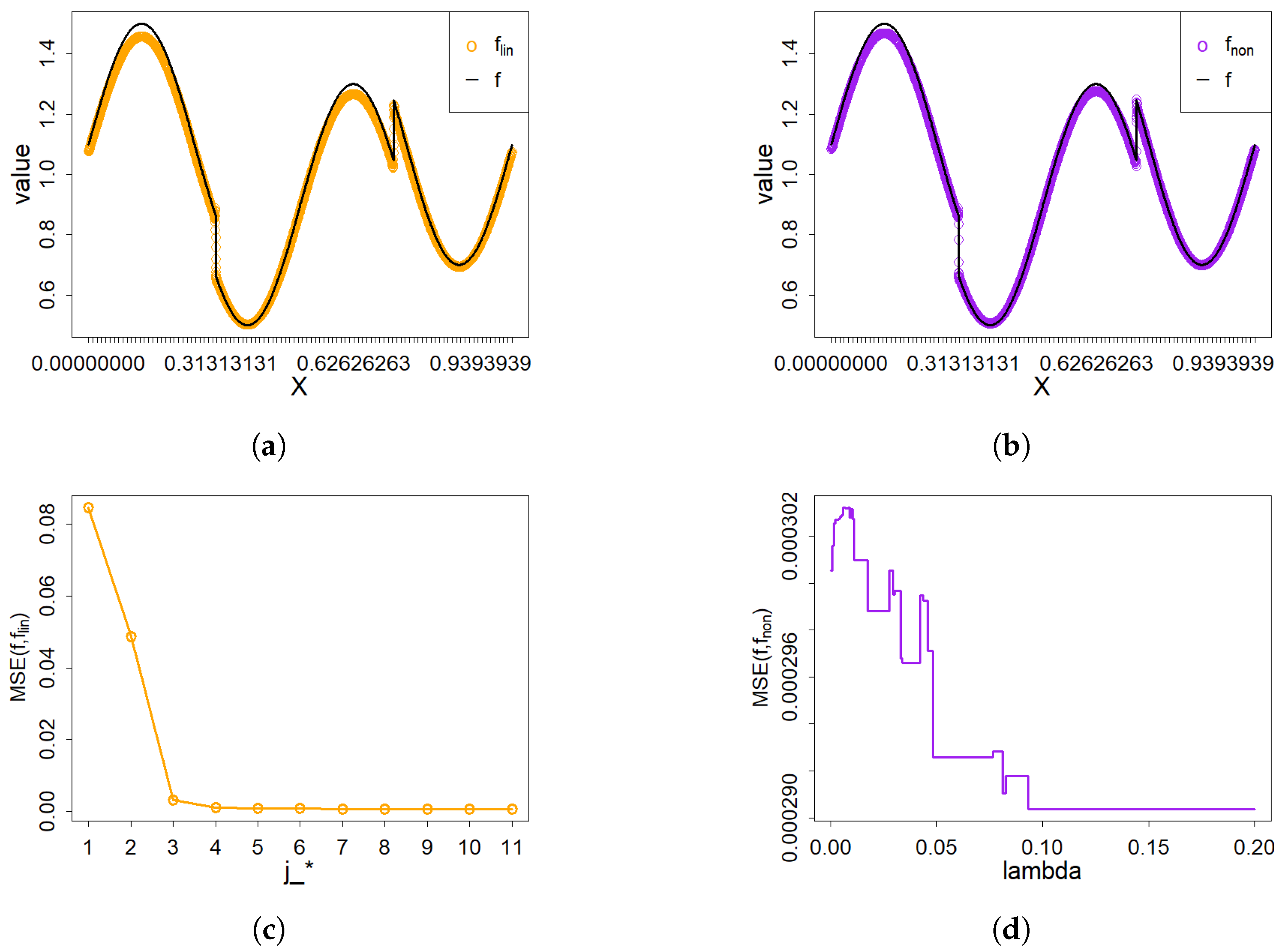
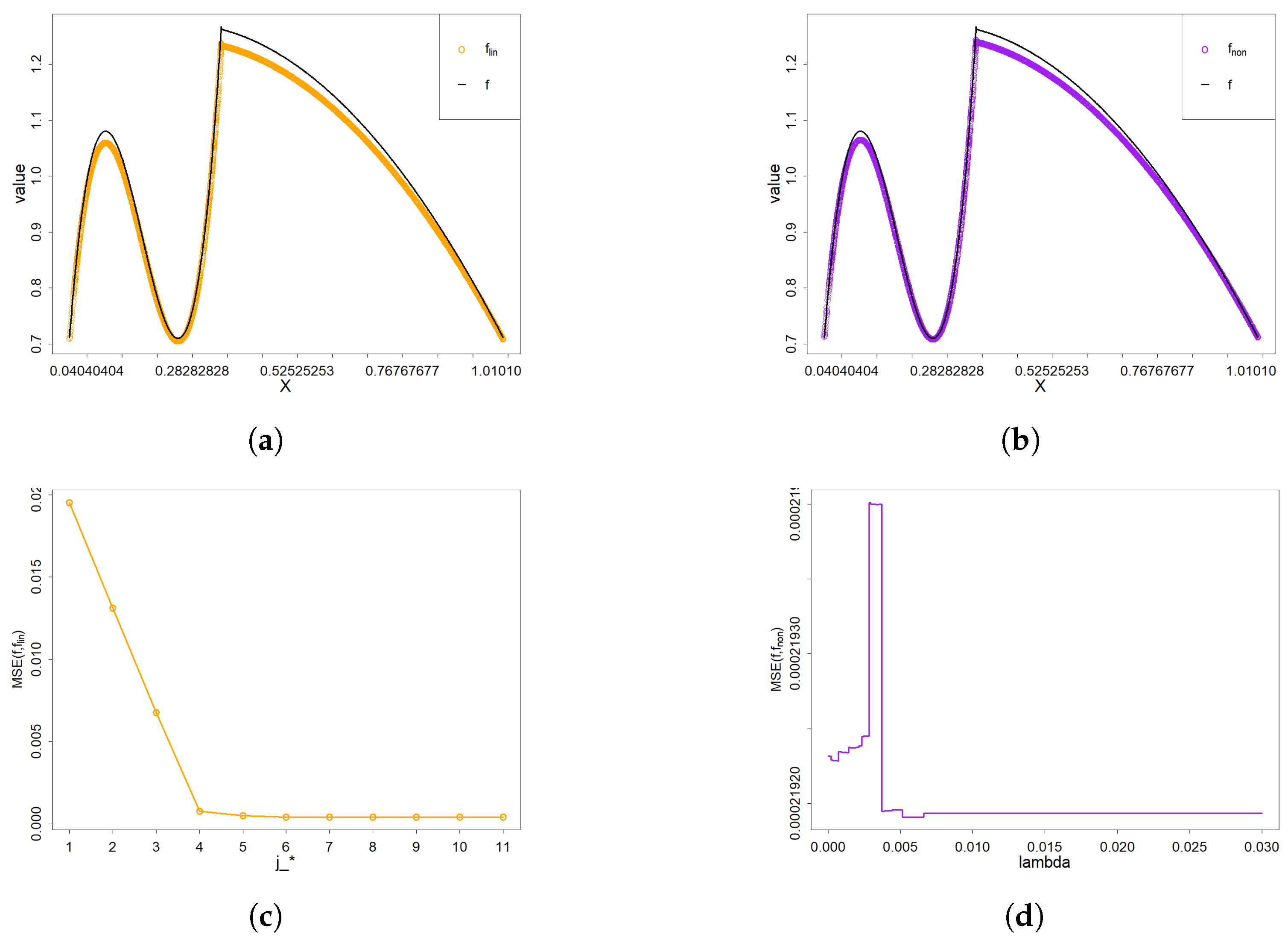
In model (1), we set the unknown density to $f_2(x)=10x{(1-4x{\mathbb{I}}_{\{x\le 0.35\}})}^2{\mathbb{I}}_{\{x\le 0.35\}}+(-x^2+0.5x+0.5){\mathbb{I}}_{\{x>0.35\}}+0.71$, $h(x)=0.7+0.5x^2+0.3cos(2x)$ and $x\in [0, 1]$. The performance of both linear and nonlinear wavelet estimators is illustrated in Figure 2a,b, respectively. Based on Figure 2c,d, the optimal scale parameter $j_0=6$ and the optimal threshold parameter $\lambda =0.0051170569$ are obtained. From those results, it is evident that the nonlinear wavelet estimator outperforms the linear estimator, particularly in capturing sharp features.

Example 3. 

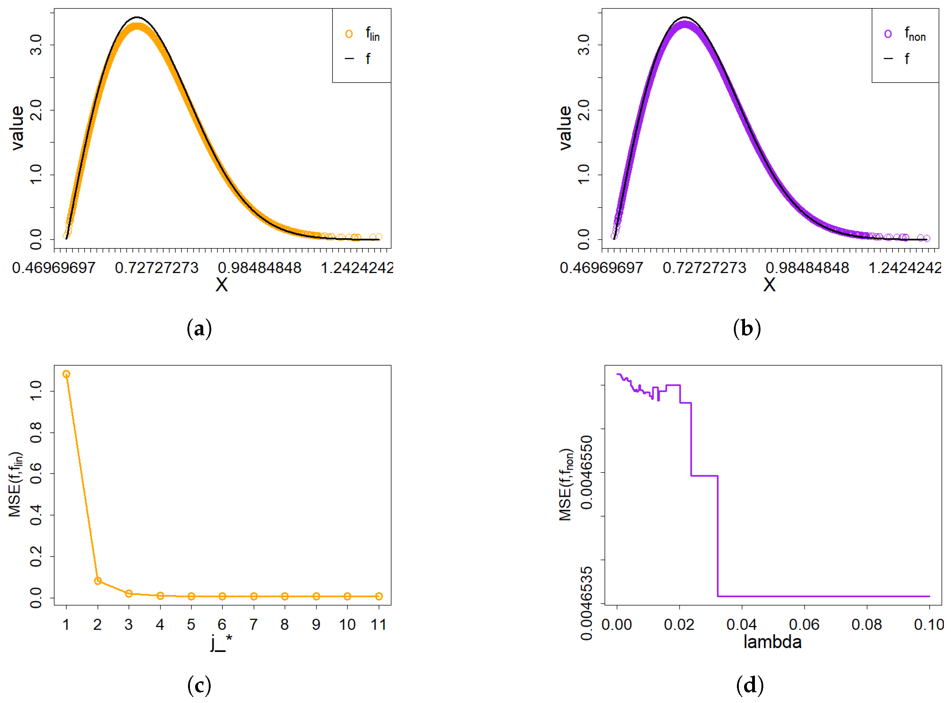
In model (1), we take $f_3(x)=0.81{cos}^{2}x$ on $x\in [-0.5, 1.5]$ and set $h(x)=0.36+0.2x^2+0.1cos(2x)$. The efficacy of the two wavelet estimators in approximating the density function $f(x)$ is evidenced in Figure 3a,b. The corresponding best parameters of two wavelet estimators are presented in Figure 3c,d.

Example 4. 

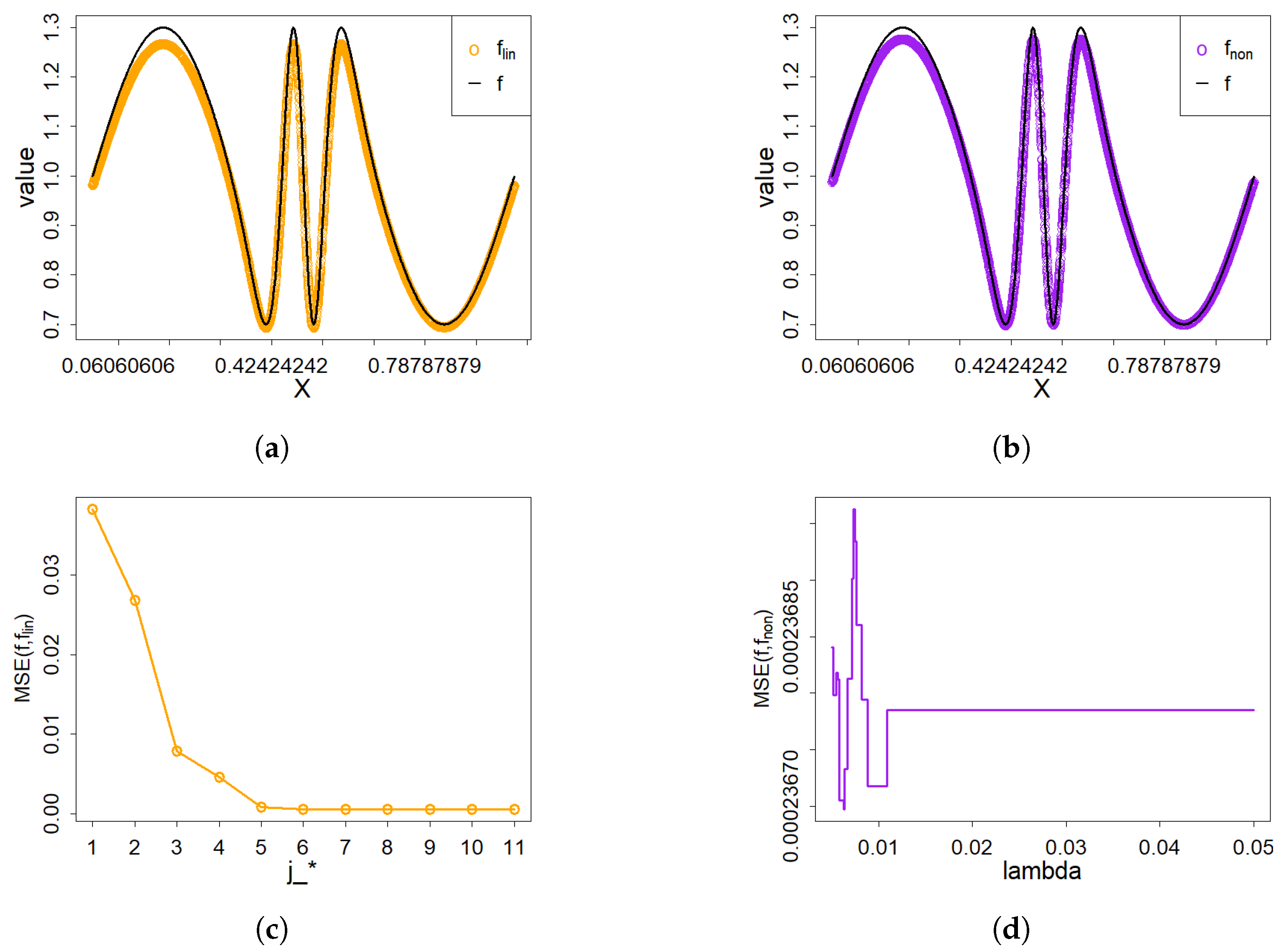
In model (1), the density function is specified as $f_4(x)=2(0.32+0.6x+0.3e^{-100{(x-0.3)}^2}){\mathbb{I}}_{\{x\le 0.5\}}-2(0.28-0.6x-0.3e^{-100{(x-1.3)}^2}){\mathbb{I}}_{\{x>0.5\}}$ with $h(x)=0.43+0.1x^2+0.1cos(2x)$ and $x\in [-1,1]$. The performance of the linear and nonlinear wavelet estimators is illustrated in Figure 4a,b, respectively. Both estimators effectively approximate the density function, but the nonlinear estimator demonstrates superior performance near discontinuities.

Example 5. 

For the experiment, we set the target density to $f_5(x)=(4sin(4\pi x)-sign(x-0.3)-sign(0.72-x))/10+1.1$, $h(x)=0.7+0.5x^2+0.3cos(2x)$ and $x\in [0, 1]$. According to Figure 5c,d, the optimal scale parameter $j_0=5$ and the optimal thresholding parameter $\lambda =0.0929765886$ are obtained. Under these conditions, the density function $f(x)$ can be estimated by the two wavelet estimators shown in Figure 5a,b.

Example 6. 

For the experiment, we select the “Time Shift Sine” as the density function $f_6(x)$ [29]. In addition, $h(x)=0.7+0.5x^2+0.3cos(2x)$ and $x\in [0,1]$. Figure 6c,d show that the optimal scale parameter is $j_0=6$ and the optimal thresholding parameter is $lambda=0.006204013$. From the following results, both wavelet estimators accurately estimate the unknown density.

For both the linear and nonlinear wavelet estimators, the best scale parameter, the optimal thresholding parameter and the values of MSE are shown in

Table 1. Results of the wavelet estimators.

	$f_1$	$f_2$	$f_3$
$j_0$	5	6	9
$\lambda$	0.0321070234	0.0051170569	0.0255852843
$MSE({\widehat{f}}_n^{\mathrm{lin}},f)$	0.0082318890	0.0004092525	0.0004416361
$MSE({\widehat{f}}_n^{\mathrm{non}},f)$	0.0046535810	0.0002191909	0.0002000215
	$f_4$	$f_5$	$f_6$
$j_0$	8	5	6
$\lambda$	0.1056856187	0.0929765886	0.006204013
$MSE({\widehat{f}}_n^{\mathrm{lin}},f)$	0.0024805800	0.0008602093	0.0005513363
$MSE({\widehat{f}}_n^{\mathrm{non}},f)$	0.0012282120	0.0002903662	0.0002366971

. Based on Table 1 and the preceding results, both wavelet estimators effectively approximate the density function, with the nonlinear variant exhibiting superior performance. More importantly, according to the results of Example 2, 4, 5 and 6, both wavelet estimators perform well in cases with discontinuities and spikes.

4. Proof of Main Theorem and Auxiliary Results

In this section, we will give some auxiliary results and the proof of Theorems 1 and 2. It should now be pointed out that this paper does not use symbolic computation software (such as Mathematica, Maple, etc.) for the following theoretical derivations.

4.1. Auxiliary Results

Lemma 2. 

For the model (1), let ${\widehat{a}}_{j,\kappa }$ be defined as (5) and ${\widehat{b}}_{j,\kappa ,\mu }$ given by (7). Then we have

$$\begin{array}{c}\mathrm{E}\left[{\widehat{a}}_{j,\kappa }\right]=a_{j,\kappa },\mathrm{E}\left[{\widehat{b}}_{j,\kappa ,\mu }\right]=b_{j,\kappa ,\mu }.\end{array}$$

Proof. 

Accroding to ${\widehat{a}}_{j,\kappa }=\frac{1}{n}{\displaystyle \sum _{i=1}^n}\frac{1}{1-\theta }{\Phi }_{j,\kappa }(X_i)-{\gamma }_{j,\kappa }$, ${\gamma }_{j,\kappa }={\int }_{\Omega }\frac{\theta }{1-\theta }h(\mathit{x})\Phi (\mathit{x})d\mathit{x}$, we observe that

$$\begin{array}{cc}\hfill \mathrm{E}\left[{\widehat{a}}_{j,\kappa }\right]& =\mathrm{E}\left[\frac{1}{n}\sum _{i=1}^n\frac{1}{1-\theta }{\Phi }_{j,\kappa }(X_i)-{\gamma }_{j,\kappa }\right]\hfill \\ \hfill & =\mathrm{E}\left[\frac{1}{n}\sum _{i=1}^n\frac{1}{1-\theta }{\Phi }_{j,\kappa }(X_i)-{\int }_{\Omega }\frac{\theta }{1-\theta }h(\mathit{x}){\Phi }_{j,\kappa }(\mathit{x})d\mathit{x}\right]\hfill \\ \hfill & =\mathrm{E}\left[\frac{1}{1-\theta }{\Phi }_{j,\kappa }(X_1)\right]-{\int }_{\Omega }\frac{\theta }{1-\theta }h(\mathit{x}){\Phi }_{j,\kappa }(\mathit{x})d\mathit{x}\hfill \\ \hfill & ={\int }_{\Omega }\frac{1}{1-\theta }g(\mathit{x}){\Phi }_{j,\kappa }(\mathit{x})d\mathit{x}-{\int }_{\Omega }\frac{\theta }{1-\theta }h(\mathit{x}){\Phi }_{j,\kappa }(\mathit{x})d\mathit{x}.\hfill \end{array}$$

From the Equation (1), $g(\mathit{x})=\theta h(\mathit{x})+(1-\theta )f(\mathit{x})$ and

$$\begin{array}{cc}\hfill \mathrm{E}\left[{\widehat{a}}_{j,\kappa }\right]& ={\int }_{\Omega }\frac{1}{1-\theta }[\theta h(\mathit{x})+(1-\theta )f(\mathit{x})]{\Phi }_{j,\kappa }(\mathit{x})d\mathit{x}-{\int }_{\Omega }\frac{\theta }{1-\theta }h(\mathit{x}){\Phi }_{j,\kappa }(\mathit{x})d\mathit{x}\hfill \\ \hfill & ={\int }_{\Omega }f(\mathit{x}){\Phi }_{j,\kappa }(\mathit{x})d\mathit{x}\hfill \\ \hfill & ={\langle f,{\Phi }_{j,\kappa }\rangle }_{L_{\Omega }^2}=a_{j,\kappa }.\hfill \end{array}$$

The proof of the second equation is similar to the first one. This concludes the proof of Lemma 2.  □

Lemma 3. 

Consider the model (1) with $\theta \in (0,\delta )$ and $0<\delta <1$. Two unbiased estimators ${\widehat{a}}_{j,\kappa }$ and ${\widehat{b}}_{j,\kappa ,\mu }$ of the wavelet coefficients are proposed by (5) and (7), respectively. Then we have

$$\begin{array}{c}\mathrm{E}\left[{({\widehat{a}}_{j,\kappa }-a_{j,\kappa })}^2\right]\lesssim \frac{1}{n},\mathrm{E}\left[{({\widehat{b}}_{j,\kappa ,\mu }-b_{j,\kappa ,\mu })}^2\right]\lesssim \frac{1}{n}.\end{array}$$

Proof. 

According to Lemma 2 and the definition of ${\gamma }_{j,\kappa }$, one has $\mathbf{var}\left[{\widehat{a}}_{j,\kappa }\right]=\mathrm{E}\left[{({\widehat{a}}_{j,\kappa }-\mathrm{E}\left[{\widehat{a}}_{j,\kappa }\right])}^2\right]$,

$$\begin{array}{cc}\hfill \mathrm{E}\left[{({\widehat{a}}_{j,\kappa }-a_{j,\kappa })}^2\right]& =\mathbf{var}\left[\frac{1}{n}\sum _{i=1}^n\frac{1}{1-\theta }{\Phi }_{j,\kappa }(X_i)-{\gamma }_{j,\kappa }\right]\hfill \\ \hfill & =\mathbf{var}\left[\frac{1}{n}\sum _{i=1}^n\frac{1}{1-\theta }{\Phi }_{j,\kappa }(X_i)\right]\hfill \\ \hfill & =\frac{1}{n^2}\mathbf{var}\left[\sum _{i=1}^n\frac{1}{1-\theta }{\Phi }_{j,\kappa }(X_i)\right]\hfill \\ \hfill & \le \frac{1}{n}\mathrm{E}\left[\frac{1}{{(1-\theta )}^2}{\Phi }_{j,\kappa }^2(X_1)\right]\hfill \\ \hfill & \lesssim \frac{1}{n}\mathrm{E}\left[{\Phi }_{j,\kappa }^2(X_1)\right].\hfill \end{array}$$

Due to the boundness of $h(\mathit{x})$, $f(\mathit{x})$ and mixture parameter $\theta$, we have

$$\begin{array}{cc}\hfill \mathrm{E}\left[{\Phi }_{j,\kappa }^2(X_1)\right]& ={\int }_{\Omega }g(\mathit{x}){\Phi }_{j,\kappa }^2(\mathit{x})d\mathit{x}\hfill \\ \hfill & ={\int }_{\Omega }[\theta h(\mathit{x})+(1-\theta )f(\mathit{x})]{\Phi }_{j,\kappa }^2(\mathit{x})d\mathit{x}\hfill \\ \hfill & ={\int }_{\Omega }\theta h(\mathit{x}){\Phi }_{j,\kappa }^2(\mathit{x})d\mathit{x}+{\int }_{\Omega }(1-\theta )f(\mathit{x}){\Phi }_{j,\kappa }^2(\mathit{x})d\mathit{x}\hfill \\ \hfill & \lesssim {\int }_{\Omega }{\Phi }_{j,\kappa }^2(\mathit{x})d\mathit{x}=1.\hfill \end{array}$$

Hence, we prove the first equality,

$$\mathrm{E}\left[{({\widehat{a}}_{j,\kappa }-a_{j,\kappa })}^2\right]\lesssim \frac{1}{n}.$$

According to the similar arguments, the second equation can be proved easily. Hence, Lemma 3 is proved.  □

Lemma 4. 

Consider the model (1) with $\theta \in (0,\delta )$ and $0<\delta <1$. The wavelet coefficients estimator ${\widehat{b}}_{j,\kappa ,\mu }$ is given by (7). For $2^{jd}\le \frac{n}{lnn}$, with a constant $\tau >1$ satisfying

$$\begin{array}{c}\mathrm{Pr}(|{\widehat{b}}_{j,\kappa ,\mu }-b_{j,\kappa ,\mu }|\ge \tau r_n)\lesssim n^{-4}.\end{array}$$

Proof. 

In order to prove the above result simply, we take

$$B_i:=\frac{1}{1-\theta }\left({\Psi }_{j,\kappa ,\mu }(X_i)-\mathrm{E}\left[{\Psi }_{j,\kappa ,\mu }(X_i)\right]\right).$$

Using Lemma 2,

$$\begin{array}{cc}\hfill \left|{\widehat{b}}_{j,\kappa ,\mu }-b_{j,\kappa ,\mu }\right|& =|\frac{1}{n}\sum _{i=1}^n\frac{1}{1-\theta }{\Psi }_{j,\kappa ,\mu }(X_i)-{\vartheta }_{j,\kappa ,\mu }-\mathrm{E}\left[{\widehat{b}}_{j,\kappa ,\mu }\right]|\hfill \\ \hfill & =|\frac{1}{n}\sum _{i=1}^n\frac{1}{1-\theta }{\Psi }_{j,\kappa ,\mu }(X_i)-\mathrm{E}\left[\frac{1}{1-\theta }{\Psi }_{j,\kappa ,\mu }(X_i)\right]|\hfill \\ \hfill & =\frac{1}{n}\left|\sum _{i=1}^n\frac{1}{1-\theta }({\Psi }_{j,\kappa ,\mu }(X_i)-\mathrm{E}\left[{\Psi }_{j,\kappa ,\mu }(X_i)\right])\right|\hfill \\ \hfill & =\frac{1}{n}\left|\sum _{i=1}^n{B}_i\right|.\hfill \end{array}$$

Thus, the following can be concluded:

$$\mathrm{Pr}\left\{\right|{\widehat{b}}_{j,\kappa ,\mu }-b_{j,\kappa ,\mu }|\ge \tau r_n\}=\mathrm{Pr}\left\{\frac{1}{n}\left|\sum _{i=1}^n{B}_i\right|\ge \tau r_n\right\}.$$

(8)

Note that $\mathrm{E}\left[B_i\right]=0$. The boundness of $h(\mathit{x})$, $f(\mathit{x})$ and $\theta$ imply that

$$\begin{array}{cc}\hfill |B_i|& =\left|\frac{1}{1-\theta }({\Psi }_{j,\kappa ,\mu }(X_i)-\mathrm{E}\left[{\Psi }_{j,\kappa ,\mu }(X_i)\right])\right|\lesssim |{\Psi }_{j,\kappa ,\mu }(X_i)-\mathrm{E}\left[{\Psi }_{j,\kappa ,\mu }(X_i)\right]|\hfill \\ \hfill & \le \left|{\Psi }_{j,\kappa ,\mu }(X_i)\right|+\left|\mathrm{E}\left[{\Psi }_{j,\kappa ,\mu }(X_i)\right]\right|\hfill \\ \hfill & =|2^{\frac{jd}{2}}{\Psi }_{\mu }(2^j{X}_i-\kappa )|+|{\int }_{\Omega }g(\mathit{x})2^{\frac{jd}{2}}{\Psi }_{\mu }(2^j\mathit{x}-\kappa )d\mathit{x}|\lesssim 2^{\frac{jd}{2}}.\hfill \end{array}$$

This together with $2^{jd}\le \frac{n}{lnn}$ shows that

$$|B_i|\lesssim \sqrt{\frac{n}{lnn}}.$$

(9)

On the other hand, using the properties of variance and wavelet function, we have

$$\begin{array}{cc}\hfill \mathrm{E}\left[B_i^2\right]& =\mathrm{E}\left[\frac{1}{{(1-\theta )}^2}{\left({\Psi }_{j,\kappa ,\mu }(X_i)-\mathrm{E}\left[{\Psi }_{j,\kappa ,\mu }(X_i)\right]\right)}^2\right]\hfill \\ \hfill & \lesssim \mathbf{var}\left[{\Psi }_{j,\kappa ,\mu }(X_i)\right]\le \mathrm{E}\left[{\Psi }_{j,\kappa ,\mu }^2(X_i)\right]\lesssim 1.\hfill \end{array}$$

(10)

Finally, it follows from (9), (10) and Bernstein’s inequality [23] that

$$\begin{array}{cc}\hfill \mathrm{Pr}\left(\frac{1}{n}\left|\sum _{i=1}^n{B}_i\right|\ge \tau r_n\right)& \lesssim exp\left\{-\frac{n{\tau }^2{r}_n^2}{2(1+\tau r_n\sqrt{\frac{n}{lnn}}/3)}\right\}\hfill \\ \hfill & \lesssim exp\left\{-\frac{(lnn){\tau }^2}{2(1+\tau /3)}\right\}\lesssim n^{-\frac{{\tau }^2}{2(1+\tau /3)}}.\hfill \end{array}$$

Then, a sufficiently large $\tau$ can be chosen such that

$$\begin{array}{c}\mathrm{Pr}(|{\widehat{b}}_{j,\kappa ,\mu }-b_{j,\kappa ,\mu }|\ge \tau r_n)\lesssim n^{-\frac{{\tau }^2}{2(1+\tau /3)}}\lesssim n^{-4}.\end{array}$$

The proof of Lemma 4 is completed.  □

4.2. Proof of Main Theorem

Proof of Theorem 1.

According to (2) and (3),

$$\begin{array}{cc}\hfill \mathrm{E}[\parallel {\widehat{f}}_n^{\mathrm{lin}}(\mathit{x})-f(\mathit{x}){\parallel }_2^2]& =\mathrm{E}[\parallel {\widehat{f}}_n^{\mathrm{lin}}(\mathit{x})-{\mathrm{P}}_{V_{j_0}}f(\mathit{x})+{\mathrm{P}}_{V_{j_0}}f(\mathit{x})-f(\mathit{x}){\parallel }_2^2]\hfill \\ \hfill & =\mathrm{E}[\parallel {\widehat{f}}_n^{\mathrm{lin}}(\mathit{x})-{\mathrm{P}}_{V_{j_0}}{f(\mathit{x})\parallel }_2^2]+\parallel {\mathrm{P}}_{V_{j_0}}{f(\mathit{x})-f(\mathit{x})\parallel }_2^2.\hfill \end{array}$$

(11)

For the first part, it can be inferred that

$$\begin{array}{cc}\hfill \mathrm{E}[\parallel {\widehat{f}}_n^{\mathrm{lin}}(\mathit{x})-{\mathrm{P}}_{V_{j_0}}f(\mathit{x}){\parallel }_2^2]& =\mathrm{E}\left[{∥\sum _{\kappa \in {\Lambda }_{j_0}}\left({\widehat{a}}_{j_0,\kappa }-a_{j_0,\kappa }\right){\Phi }_{j_0,\kappa }(\mathit{x})∥}^2\right]\hfill \\ \hfill & =\mathrm{E}\left[{\int }_{\Omega }{\left|\sum _{\kappa \in {\Lambda }_{j_0}}\left({\widehat{a}}_{j_0,\kappa }-a_{j_0,\kappa }\right){\Phi }_{j_0,\kappa }(\mathit{x})\right|}^{2}d\mathit{x}\right]\hfill \\ \hfill & =\mathrm{E}\left[\sum _{\kappa \in {\Lambda }_{j_0}}{\left|{\widehat{a}}_{j_0,\kappa }-a_{j_0,\kappa }\right|}^2\right]\hfill \\ \hfill & =\sum _{\kappa \in {\Lambda }_{j_0}}\mathrm{E}\left[{\left|{\widehat{a}}_{j_0,\kappa }-a_{j_0,\kappa }\right|}^2\right].\hfill \end{array}$$

By Lemma 3, since $\left|{\Lambda }_{j_0}\right|\sim 2^{j_{0}d}$ and $2^{j_0}\sim n^{\frac{1}{2s^{\prime }+d}}$, we have

$$\begin{array}{cc}\hfill \mathrm{E}[\parallel {\widehat{f}}_n^{\mathrm{lin}}(\mathit{x})-{\mathrm{P}}_{V_{j_0}}f(\mathit{x}){\parallel }_2^2]& =\sum _{\kappa \in {\Lambda }_{j_0}}\mathrm{E}\left[{\left|{\widehat{a}}_{j_0,\kappa }-a_{j_0,\kappa }\right|}^2\right]\hfill \\ \hfill & \lesssim \sum _{\kappa \in {\Lambda }_{j_0}}\frac{1}{n}=\frac{2^{j_{0}d}}{n}\sim n^{-\frac{2s^{\prime }}{2s^{\prime }+d}}.\hfill \end{array}$$

(12)

For the second part, when $p\ge 2$, we can get $d{(\frac{1}{p}-\frac{1}{2})}_{+}=0$ and $s^{\prime }=s$. Moreover, Hölder’s inequality implies that

$$\begin{array}{cc}\hfill \parallel {\mathrm{P}}_{V_{j_0}}{f(\mathit{x})-f(\mathit{x})\parallel }_2^2& ={\int }_{\Omega }{|{\mathrm{P}}_{V_{j_0}}f(\mathit{x})-f(\mathit{x})|}^2·1d\mathit{x}\hfill \\ \hfill & \le {\left({\int }_{\Omega }{|{\mathrm{P}}_{V_{j_0}}f(\mathit{x})-f(\mathit{x})|}^{2·\frac{p}{2}}d\mathit{x}\right)}^{\frac{2}{p}}{\left({\int }_{\Omega }{1}^{1^{\frac{p}{p-2}}}d\mathit{x}\right)}^{1-\frac{2}{p}}\hfill \\ \hfill & \lesssim {\left({\int }_{\Omega }{|{\mathrm{P}}_{V_{j_0}}f(\mathit{x})-f(\mathit{x})|}^{p}d\mathit{x}\right)}^{\frac{2}{p}}\hfill \\ \hfill & =\parallel {\mathrm{P}}_{V_{j_0}}{f(\mathit{x})-f(\mathit{x})\parallel }_p^2.\hfill \end{array}$$

Furthermore, using Lemma 1 and $f(\mathit{x})\in B_{p,q}^s(\Omega )$, we can get

$$\begin{array}{c}\parallel {\mathrm{P}}_{V_{j_0}}{f(\mathit{x})-f(\mathit{x})\parallel }_2^2\lesssim {\parallel {\mathrm{P}}_{V_{j_0}}f(\mathit{x})-f(\mathit{x})\parallel }_p^2\lesssim 2^{-j_{0}s}\sim n^{-\frac{2s}{2s+d}}.\end{array}$$

(13)

When $1\le p<2$ and $s>\frac{d}{p}$, we know that $s^{\prime }=s-d(\frac{1}{p}-\frac{1}{2})$ and $B_{p,q}^s(\Omega )\subseteq B_{2,+\infty }^{s^{\prime }}(\Omega )$. In addition, the following conclusion is true,

$$\begin{array}{c}\hfill \parallel {\mathrm{P}}_{V_{j_0}}{f(\mathit{x})-f(\mathit{x})\parallel }_2^2\lesssim \sum _{j=j_0}^{\infty }{2}^{-2j{s}^{\prime }}\sim 2^{-2j_0{s}^{\prime }}\sim n^{-\frac{2s^{\prime }}{2s^{\prime }+d}}.\end{array}$$

(14)

Hence, for $1\le p<\infty$, the results (13) and (14) show that

$$\begin{array}{c}\parallel {\mathrm{P}}_{V_{j_0}}{f(\mathit{x})-f(\mathit{x})\parallel }_2^2\lesssim n^{-\frac{2s^{\prime }}{2s^{\prime }+d}}.\end{array}$$

(15)

Finally, together with (11), (12) and (15), we prove that

$$\begin{array}{c}\mathrm{E}[\parallel {\widehat{f}}_n^{\mathrm{lin}}(\mathit{x})-f(\mathit{x}){\parallel }_2^2]\lesssim n^{-\frac{2s^{\prime }}{2s^{\prime }+d}}.\end{array}$$

□

Proof of Theorem 2.

According to the definitions of linear estimator, nonlinear estimator and projection operator, we have

$$\begin{array}{cc}\hfill {\widehat{f}}_n^{\mathrm{non}}(\mathit{x})-f(\mathit{x})& =({\widehat{f}}_n^{\mathrm{lin}}(\mathit{x})-{\mathrm{P}}_{V_{j_0}}f(\mathit{x}))-(f(\mathit{x})-{\mathrm{P}}_{V_{j_2+1}}f(\mathit{x}))\hfill \\ \hfill & +\sum _{j=j_0}^{{\mathrm{j}}_1}\sum _{\mu =1}^{2^d-1}\sum _{\kappa \in {\Lambda }_j}({\widehat{b}}_{j,\kappa ,\mu }{\mathbb{I}}_{\{|{\widehat{b}}_{j,\kappa ,\mu }|\ge \tau r_n\}}-b_{j,\kappa ,\mu }){\Psi }_{j,\kappa ,\mu }(\mathit{x}).\hfill \end{array}$$

Hence,

$$\begin{array}{c}\hfill \mathrm{E}[\parallel {\widehat{f}}_n^{\mathrm{non}}(\mathit{x})-f(\mathit{x}){\parallel }_2^2]\lesssim T_1+T_2+D.\end{array}$$

(16)

In this inequality,

$$\begin{array}{c}{T}_1:=\mathrm{E}\left[{∥{\widehat{f}}_n^{\mathrm{lin}}(\mathit{x})-{\mathrm{P}}_{V_{j_0}}f(\mathit{x})∥}_2^2\right],\\ T_2:={∥f(\mathit{x})-{\mathrm{P}}_{V_{j_2+1}}f(\mathit{x})∥}_2^2,\\ D:=\mathrm{E}\left[{∥\sum _{j=j_0}^{j_2}\sum _{\mu =1}^{2^d-1}\sum _{\kappa \in {\Lambda }_j}\left({\widehat{b}}_{j,\kappa ,\mu }{\mathbb{I}}_{\left\{|{\widehat{b}}_{j,\kappa ,\mu }|\ge \tau r_n\right\}}-b_{j,\kappa ,\mu }\right){\Psi }_{j,\kappa ,\mu }(\mathit{x})∥}_2^2\right].\end{array}$$

For $T_1$. According to Lemma 3, (12) and $2^{j_0}\sim n^{\frac{1}{2\omega +d}}(\omega >s)$,

$$\begin{array}{cc}\hfill T_1& =\mathrm{E}\left[{∥{\widehat{f}}_n^{\mathrm{lin}}(\mathit{x})-{\mathrm{P}}_{V_{j_0}}f(\mathit{x})∥}_2^2\right]\hfill \\ \hfill & =\sum _{\kappa \in {\Lambda }_{j_0}}\mathrm{E}\left[{\left|{\widehat{a}}_{j_0,\kappa }-a_{j_0,\kappa }\right|}^2\right]\lesssim \sum _{\kappa \in {\Lambda }_{j_0}}\frac{1}{n}\hfill \\ \hfill & \lesssim \frac{2^{j_{0}d}}{n}\sim n^{-\frac{2\omega }{2\omega +d}}\le n^{-\frac{2s}{2s+d}}.\hfill \end{array}$$

(17)

For $T_2$. Consistent with the reasoning in (15), it follows that

$$\begin{array}{c}{T}_2\lesssim (lnn)n^{-\frac{2s}{2s+d}},\end{array}$$

(18)

with the condition $2^{j_2}\sim {(\frac{n}{lnn})}^{\frac{1}{d}}$.

The following work is to prove

$$\begin{array}{c}D=\mathrm{E}\left[{∥\sum _{j=j_0}^{j_2}\sum _{\mu =1}^{2^d-1}\sum _{\kappa \in {\Lambda }_j}\left({\widehat{b}}_{j,\kappa ,\mu }{\mathbb{I}}_{\left\{|{\widehat{b}}_{j,\kappa ,\mu }|\ge \tau r_n\right\}}-b_{j,\kappa ,\mu }\right){\Psi }_{j,\kappa ,\mu }(\mathit{x})∥}_2^2\right]\lesssim (lnn)n^{-\frac{2s}{2s+d}}.\end{array}$$

According to the properties of wavelet function, we have

$$\begin{array}{c}D=\sum _{j=j_0}^{j_2}\sum _{\mu =1}^{2^d-1}\sum _{\kappa \in {\Lambda }_j}\mathrm{E}\left[{\left|{\widehat{b}}_{j,\kappa ,\mu }{\mathbb{I}}_{\{|{\widehat{b}}_{j,\kappa ,\mu }|\ge \tau r_n\}}-b_{j,\kappa ,\mu }\right|}^2\right].\end{array}$$

Note that the following conclusion is true:

$$\begin{array}{cc}\hfill {\left|{\widehat{b}}_{j,\kappa ,\mu }{\mathbb{I}}_{\{|{\widehat{b}}_{j,\kappa ,\mu }|\ge \tau r_n\}}-b_{j,\kappa ,\mu }\right|}^2& \lesssim {\left|{\widehat{b}}_{j,\kappa ,\mu }-b_{j,\kappa ,\mu }\right|}^2{\mathbb{I}}_{\{|{\widehat{b}}_{j,\kappa ,\mu }-b_{j,\kappa ,\mu }|>\frac{\tau r_n}{2}\}}\hfill \\ \hfill & +{\left|{\widehat{b}}_{j,\kappa ,\mu }-b_{j,\kappa ,\mu }\right|}^2{\mathbb{I}}_{\{|b_{j,\kappa ,\mu }|>\frac{\tau r_n}{2}\}}+{\left|b_{j,\kappa ,\mu }\right|}^2{\mathbb{I}}_{\{b_{j,\kappa ,\mu }|\le 2\tau r_n\}}.\hfill \end{array}$$

Then, we have

$$\begin{array}{c}D=\sum _{j=j_0}^{j_2}\sum _{\mu =1}^{2^d-1}\sum _{\kappa \in {\Lambda }_j}\mathrm{E}\left[{\left|{\widehat{b}}_{j,\kappa ,\mu }{\mathbb{I}}_{\{|{\widehat{b}}_{j,\kappa ,\mu }|\ge \tau r_n\}}-b_{j,\kappa ,\mu }\right|}^2\right]\lesssim D_1+D_2+D_3,\end{array}$$

(19)

$$\begin{array}{c}{D}_1=\sum _{j=j_0}^{j_2}\sum _{\mu =1}^{2^d-1}\sum _{\kappa \in {\Lambda }_j}\mathrm{E}\left[{\left|{\widehat{b}}_{j,\kappa ,\mu }-b_{j,\kappa ,\mu }\right|}^2{\mathbb{I}}_{\{|{\widehat{b}}_{j,\kappa ,\mu }-b_{j,\kappa ,\mu }|>\frac{\tau r_n}{2}\}}\right],\\ D_2=\sum _{j=j_0}^{j_2}\sum _{\mu =1}^{2^d-1}\sum _{\kappa \in {\Lambda }_j}\mathrm{E}\left[{\left|{\widehat{b}}_{j,\kappa ,\mu }-b_{j,\kappa ,\mu }\right|}^2{\mathbb{I}}_{\{|b_{j,\kappa ,\mu }|\ge \frac{\tau r_n}{2}\}}\right],\\ D_3=\sum _{j=j_0}^{j_2}\sum _{\mu =1}^{2^d-1}\sum _{\kappa \in {\Lambda }_j}{\left|b_{j,\kappa ,\mu }\right|}^2{\mathbb{I}}_{\{|b_{j,\kappa ,\mu }|\le 2\tau r_n\}}.\end{array}$$

For $D_1$. Applying Hölder inequality,

$$\begin{array}{cc}\hfill \mathrm{E}\left[{\left|{\widehat{b}}_{j,\kappa ,\mu }-b_{j,\kappa ,\mu }\right|}^2{\mathbb{I}}_{\{|{\widehat{b}}_{j,\kappa ,\mu }-b_{j,\kappa ,\mu }|>\frac{\tau r_n}{2}\}}\right]& \le {\left(\mathrm{E}[|{\widehat{b}}_{j,\kappa ,\mu }-b_{j,\kappa ,\mu }{|}^4]\right)}^{\frac{1}{2}}{\left(\mathrm{E}\left[{\mathbb{I}}_{\{|{\widehat{b}}_{j,\kappa ,\mu }-b_{j,\kappa ,\mu }|>\frac{\tau r_n}{2}\}}\right]\right)}^{\frac{1}{2}}\hfill \\ \hfill & \le {\left(\mathrm{E}[|{\widehat{b}}_{j,\kappa ,\mu }-b_{j,\kappa ,\mu }{|}^4]\right)}^{\frac{1}{2}}{\left(\mathrm{Pr}\left(|{\widehat{b}}_{j,\kappa ,\mu }-b_{j,\kappa ,\mu }|\ge \frac{\tau r_n}{2}\right)\right)}^{\frac{1}{2}}.\hfill \end{array}$$

According to Lemmas 3 and 4,

$$\begin{array}{cc}\hfill \mathrm{E}\left[{\left|{\widehat{b}}_{j,\kappa ,\mu }-b_{j,\kappa ,\mu }\right|}^2{\mathbb{I}}_{\{|{\widehat{b}}_{j,\kappa ,\mu }-b_{j,\kappa ,\mu }|>\frac{\tau r_n}{2}\}}\right]& \le {\left(\mathrm{E}\left[{\left|{\widehat{b}}_{j,\kappa ,\mu }-b_{j,\kappa ,\mu }\right|}^2{({\widehat{b}}_{j,\kappa ,\mu }-b_{j,\kappa ,\mu })}^2\right]\right)}^{\frac{1}{2}}.\frac{1}{n^2}\hfill \\ \hfill & \lesssim {\left(\frac{n}{lnn}\mathrm{E}\left[{({\widehat{b}}_{j,\kappa ,\mu }-b_{j,\kappa ,\mu })}^2\right]\right)}^{\frac{1}{2}}.\frac{1}{n^2}\hfill \\ \hfill & \lesssim \frac{1}{n^2\sqrt{lnn}}.\hfill \end{array}$$

Then, $D_1\lesssim \sum _{j=j_0}^{j_2}\frac{2^{jd}}{n^2\sqrt{lnn}}\lesssim \frac{2^{j_{2}d}}{n^2\sqrt{lnn}}\lesssim \frac{1}{n{(lnn)}^{\frac{3}{2}}}\le \frac{1}{n}\le n^{-\frac{2s}{2s+d}}$. Hence,

$$\begin{array}{c}{D}_1\lesssim n^{-\frac{2s}{2s+d}}.\end{array}$$

(20)

For $D_2$. We define $2^{j_1}\sim n^{\frac{1}{2s+d}}$. Then $2^{j_0}\sim n^{\frac{1}{2\omega +d}}(\omega >s)\le 2^{j_1}\sim n^{\frac{1}{2s+d}}\le 2^{j_2}\sim {\left(\frac{n}{lnn}\right)}^{\frac{1}{d}}$. Moreover, we can rewrite $D_2$ as

$$\begin{array}{cc}\hfill D_2& :=\left(\sum _{j=j_0}^{j_1}+\sum _{j=j_1+1}^{j_2}\right)\left\{\sum _{\mu =1}^{2^d-1}\sum _{\kappa \in {\Lambda }_j}\mathrm{E}\left[{\left|{\widehat{b}}_{j,\kappa ,\mu }-b_{j,\kappa ,\mu }\right|}^2{\mathbb{I}}_{\{|b_{j,\kappa ,\mu }|\ge \frac{\tau r_n}{2}\}}\right]\right\}\hfill \\ \hfill & :=D_{21}+D_{22}.\hfill \end{array}$$

(21)

Using Lemma 3,

$$\begin{array}{cc}\hfill D_{21}& =\sum _{j=j_0}^{j_1}\sum _{\mu =1}^{2^d-1}\sum _{\kappa \in {\Lambda }_j}\mathrm{E}\left[{\left|{\widehat{b}}_{j,\kappa ,\mu }-b_{j,\kappa ,\mu }\right|}^2{\mathbb{I}}_{\{|b_{j,\kappa ,\mu }|\ge \frac{\tau r_n}{2}\}}\right]\hfill \\ \hfill & \lesssim \sum _{j=j_0}^{j_1}\sum _{\mu =1}^{2^d-1}\sum _{\kappa \in {\Lambda }_j}\frac{1}{n}\lesssim \sum _{j=j_0}^{j_1}\frac{2^{jd}}{n}\lesssim \frac{2^{j_{1}d}}{n}\sim n^{-\frac{2s}{2s+d}}.\hfill \end{array}$$

(22)

For $D_{22}$, note that

$$\begin{array}{cc}\hfill D_{22}& :=\sum _{j=j_1+1}^{j_2}\sum _{\mu =1}^{2^d-1}\sum _{\kappa \in {\Lambda }_j}\mathrm{E}\left[{\left|{\widehat{b}}_{j,\kappa ,\mu }-b_{j,\kappa ,\mu }\right|}^2{\mathbb{I}}_{\{|b_{j,\kappa ,\mu }|\ge \frac{\tau r_n}{2}\}}\right]\hfill \\ \hfill & \lesssim \sum _{j=j_1+1}^{j_1}\sum _{\mu =1}^{2^d-1}\sum _{\kappa \in {\Lambda }_j}\frac{1}{n}{\mathbb{I}}_{\{|b_{j,\kappa ,\mu }|\ge \frac{\tau r_n}{2}\}}.\hfill \end{array}$$

For $p\ge 2$, according to $f\in B_{p,q}^s(\Omega )$, $r_n=\sqrt{\frac{lnn}{n}}$ and Hölder inequality,

$$\begin{array}{cc}\hfill D_{22}& \lesssim \sum _{j=j_1+1}^{j_1}\sum _{\mu =1}^{2^d-1}\sum _{\kappa \in {\Lambda }_j}\frac{1}{n}{\left(\frac{|b_{j,\kappa ,\mu }|}{\tau r_n/2}\right)}^2\lesssim \sum _{j=j_1+1}^{j_2}\sum _{\mu =1}^{2^d-1}\sum _{\kappa \in {\Lambda }_j}{|b_{j,\kappa ,\mu }|}^2\hfill \\ \hfill & =\sum _{j=j_1+1}^{j_2}\parallel b_{j,\kappa ,\mu }{\parallel }_2^2\le \sum _{j=j_1+1}^{j_2}{2}^{jd(1-\frac{2}{p})}{\parallel b_{j,\kappa ,\mu }\parallel }_p^2\hfill \\ \hfill & \lesssim \sum _{j=j_1+1}^{j_2}{2}^{-2js}\lesssim 2^{-2j_{1}s}\sim n^{-\frac{2s}{2s+d}}.\hfill \end{array}$$

(23)

On the other hand, in the case of $1\le p<2$, by Lemma 1 and the definition of $2^{j_1}$,

$$\begin{array}{cc}\hfill D_{22}& \lesssim \sum _{j=j_1+1}^{j_2}\sum _{\mu =1}^{2^d-1}\sum _{\kappa \in {\Lambda }_j}\frac{1}{n}{\mathbb{I}}_{\{|b_{j,\kappa ,\mu }|\ge \frac{\tau r_n}{2}\}}\hfill \\ \hfill & \le \sum _{j=j_1+1}^{j_2}\sum _{\mu =1}^{2^d-1}\sum _{\kappa \in {\Lambda }_j}\frac{1}{n}{\left(\frac{|b_{j,\kappa ,\mu }|}{\tau r_n/2}\right)}^p\lesssim (lnn)n^{\frac{p}{2}-1}\sum _{j=j_1+1}^{j_2}{\parallel b_{j,\kappa ,\mu }\parallel }_p^p\hfill \\ \hfill & \lesssim (lnn)n^{\frac{p}{2}-1}\sum _{j=j_1+1}^{j_2}{2}^{-j(s+\frac{d}{2}-\frac{d}{p})p}\lesssim (lnn)n^{\frac{p}{2}-1}{2}^{-j_1(s+\frac{d}{2}-\frac{d}{p})p}\hfill \\ \hfill & \sim (lnn)n^{-\frac{2s}{2s+d}}.\hfill \end{array}$$

(24)

This with (21)–(23) shows that

$$\begin{array}{c}{D}_2\lesssim (lnn)n^{-\frac{2s}{2s+d}}.\end{array}$$

(25)

For $D_3$, it could be written as

$$\begin{array}{cc}\hfill D_3& =\left(\sum _{j=j_0}^{j_1}+\sum _{j=j_1+1}^{j_2}\right)\sum _{\mu =1}^{2^d-1}\sum _{\kappa \in {\Lambda }_j}{\left|b_{j,\kappa ,\mu }\right|}^2{\mathbb{I}}_{\{|b_{j,\kappa ,\mu }|\le 2\tau r_n\}}\hfill \\ \hfill & :=D_{31}+D_{32}.\hfill \end{array}$$

(26)

For the upper bound of $D_{31}$, it is easily to get that

$$\begin{array}{cc}\hfill D_{31}& =\sum _{j=j_0}^{j_1}\sum _{\mu =1}^{2^d-1}\sum _{\kappa \in {\Lambda }_j}{\left|b_{j,\kappa ,\mu }\right|}^2{\mathbb{I}}_{\{|b_{j,\kappa ,\mu }|\le 2\tau r_n\}}\hfill \\ \hfill & \le \sum _{j=j_0}^{j_1}\sum _{\mu =1}^{2^d-1}\sum _{\kappa \in {\Lambda }_j}{|2\tau r_n|}^2\lesssim \sum _{j=j_0}^{j_1}\frac{lnn}{n}{2}^{jd}\hfill \\ \hfill & \lesssim \frac{lnn}{n}{2}^{j_{1}d}\lesssim (lnn)n^{-\frac{2s}{2s+d}}.\hfill \end{array}$$

(27)

For the upper bound for $D_{32}$, when $p\ge 2$, using Lemma 1 and Hölder’s inequality,

$$\begin{array}{cc}\hfill D_{32}& =\sum _{j=j_1+1}^{j_2}\sum _{\mu =1}^{2^d-1}\sum _{\kappa \in {\Lambda }_j}{\left|b_{j,\kappa ,\mu }\right|}^2{\mathbb{I}}_{\{|b_{j,\kappa ,\mu }|\le 2\tau r_n\}}\hfill \\ \hfill & \lesssim \sum _{j=j_1+1}^{j_2}\sum _{\mu =1}^{2^d-1}\sum _{\kappa \in {\Lambda }_j}{\left|b_{j,\kappa ,\mu }\right|}^2\lesssim \sum _{j=j_1+1}^{j_2}{2}^{jd(1-\frac{p}{2})}{\parallel b_{j,\kappa ,\mu }\parallel }_p^2\hfill \\ \hfill & \lesssim \sum _{j=j_1+1}^{j_2}{2}^{-2js}\lesssim 2^{-2j_{1}s}\sim n^{-\frac{2s}{2s+d}}.\hfill \end{array}$$

(28)

For $1\le p<2$, have ${\left|b_{j,\kappa ,\mu }\right|}^2{\mathbb{I}}_{\{|b_{j,\kappa ,\mu }|\le 2\tau r_n\}}\le |b_{j,\kappa ,\mu }{|}^p{|2\tau r_n|}^{2-p}$. Furthermore,

$$\begin{array}{cc}\hfill D_{32}& =\sum _{j=j_1+1}^{j_2}\sum _{\mu =1}^{2^d-1}\sum _{\kappa \in {\Lambda }_j}{\left|b_{j,\kappa ,\mu }\right|}^2{\mathbb{I}}_{\{|b_{j,\kappa ,\mu }|\le 2\tau r_n\}}\hfill \\ \hfill & \lesssim \sum _{j=j_1+1}^{j_2}\sum _{\mu =1}^{2^d-1}\sum _{\kappa \in {\Lambda }_j}|b_{j,\kappa ,\mu }{|}^p|2\tau r_n{|}^{2-p}\lesssim \sum _{j=j_1+1}^{j_2}{\parallel b_{j,\kappa ,\mu }\parallel }_p^p{\left(\frac{lnn}{n}\right)}^{\frac{2-p}{2}}\hfill \\ \hfill & \lesssim {\left(\frac{lnn}{n}\right)}^{\frac{2-p}{2}}\sum _{j=j_1+1}^{j_2}{2}^{-j(s+\frac{d}{2}-\frac{d}{p})p}\lesssim {\left(\frac{lnn}{n}\right)}^{\frac{2-p}{2}}{2}^{-j_1(s+\frac{d}{2}-\frac{d}{p})p}\hfill \\ \hfill & \lesssim (lnn)n^{-\frac{2s}{2s+d}}.\hfill \end{array}$$

(29)

Then, according to (26)–(29),

$$\begin{array}{c}{D}_3\lesssim (lnn)n^{-\frac{2s}{2s+d}}.\end{array}$$

(30)

Due to (19), (20), (25) and (30), we can prove that

$$\begin{array}{c}D\lesssim (lnn)n^{-\frac{2s}{2s+d}}.\end{array}$$

Together with (16)–(18), this yields

$$\begin{array}{c}\mathrm{E}[\parallel {\widehat{f}}_n^{\mathrm{non}}(\mathit{x})-f(\mathit{x}){\parallel }_2^2]\lesssim (lnn)n^{-\frac{2s}{2s+d}}.\end{array}$$

□

5. Conclusions

This paper systematically investigates the application of wavelet methods in density estimation under nonparametric mixture models. Under mild regularity conditions, two estimators are constructed: a linear estimator and a nonlinear adaptive estimator. Meanwhile, we conduct theoretical analysis to derive the convergence rates of these estimators under the $L^2$-risk criterion. Results demonstrate that both estimation methods achieve optimal convergence rates in nonparametric density estimation, thereby confirming their statistical efficiency. Furthermore, numerical experiments validate that the practical performance of the proposed methods aligns with theoretical conclusions, indicating their robust statistical efficiency.

References

1. Huber, P.J. A robust version of the probability ratio test. Ann. Math. Stat. 1965, 36, 1753–1758. [Google Scholar] [CrossRef]
2. McLachlan, G.; Peel, D. Finite Mixture Models; Wiley: New York, NY, USA, 2000. [Google Scholar]
3. Allison, D.B.; Gadbury, G.L.; Heo, M.; Fernández, J.R.; Lee, C.K.; Prolla, T.A.; Weindruch, R. A mixture model approach for the analysis of microarray gene expression data. Comput. Stat. Data Anal. 2002, 39, 1–20. [Google Scholar] [CrossRef]
4. Aubert, J.; Bar-Hen, A.; Daudin, J.J.; Robin, S. Determination of the differentially expressed genes in microarray experiments using local FDR. BMC Bioinform. 2004, 5, 125. [Google Scholar] [CrossRef]
5. Liao, J.G.; Lin, Y.; Selvanayagam, Z.E.; Shih, W.J. A mixture model for estimating the local false discovery rate in DNA microarray analysis. Bioinformatics 2004, 20, 2694–2701. [Google Scholar] [CrossRef] [PubMed]
6. Shu, H.; Nan, B.; Koeppe, R. Multiple testing for neuroimaging via hidden markov random field. Biometrics 2015, 71, 741–750. [Google Scholar] [CrossRef] [PubMed]
7. Efron, B. Large-scale simultaneous hypothesis testing. J. Am. Stat. Assoc. 2004, 99, 96–104. [Google Scholar] [CrossRef]
8. McLachlan, G.J.; Bean, R.W.; Jones, L.B.T. A simple implementation of a normal mixture approach to differential gene expression in multiclass microarrays. Bioinformatics 2006, 22, 1608–1615. [Google Scholar] [CrossRef]
9. Efron, B.; Tibshirani, R.; Storey, J.D.; Tusher, V. Empirical bayes analysis of a microarray experiment. J. Am. Stat. Assoc. 2001, 96, 1151–1160. [Google Scholar] [CrossRef]
10. Olkin, I.; Spiegelman, C.H. A semiparametric approach to density estimation. J. Am. Stat. Assoc. 1987, 82, 858–865. [Google Scholar] [CrossRef]
11. Priebe, C.E.; Marchette, D.J. Alternating kernel and mixture density estimates. Comput. Stat. Data Anal. 2000, 35, 43–65. [Google Scholar] [CrossRef]
12. James, L.F.; Priebe, C.E.; Marchette, D.J. Consistent estimation of mixture complexity. Ann. Stat. 2001, 29, 1281–1296. [Google Scholar] [CrossRef]
13. Robin, S.; Bar-Hen, A.; Daudin, J.J.; Pierre, L. A semi-parametric approach for mixture models: Application to local false discovery rate estimation. Comput. Stat. Data Anal. 2007, 51, 5483–5493. [Google Scholar] [CrossRef]
14. Nguyen, V.H.; Matias, C. Nonparametric estimation of the density of the alternative hypothesis in a multiple testing setup. Application to local false discovery rate estimation. ESAIM Probab. Stat. 2014, 18, 584–612. [Google Scholar] [CrossRef]
15. Patra, R.K.; Sen, B. Estimation of a two-component mixture model with applications to multiple testing. J. R. Stat. Soc. Ser. B Stat. Methodol. 2016, 78, 869–893. [Google Scholar] [CrossRef]
16. Deb, N.; Saha, S.; Guntuboyina, A.; Sen, B. Two-component mixture model in the presence of covariates. J. Am. Stat. Assoc. 2022, 117, 1820–1834. [Google Scholar] [CrossRef]
17. Chesneau, C.; Doosti, H.; Stone, L. Adaptive wavelet estimation of a function from an m-dependent process with possibly unbounded m. Commun. Stat.-Theory Methods 2018, 48, 1123–1135. [Google Scholar] [CrossRef]
18. Amato, U.; Antoniadis, A.; Feis, I.D.; Gijbels, I. Wavelet-based robust estimation and variable selection in nonparametric additive models. Stat. Comput. 2022, 32, 11. [Google Scholar] [CrossRef]
19. Niles-Weed, J.; Berthet, Q. Minimax estimation of smooth densities in wasserstein distance. Ann. Stat. 2022, 50, 1519–1540. [Google Scholar] [CrossRef]
20. Shirazi, E.; Doosti, H. Evaluation of threshold selection methods for adaptive wavelet quantile density estimation in the presence of bias. Commun. Stat.-Simul. Comput. 2024, 53, 6633–6646. [Google Scholar] [CrossRef]
21. Benhaddou, R.; Liu, Q. Wavelet estimation for the nonparametric additive model in random design and long-memory dependent errors. J. Nonparametric Stat. 2024, 36, 1088–1113. [Google Scholar] [CrossRef]
22. Rademacher, D.; Krebs, J.; Sachs, R.V. Statistical inference for wavelet curve estimators of symmetric positive definite matrices. J. Stat. Plan. Inference 2024, 231, 106140. [Google Scholar] [CrossRef]
23. Härdle, W.; Kerkyacharian, G.; Picard, D.; Tsybakov, A. Wavelets, Approximation and Statistical Applications; Springer: New York, NY, USA, 1997. [Google Scholar]
24. Daubechies, I. Ten Lectures on Wavelets; SIAM: Philadelphia, PA, USA, 1992. [Google Scholar]
25. Boggess, A.; Narcowich, F.J. A First Course in Wavelets with Fourier Analysis; Wiley and Sons: Toronto, ON, Canada, 2009. [Google Scholar]
26. Donoho, D.L.; Johnstone, M.I.; Kerkyacharian, G.; Picard, D. Density estimation by wavelet thresholding. Ann. Stat. 1996, 24, 508–539. [Google Scholar] [CrossRef]
27. Juditsky, A.; Lambert-Lacroix, S. On minimax density estimation on R. Bernoulli 2004, 10, 187–220. [Google Scholar] [CrossRef]
28. Reynaud-Bouret, P.; Rivoirard, V.; Tuleau-Malot, C. Adaptive density estimation: A curse of support. J. Stat. Plan. Inference 2011, 141, 115–139. [Google Scholar] [CrossRef]
29. Chesneau, C.; Kolei, S.E.; Kou, J.K.; Navarro, F. Nonparametric estimation in a regression model with additive and multiplicative noise. J. Comput. Appl. Math. 2020, 380, 112971. [Google Scholar] [CrossRef]
Figure 1. Estimations of two wavelet estimators with density function f ( x ) = f 1 ( x ) . (a) Linear wavelet estimator result f ^ n lin ( x ) ; (b) nonlinear wavelet estimator result f ^ n non ( x ) ; (c) M S E ( f ^ n lin , f ) with different scale parameter j 0 ; (d) M S E ( f ^ n non , f ) with different thresholding parameter λ .
Axioms 14 00741 g001
Figure 2. Estimations of two wavelet estimators with density function f ( x ) = f 2 ( x ) . (a) Linear wavelet estimator result f ^ n lin ( x ) ; (b) nonlinear wavelet estimator result f ^ n non ( x ) ; (c) M S E ( f ^ n lin , f ) under different scale parameters j 0 ; (d) M S E ( f ^ n non , f ) under different threshold parameters λ .
Axioms 14 00741 g002
Figure 3. Estimations of two wavelet estimators with density function f ( x ) = f 3 ( x ) . (a) Linear wavelet estimator result f ^ n lin ( x ) ; (b) nonlinear wavelet estimator result f ^ n non ( x ) ; (c) M S E ( f ^ n lin , f ) with different scale parameter j 0 ; (d) M S E ( f ^ n non , f ) with different thresholding parameter λ .
Axioms 14 00741 g003
Figure 4. Estimations of two wavelet estimators with density function f ( x ) = f 4 ( x ) . (a) Linear wavelet estimator result f ^ n lin ( x ) ; (b) nonlinear wavelet estimator result f ^ n non ( x ) ; (c) M S E ( f ^ n lin , f ) under different scale parameters j 0 ; (d) M S E ( f ^ n non , f ) under different threshold parameters λ .
Axioms 14 00741 g004
Figure 5. Estimations of two wavelet estimators with density function f ( x ) = f 5 ( x ) . (a) Linear wavelet estimator result f ^ n lin ( x ) ; (b) nonlinear wavelet estimator result f ^ n non ( x ) ; (c) M S E ( f ^ n lin , f ) with different scale parameter j 0 ; (d) M S E ( f ^ n non , f ) with different thresholding parameter λ .
Axioms 14 00741 g005
Figure 6. Estimations of two wavelet estimators with density function f ( x ) = f 6 ( x ) . (a) Linear wavelet estimator result f ^ n lin ( x ) ; (b) nonlinear wavelet estimator result f ^ n non ( x ) ; (c) M S E ( f ^ n lin , f ) under different scale parameters j 0 ; (d) M S E ( f ^ n non , f ) under different threshold parameters λ .
Axioms 14 00741 g006