A Quintic Spline-Based Computational Method for Solving Singularly Perturbed Periodic Boundary Value Problems

Abstract

This work aims to provide approximate solutions for singularly perturbed problems with periodic boundary conditions using quintic B-splines and collocation. The well-known Shishkin mesh strategy is applied for mesh construction. Convergence analysis demonstrates that the method achieves parameter-uniform convergence with fourth-order accuracy in the maximum norm. Numerical examples are presented to validate the theoretical estimates. Additionally, the standard hybrid finite difference scheme, a cubic spline scheme, and the proposed method are compared to demonstrate the effectiveness of the present approach.

1. Introduction

The presence of a small parameter $\epsilon$ in the highest derivative term of a differential equation is referred to as a singularly perturbed problem. When $\epsilon$ is small, boundary or interior layers typically occur in the solution of a singularly perturbed problem. In these layer regions, the solution changes rapidly, causing classical numerical methods to fail in most cases, particularly for very small values of the parameter. Over the past four decades, the study of singularly perturbed problems has become a significant field, as these problems frequently arise in the mathematical modeling of physical and engineering phenomena, including quantum physics, solid mechanics, aerodynamics, and chemical reactions. A review of the literature [1,2,3,4,5,6,7] shows that numerous numerical approaches have been developed for singularly perturbed problems, including the finite difference method, fitted operator method, finite element method, Galerkin method, and collocation methods.

The main purpose of this work was to achieve higher-order convergence in approximating the solution of the singularly perturbed periodic boundary value problem (SPPBVP) discussed in [8,9,10]:

$$\begin{array}{cc}\hfill & Lu\left(x\right)\equiv -{\epsilon }^2{u}^{\prime \prime }\left(x\right)-\epsilon p\left(x\right)u^{\prime }\left(x\right)+q\left(x\right)u\left(x\right)=r\left(x\right),x\in \Omega =(0,1),\hfill \end{array}$$

(1)

$$\begin{array}{cc}\hfill & B_{C_1}u\equiv u\left(0\right)-u\left(1\right)=0,B_{C_2}u\equiv \epsilon (u^{\prime }\left(1\right)-u^{\prime }\left(0\right))=A_1,\hfill \end{array}$$

(2)

where $\epsilon (0<\epsilon \ll 1)$ is a perturbation parameter. Here, $p\left(x\right), q\left(x\right)$, and $r\left(x\right)$ are given functions satisfying ${\zeta }^{*}\ge p\left(x\right)\ge \zeta >0$ and ${\eta }^{*}\ge q\left(x\right)\ge \eta >0$ and are assumed to be sufficiently smooth with $p\left(0\right)=p\left(1\right)$, $q\left(0\right)=q\left(1\right)$, and $r\left(0\right)=r\left(1\right)$. Under these conditions, the solution $u\left(x\right)$ exhibits boundary layers at both endpoints $x=0$ and $x=1$. $A_1$ is a given constant, and $\overline{\Omega }=[0,1]$. In [8], to solve this problem numerically, a uniform mesh was used with an exponentially fitted difference scheme, achieving first-order uniform convergence in the discrete maximum norm. In [9], Zhongdi Cen used a hybrid finite difference technique to obtain an approximate solution to the given SPPBVP using Shishkin meshes, resulting in almost second-order convergence. On the other hand, Puvaneswari et al. employed a cubic spline scheme in [10], obtaining second-order convergence. This type of SPPBVP commonly arises in applications such as oceanic–atmospheric circulation and geophysical fluid dynamics.

A detailed review of recent studies on singular perturbation problems and spline approximation methods was conducted, with particular attention to discussions by various researchers [11,12,13,14,15,16,17]. After examining the cited literature and their references, the quintic spline approximation technique emerged as a promising method for solving singular perturbation problems, offering higher-order convergence. It is noted that spline collocation methods are simpler to implement and more cost-effective than other approaches. Additionally, unlike the finite element method or the Galerkin approximation method, they do not require numerical integrations. The matrix representation produced by the proposed scheme results in banded matrices with few bands, rather than the full matrices typically obtained when using polynomials, trigonometric functions, or other non-piecewise functions [18], which facilitates its implementation. Motivated by studies [12,19,20,21], this work aimed to develop a higher-order accurate method for solving (1)–(2). This paper proposes a quintic B-spline collocation method (QBSCM), which achieves fourth-order convergence within a piecewise uniform Shishkin mesh.

This paper is organized as follows: Section 2 presents some preliminary results and derivative bounds for the exact solution of problem (1)–(2). Meanwhile, the mesh construction strategy and the derivation of the difference scheme are described in Section 3. An error estimate for the proposed scheme is derived in Section 4 (Theorem 3), which constitutes the main result of our study. In Section 5, numerical examples are presented to validate our theoretical estimate. This paper concludes with a final discussion.

Remark 1.

Throughout this paper, C and $C_j$ denote generic constants, which can take different values at different places and are independent of N and the perturbation parameter ε. For a given continuous function $u\left(x\right)$ on $\overline{\Omega }=[0,1]$, the maximum norm is considered [22], $\left|\right|u\left|\right|=\underset{x\in \overline{\Omega }}{max}\left|u\left(x\right)\right|$.

2. Maximum Principle and Stability Result

This section presents the theoretical results documented in the literature, providing analytical properties of the SPPBVP (1)–(2), including existence, uniqueness, stability estimates, and derivative bounds. To establish the parameter-uniform error estimate in Section 4, the solution is decomposed into regular and singular components, which describe the solution’s behavior within the boundary layers.

Lemma 1

((Maximum Principle) [8]). Let L, $B_{C_1}$ and $B_{C_2}$ be the differential operators in (1)–(2) and $u\left(x\right)\in C^2\left(\overline{\Omega }\right)$. If $B_{C_1}u=0,B_{C_2}u\ge 0$ and $Lu\left(x\right)\ge 0,\forall x\in \Omega$, then $u\left(x\right)\ge 0,\forall x\in \overline{\Omega }$.

Lemma 2

((Stability Result) [8]). If $p\left(x\right),q\left(x\right)$ and $r\left(x\right)\in C\left(\right[0,1\left]\right)$, the following holds:

$$\begin{array}{c}\hfill \left|\right|u\left|\right|\le {\beta }^{-1}\left|\right|f\left|\right|+\overline{\beta }\left|A_1\right|,\end{array}$$

where $u\left(x\right)$ is the solution of (1)–(2), and $\overline{\beta }=c_0^{-1}coth(c_0/4),c_0=-{\zeta }^{*}+\sqrt{{{\zeta }^{*}}^2+4\eta }.$

Lemma 3

([9]). Let $u\left(x\right)$ be the exact solution of (1)–(2). Then, we have

$$\begin{array}{c}\hfill |u^{\left(i\right)}\left(x\right)|\le C{\epsilon }^{-i}\mathit{for}i=1\left(1\right)6.\end{array}$$

To analyze the behavior of the exact solution, we need stronger bounds, which are obtained by splitting the exact solution into regular and singular components in the form of

$$\begin{array}{c}\hfill u\left(x\right)=v\left(x\right)+w\left(x\right),x\in \Omega .\end{array}$$

The following result gives some bounds for the regular component $v\left(x\right)$ and the singular component $w\left(x\right)$.

Theorem 1

([9]). Let $p\left(x\right),q\left(x\right)$, and $r\left(x\right)$ be in $C^m\left([0,1]\right),m>0$. Then, for $x\in \overline{\Omega }$ and $0\le i\le m$, it holds that

$$\begin{array}{cc}\hfill & |v^i\left(x\right)|\le C,\hfill \\ \hfill & |w^i\left(x\right)|\le C{\epsilon }^{-i}\left(exp\left({\displaystyle \frac{-c_{0}x}{\epsilon }}\right)+exp\left({\displaystyle \frac{-c_0(1-x)}{\epsilon }}\right)\right).\hfill \end{array}$$

3. Discretization of the Problem

This section introduces a piecewise-uniform mesh of the Shishkin type and derives a collocation method using quintic B-splines for discretizing the SPPBVP (1)–(2).

3.1. Shishkin Mesh

We note that the SPPBVP (1)–(2) exhibits boundary layers at the two end points, $x=0$ and $x=1$. Therefore, $\overline{\Omega }$ is divided into three subdomains ${\Omega }_1=[0,\sigma ],{\Omega }_2=[\sigma ,1-\sigma ]$ and ${\Omega }_3=[1-\sigma ,1]$, where ${\Omega }_1$ and ${\Omega }_3$ each contain $N/4$ mesh intervals, and ${\Omega }_2$ contains $N/2$ mesh intervals. The transition parameter $\sigma$ is given by [22]

$$\begin{array}{c}\hfill \sigma =min\left\{{\displaystyle \frac{1}{4}},{\displaystyle \frac{{\sigma }_0\epsilon lnN}{c_0}}\right\},{\sigma }_0\ge 2.\end{array}$$

The grid points in the piecewise uniform mesh are defined by

$$\begin{array}{c}\hfill x_k=\left\{\begin{array}{cc}k\overline{h},\hfill & k=0,1,2,\dots ,N/4,\hfill \\ x_{N/4}+(k-N/4)\overline{h},\hfill & k=N/4+1,\dots ,3N/4,\hfill \\ x_{3N/4}+(k-3N/4)\overline{h},\hfill & k=3N/4+1,\dots ,N,\hfill \end{array}\right.\end{array}$$

where

$$\begin{array}{c}\hfill \overline{h}=\left\{\begin{array}{cc}{h}_1=4\sigma /N,\hfill & k=1,2,\dots ,N/4,\hfill \\ h_2=2(1-2\sigma )/N,\hfill & k=N/4+1,\dots ,3N/4,\hfill \\ h_3=4\sigma /N,\hfill & k=3N/4+1,\dots ,N,\hfill \end{array}\right.\end{array}$$

which are denoted by ${\overline{\Omega }}^N={\left\{x_k\right\}}_{k=0}^N.$

3.2. Derivation of the Difference Scheme

We use quintic B-splines to obtain an approximate solution to (1)–(2). Let $\pi \equiv \{0=x_0<x_1<x_2<\dots <x_{N-1}<x_N=1\}$ be the partition of $\overline{\Omega }$, and let $\overline{h}$ the piecewise-uniform mesh width defined above. By introducing ten more fictitious points [16] such as $x_{-5}<x_{-4}<x_{-3}<x_{-2}<x_{-1}<x_0$ and $x_{N+5}>x_{N+4}>x_{N+3}>x_{N+2}>x_{N+1}>x_N$, the quintic B-splines $B_k\left(x\right)$ at nodes for $k=-2,-1,\cdots ,N+2$, are described as follows:

$$\begin{array}{c}\hfill B_k\left(x\right)={\displaystyle \frac{1}{120{\overline{h}}^5}}\left\{\begin{array}{cc}{(x-x_{k-3})}^5,\hfill & x_{k-3}\le x\le x_{k-2},\hfill \\ {(x-x_{k-3})}^5-6{(x-x_{k-2})}^5,\hfill & x_{k-2}\le x\le x_{k-1},\hfill \\ {(x-x_{k-3})}^5-6{(x-x_{k-2})}^5+15{(x-x_{k-1})}^5,\hfill & x_{k-1}\le x\le x_k,\hfill \\ {(x_{k+3}-x)}^5-6{(x_{k+2}-x)}^5+15{(x_{k+1}-x)}^5,\hfill & x_k\le x\le x_{k+1},\hfill \\ {(x_{k+3}-x)}^5-6{(x_{k+2}-x)}^5,\hfill & x_{k+1}\le x\le x_{k+2},\hfill \\ {(x_{k+3}-x)}^5,\hfill & x_{k+2}\le x\le x_{k+3},\hfill \\ 0,\hfill & \mathrm{otherwise}.\hfill \end{array}\right.\end{array}$$

Each $B_k\left(x\right)$ is a piecewise quintic polynomial and is continuously differentiable up to the fourth order. Let denote $\mathit{ℬ}=\{B_{-2}\left(x\right),B_{-1}\left(x\right),B_0\left(x\right),\cdots ,B_N\left(x\right),B_{N+1}\left(x\right),B_{N+2}\left(x\right)\}$ and ${\Phi }_5\left({\overline{\Omega }}_N\right)=Span(\mathit{ℬ})$. The quintic spline functions $\mathit{ℬ}$ are linearly independent on $[0,1]$, and thus ${\Phi }_5\left({\overline{\Omega }}_N\right)$ is an $(N+5)$-dimensional subspace of $L_2\left(\overline{\Omega }\right)$, the space of all square integrable functions in $\overline{\Omega }$.

Suppose that the approximate solution of (1)–(2) can be expressed as

$$S\left(x\right)=\sum _{k=-2}^{N+2}{\delta }_k{B}_k\left(x\right),$$

(3)

where ${\delta }_k$s are real coefficients to be determined through the collocation method. The values of (3) at the nodal points are given below:

$$\begin{array}{cc}\hfill & S\left(x_j\right)={\displaystyle \frac{1}{120}}\left({\delta }_{j-2}+26{\delta }_{j-1}+66{\delta }_j+26{\delta }_{j+1}+{\delta }_{j+2}\right),\hfill \\ \hfill & S^{\prime }\left(x_j\right)={\displaystyle \frac{1}{24\overline{h}}}\left(-{\delta }_{j-2}-10{\delta }_{j-1}+10{\delta }_{j+1}+{\delta }_{j+2}\right),\hfill \\ \hfill & S^{\prime \prime }\left(x_j\right)={\displaystyle \frac{1}{6{\overline{h}}^2}}\left({\delta }_{j-2}+2{\delta }_{j-1}-6{\delta }_j+2{\delta }_{j+1}+{\delta }_{j+2}\right),\mathrm{and}\hfill \end{array}$$

$$\begin{array}{c}{S}^{\prime \prime \prime }\left(x_j\right)={\displaystyle \frac{1}{2{\overline{h}}^3}}\left(-{\delta }_{j-2}+2{\delta }_{j-1}-2{\delta }_{j+1}+{\delta }_{j+2}\right).\hfill \end{array}$$

(4)

Assuming (3), the given SPPBVP (1)–(2) takes the form

$$\begin{array}{cc}\hfill & LS\left(x_k\right)=r\left(x_k\right),0\le k\le N,\end{array}$$

(5)

$$\begin{array}{cc}& S\left(x_0\right)=S\left(x_N\right),\epsilon (S^{\prime }\left(x_N\right)-S^{\prime }\left(x_0\right))=A_1.\end{array}$$

(6)

Using the values of the quintic B-splines $B_k\left(x\right)$ and their derivatives at the collocation points, we obtain a linear system of $N+5$ equations with $N+5$ unknowns given by

$$\begin{array}{cc}\hfill & {\delta }_{k-2}(-20{\epsilon }^2+5\epsilon {\overline{h}}_k{p}_k+{\overline{h}}_k^2{q}_k)+{\delta }_{k-1}(-40{\epsilon }^2+50\epsilon {\overline{h}}_k{p}_k+26{\overline{h}}_k^2{q}_k)+{\delta }_k(120{\epsilon }^2+66{\overline{h}}_k^2{q}_k)\hfill \\ \hfill & +{\delta }_{k+1}(-40{\epsilon }^2-50\epsilon {\overline{h}}_k{p}_k+26{\overline{h}}_k^2{q}_k)+{\delta }_{k+2}(-20{\epsilon }^2-5\epsilon {\overline{h}}_k{p}_k+{\overline{h}}_k^2{q}_k)=120{\overline{h}}_k^2{r}_k,k=1\left(1\right)N-1,\hfill \end{array}$$

(7)

$$\begin{array}{cc}\hfill & {\delta }_{-2}(-20{\epsilon }^2+5\epsilon \overline{h}{p}_0+{\overline{h}}^2{q}_0)+{\delta }_{-1}(-40{\epsilon }^2+50\epsilon \overline{h}{p}_0+26{\overline{h}}^2{q}_0)+{\delta }_0(120{\epsilon }^2+66{\overline{h}}^2{q}_0)\hfill \\ \hfill & +{\delta }_1(-40{\epsilon }^2-50\epsilon \overline{h}{p}_0+26{\overline{h}}^2{q}_0)+{\delta }_2(-20{\epsilon }^2-5\epsilon \overline{h}{p}_0+{\overline{h}}^2{q}_0)=120{\overline{h}}^2{r}_0,\mathrm{when}k=0,\hfill \end{array}$$

(8)

and

$$\begin{array}{cc}\hfill & {\delta }_{N-2}(-20{\epsilon }^2+5\epsilon \overline{h}{p}_N+{\overline{h}}^2{q}_N)+{\delta }_{N-1}(-40{\epsilon }^2+50\epsilon \overline{h}{p}_N+26{\overline{h}}^2{q}_N)+{\delta }_N(120{\epsilon }^2+66{\overline{h}}^2{q}_N)\hfill \\ \hfill & +{\delta }_{N+1}(-40{\epsilon }^2-50\epsilon \overline{h}{p}_N+26{\overline{h}}^2{q}_N)+{\delta }_{N+2}(-20{\epsilon }^2-5\epsilon \overline{h}{p}_N+{\overline{h}}^2{q}_N)=120{\overline{h}}^2{r}_N,\mathrm{when}k=N.\hfill \end{array}$$

(9)

Now, using the quintic B-splines, the boundary conditions (6) become

$$\begin{array}{cc}\hfill & {\delta }_{-2}+26{\delta }_{-1}+66{\delta }_0+26{\delta }_1+{\delta }_2={\delta }_{N-2}+26{\delta }_{N-1}+66{\delta }_N+26{\delta }_{N+1}+{\delta }_{N+2},\hfill \end{array}$$

(10)

$$\begin{array}{cc}\hfill & {\displaystyle \frac{\epsilon }{24\overline{h}}}({\delta }_{-2}+10{\delta }_{-1}-10{\delta }_1-{\delta }_2-{\delta }_{N-2}-10{\delta }_{N-1}+10{\delta }_{N+1}+{\delta }_{N+2})=A_1.\hfill \end{array}$$

(11)

Equations (7)–(11) form a linear system of $N+3$ equations with $N+5$ unknowns. So, we need two more equations to solve the above system, which are derived as follows [19]: After differentiating (1), we have

$$\begin{array}{cc}\hfill & -{\epsilon }^2{u}^{\prime \prime \prime }\left(x\right)-\epsilon p\left(x\right)u^{\prime \prime }\left(x\right)-\epsilon p^{\prime }\left(x\right)u^{\prime }\left(x\right)+q\left(x\right)u^{\prime }\left(x\right)+q^{\prime }\left(x\right)u\left(x\right)=r^{\prime }\left(x\right).\hfill \end{array}$$

Replacing $u^{\prime \prime }\left(x\right)$ by $-{\displaystyle \frac{1}{{\epsilon }^2}}\left(r\left(x\right)+\epsilon p\left(x\right)u^{\prime }\left(x\right)-q\left(x\right)u\left(x\right)\right)$ in the above equation, we obtain

$$\begin{array}{c}\hfill -{\epsilon }^2{u}^{\prime \prime \prime }\left(x\right)+\alpha \left(x\right)u^{\prime }\left(x\right)+\beta \left(x\right)u\left(x\right)=\gamma \left(x\right),\end{array}$$

(12)

where $\alpha \left(x\right)=p^2\left(x\right)-\epsilon p^{\prime }\left(x\right)+q\left(x\right),\beta \left(x\right)={\displaystyle \frac{-p\left(x\right)q\left(x\right)}{\epsilon }}+q^{\prime }\left(x\right)$ and $\gamma \left(x\right)=r^{\prime }\left(x\right)-{\displaystyle \frac{p\left(x\right)r\left(x\right)}{\epsilon }}.$ After substituting the approximate values in (4) into (12) for $j=0,N$, we arrive, respectively, at

$$\begin{array}{cc}\hfill & (60{\epsilon }^2-5{\overline{h}}^2{\alpha }_0+{\overline{h}}^3{\beta }_0){\delta }_{-2}+(-120{\epsilon }^2-50{\alpha }_0{\overline{h}}^2+26{\beta }_0{\overline{h}}^3){\delta }_{-1}+66{\overline{h}}^3{\beta }_0{\delta }_0\hfill \\ \hfill & +(120{\epsilon }^2+50{\alpha }_0{\overline{h}}^2+26{\beta }_0{\overline{h}}^3){\delta }_1+(-60{\epsilon }^2+5{\alpha }_0{\overline{h}}^2+{\beta }_0{\overline{h}}^3){\delta }_2=120{\overline{h}}^3{\gamma }_0,\hfill \end{array}$$

(13)

and

$$\begin{array}{cc}\hfill & (60{\epsilon }^2-5{\overline{h}}^2{\alpha }_N+{\overline{h}}^3{\beta }_N){\delta }_{N-2}+(-120{\epsilon }^2-50{\alpha }_N{\overline{h}}^2+26{\beta }_N{\overline{h}}^3){\delta }_{N-1}+66{\overline{h}}^3{\beta }_N{\delta }_N\hfill \\ \hfill & +(120{\epsilon }^2+50{\alpha }_N{\overline{h}}^2+26{\beta }_N{\overline{h}}^3){\delta }_{N+1}+(-60{\epsilon }^2+5{\alpha }_N{\overline{h}}^2+{\beta }_N{\overline{h}}^3){\delta }_{N+2}=120{\overline{h}}^3{\gamma }_N.\hfill \end{array}$$

(14)

From Equations (7)–(11), together with Equations (13) and (14), we obtain a linear system of $N+5$ equations with $N+5$ unknowns, ${\delta }_{-2},{\delta }_{-1},\dots ,{\delta }_{N+1},{\delta }_{N+2}$. This linear system of $N+5$ equations can be reduced to a linear system of $N+1$ equations with $N+1$ unknowns, ${\delta }_0,{\delta }_1,{\delta }_2,\dots ,{\delta }_N$, which can be represented by a pentadiagonal matrix as $A\delta =B$, which is diagonally dominant even for small values of $\overline{h}$, and hence we can obtain unique values of ${\delta }_0,{\delta }_1,{\delta }_2,\dots ,{\delta }_N$. After solving this system, we can find the values of ${\delta }_{-1},{\delta }_{N+1}$ and then ${\delta }_{-2},{\delta }_{N+2}$. Hence, the collocation method based on quintic B-splines for solving the problem (1)–(2) provides a unique solution $S\left(x\right)$, as given in (3).

4. Error Estimate

This section shows that the QBSCM described in the previous section is parameter-uniform convergent on a Shishkin mesh and of fourth-order accuracy. The last theorem provides an error estimate.

Let define $\tilde{h}=max\{h_1,h_2,h_3\}$, with $h_i$ being the mesh widths of the Shishkin mesh.

Lemma 4

([19]). The set of B-splines $\left\{B_{-2},B_{-1},\dots ,B_{N+1},B_{N+2}\right\}$ satisfies the inequality

$$\begin{array}{c}\hfill \sum _{k=-2}^{N+2}\left|B_k\left(x\right)\right|\le 186,x\in {\overline{\Omega }}^N.\end{array}$$

Theorem 2

([19]). Let $S\left(x\right)$ be the quintic B-spline from $S_5\left({\overline{\Omega }}^N\right)$ that approximates the solution $u\left(x\right)$ of (4)–(8). Then, $\left|S\left(x\right)\right|\le C,x\in {\overline{\Omega }}^N$ for sufficiently small values of $\overline{h}$ and ε.

Theorem 3.

Let $S\left(x\right)$ be the quintic B-spline from $S_5\left({\overline{\Omega }}^N\right)$ that approximates the solution $u\left(x\right)$ of (1)–(). If $r\in C^4\left([0,1]\right)$, the parameter-uniform error estimate holds:

$$\underset{0<\epsilon \le 1}{sup}\underset{0\le k\le N}{max}|u\left(x_k\right)-S\left(x_k\right)|\le C{N}^{-4}{(lnN)}^4.$$

Proof. 

Let $U\left(x\right)$ be the unique spline from $S_5\left({\overline{\Omega }}^N\right)$ that interpolates the solution $u\left(x\right)$ of (1)–(2), which is given by

$$\begin{array}{c}\hfill U\left(x\right)=\sum _{k=-2}^{N+2}{\overline{\delta }}_k{B}_k\left(x\right).\end{array}$$

(15)

If $r\left(x\right)\in C^4\left([0,1]\right)$, then $u\left(x\right)\in C^6\left([0,1]\right)$, and, from [23,24], it follows that

$$\left|\right|D^j{(u-U)\left|\right|}_{\infty }\le C_j|u^6\left(x\right)|{\tilde{h}}^{6-j},j=0\left(1\right)5.$$

We have

$$\begin{array}{cc}\hfill |Lu\left(x_k\right)-LU\left(x_k\right)|& \le C({\epsilon }^2{\tilde{h}}^4+{\epsilon \parallel p\parallel }_{\infty }{\tilde{h}}^5+{\parallel q\parallel }_{\infty }{\tilde{h}}^6\left)\right||u^6\left|\right|\hfill \\ \hfill & \le C({\epsilon }^2{\tilde{h}}^4+{\epsilon \parallel p\parallel }_{\infty }{\tilde{h}}^5+{\parallel q\parallel }_{\infty }{\tilde{h}}^6)\left\{\begin{array}{c}C(1+{\epsilon }^{-6}exp\left({\displaystyle \frac{-c_0{x}_k}{\epsilon }}\right)),x_k\in [0,\sigma ],\hfill \\ C,x_k\in [\sigma ,1-\sigma ],\hfill \\ C(1+{\epsilon }^{-6}exp\left({\displaystyle \frac{-c_0(1-x_k)}{\epsilon }}\right)),x_k\in [1-\sigma ,1].\hfill \end{array}\right.\hfill \end{array}$$

(16)

There are two cases to be discussed:

Case (i): When $\sigma =1/4$, the mesh is uniform, and we have ${\epsilon }^{-1}\le ClnN$ and $\tilde{h}=1/N$. Now, from (16), using the lemma discussed in [25], we obtain

$$\begin{array}{c}\hfill |Lu\left(x_k\right)-LU\left(x_k\right)|\le C{N}^{-4}{(lnN)}^4,0\le k\le N.\end{array}$$

(17)

Case (ii): When $\sigma ={\displaystyle \frac{{\sigma }_0\epsilon lnN}{c_0}}$, we have a piecewise- uniform mesh of width $4\sigma /N$ in the intervals $[0,\sigma ]$ and $[1-\sigma ,1]$, while the width of the interval $[\sigma ,1-\sigma ]$ is $\tilde{h}=2(1-2\sigma )/N$. For $1\le k\le N/4$ and $3N/4\le k\le N$, $\tilde{h}=4\sigma /N=C\epsilon N^{-1}lnN$, which gives $\tilde{h}/\epsilon =C{N}^{-1}lnN$. From (16), it follows that

$$\begin{array}{c}\hfill |Lu\left(x_k\right)-LU\left(x_k\right)|\le C{N}^{-4}{(lnN)}^4,0\le k\le N.\end{array}$$

(18)

For $N/4\le k\le 3N/4$, using Lemma 3, since $|u^i\left(x\right)|\le C,$ we have the following using (16):

$$\begin{array}{c}\hfill |Lu\left(x_k\right)-LU\left(x_k\right)|\le C{N}^{-4},0\le k\le N.\end{array}$$

(19)

From (17)–(19), we have

$$\begin{array}{c}\hfill |Lu\left(x_k\right)-LU\left(x_k\right)|\le C{N}^{-4}{(lnN)}^4,0\le k\le N.\end{array}$$

Hence,

$$\begin{array}{c}\hfill |LS\left(x_k\right)-LU\left(x_k\right)|=|r\left(x_k\right)-LU\left(x_k\right)|=|Lu\left(x_k\right)-LU\left(x_k\right)|\le C{N}^{-4}{(lnN)}^4.\end{array}$$

As discussed in [19], we obtain

$$\begin{array}{c}\hfill \parallel d-\overline{d}{\parallel }_{\infty }\le C{N}^{-4}{(lnN)}^4\end{array}$$

and

$$\begin{array}{c}\hfill |{\delta }_k-{\overline{\delta }}_k|\le C{N}^{-4}{(lnN)}^4,-2\le k\le N+2.\end{array}$$

Thus, we have

$$\begin{array}{c}\hfill \underset{-2\le k\le N+2}{max}|{\delta }_k-{\overline{\delta }}_k|\le C{N}^{-4}{(lnN)}^4.\end{array}$$

Finally, using the above inequality combined with Lemma 4, we obtain the expected error estimate

$$\begin{array}{c}\hfill \underset{0<\epsilon \le 1}{sup}\underset{0\le k\le N}{max}|u\left(x_k\right)-S\left(x_k\right)|\le C{N}^{-4}{(lnN)}^4.\end{array}$$

□

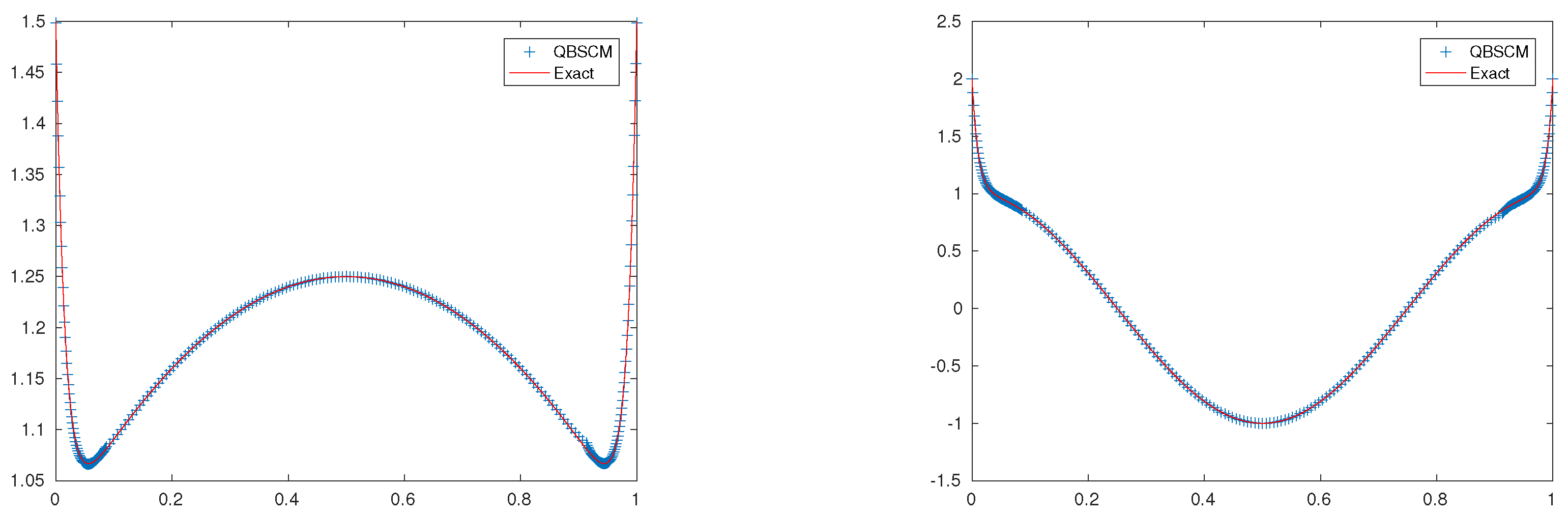
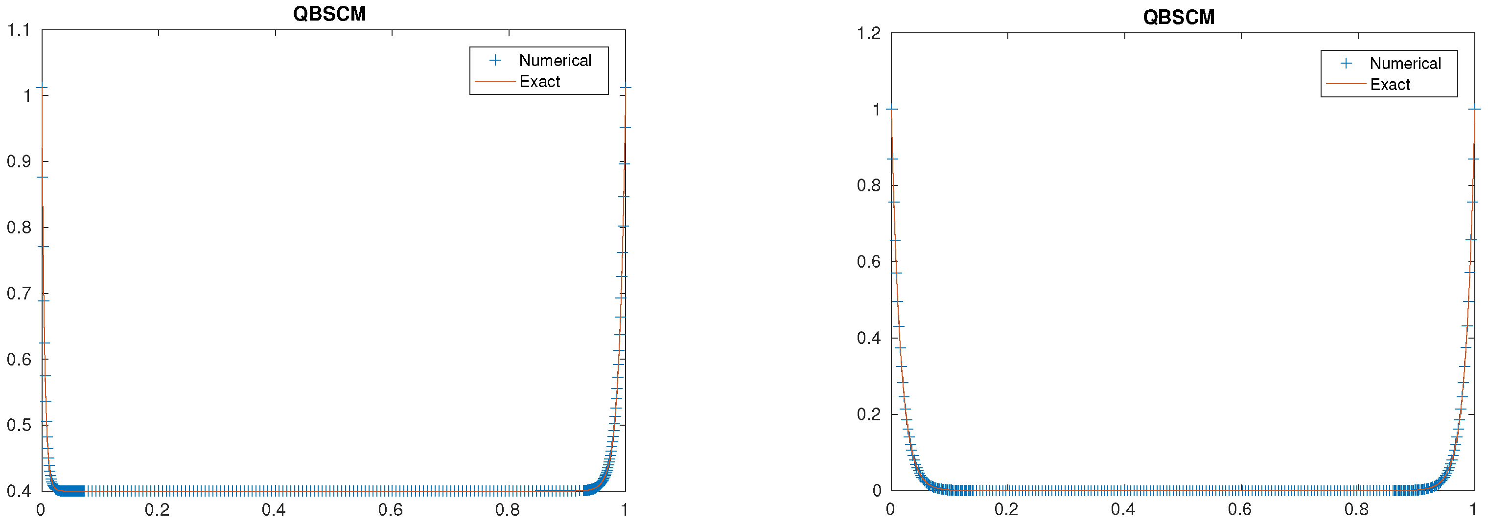
5. Numerical Experiments

To demonstrate the performance of the collocation method based on quintic B-splines in the previous section, we compared it with some existing methods: the hybrid finite difference scheme in [9] and the cubic spline scheme in [10]. Here, we apply the proposed numerical scheme to the test problems stated below:

Example 1.

$$\begin{array}{cc}\hfill & -{\epsilon }^2{u}^{\prime \prime }\left(x\right)-\epsilon (1+x)u^{\prime }\left(x\right)+3u\left(x\right)=f\left(x\right),x\in (0,1),\hfill \\ \hfill & u\left(0\right)=u\left(1\right),\epsilon (u^{\prime }\left(1\right)-u^{\prime }\left(0\right))=1-2\epsilon ,\hfill \end{array}$$

where $f\left(x\right)$ is chosen such that the exact solution is given by

$$\begin{array}{c}\hfill u\left(x\right)={\displaystyle \frac{e^{-\frac{x}{\epsilon }}+e^{-\frac{(1-x)}{\epsilon }}}{2(1-e^{-\frac{1}{\epsilon }})}}+x(1-x)+1.\end{array}$$

Example 2.

$$\begin{array}{cc}\hfill & -{\epsilon }^2{u}^{\prime \prime }\left(x\right)-2\epsilon (2+sin\left(2\pi x\right))u^{\prime }\left(x\right)+(1+cos\left(2\pi x\right))u\left(x\right)=f\left(x\right),x\in (0,1),\hfill \\ \hfill & u\left(0\right)=u\left(1\right),\epsilon (u^{\prime }\left(1\right)-u^{\prime }\left(0\right))=3,\hfill \end{array}$$

where $f\left(x\right)$ is chosen such that the exact solution is given by

$$\begin{array}{c}\hfill u\left(x\right)={\displaystyle \frac{e^{-\frac{3x}{2\epsilon }}+e^{-\frac{3(1-x)}{2\epsilon }}}{(1-e^{-\frac{3}{2\epsilon }})}}+cos\left(2\pi x\right).\end{array}$$

Example 3.

$$\begin{array}{c}\hfill -{\epsilon }^2{u}^{\prime \prime }\left(x\right)-2\epsilon u^{\prime }\left(x\right)+5u\left(x\right)=2,x\in (0,1),\\ \hfill u\left(0\right)=u\left(1\right),\epsilon (u^{\prime }\left(1\right)-u^{\prime }\left(0\right))=3.\end{array}$$

whose exact solution is given by

$$\begin{array}{cc}\hfill u\left(x\right)=& -3\left({\displaystyle \frac{e^{m_{1}x}}{\epsilon (1-e^{m_1})(m_1-m_2)}}\right)+3\left({\displaystyle \frac{e^{m_{2}x}}{\epsilon (1-e^{m_2})(m_1-m_2)}}\right)+{\displaystyle \frac{2}{5}},\hfill \\ \hfill m_1=& {\displaystyle \frac{-1-\sqrt{6}}{\epsilon }};m_2={\displaystyle \frac{-1+\sqrt{6}}{\epsilon }}.\hfill \end{array}$$

Example 4.

$$\begin{array}{cc}\hfill & -{\epsilon }^2{u}^{\prime \prime }\left(x\right)-\epsilon (1+x-x^2)u^{\prime }\left(x\right)+(2+x-x^2)u\left(x\right)=f\left(x\right),x\in (0,1),\hfill \\ \hfill & u\left(0\right)=u\left(1\right),\epsilon (u^{\prime }\left(1\right)-u^{\prime }\left(0\right))=2.\hfill \end{array}$$

where $f\left(x\right)$ is chosen such that the exact solution is given by

$$\begin{array}{c}\hfill u\left(x\right)={\displaystyle \frac{exp(-x/\epsilon )+exp(-(1-x)/\epsilon )}{(1-exp(-1/\epsilon \left)\right)}}.\end{array}$$

Let $u^N$ be a numerical approximation of the exact solution u on the mesh ${\Omega }^N$ where N is the number of mesh subintervals. For a finite set of values $\epsilon \in R_{\epsilon }=\{2^{-1},2^{-2},\dots ,2^{-20}\}$, we compute the maximum pointwise errors [26] by

$$E_{\epsilon }^N=\underset{x_k\in {\overline{\Omega }}_{\epsilon }^N}{max}\left|(u^N-u)\left(x_k\right)\right|,$$

and

$$E^N=\underset{\epsilon }{max}{E}_{\epsilon }^N.$$

From these quantities, the orders of convergence [26] are computed as

$$p^N={log}_2\left({\displaystyle \frac{E^N}{E^{2N}}}\right).$$

The computed errors $E^N$ and orders of convergence $p^N$ for the above examples using QBSCM are displayed in

Table 1. Values of $E^N$ and $p^N$ for Example 1 using various methods.

	Number of mesh points N
	32	64	128	256	512	1024
	Hybrid difference scheme in [9]
$E^N$	$1.994\times {10}^{-2}$	$7.425\times {10}^{-3}$	$2.613\times {10}^{-3}$	$8.774\times {10}^{-4}$	$2.833\times {10}^{-4}$	$8.862\times {10}^{-5}$
$p^N$	1.4252	1.5069	1.5742	1.6308	1.6768	—
	Cubic spline scheme [10]
$E^N$	$5.953\times {10}^{-2}$	$1.886\times {10}^{-2}$	$4.492\times {10}^{-3}$	$9.801\times {10}^{-4}$	$2.162\times {10}^{-4}$	$4.957\times {10}^{-5}$
$p^N$	1.6586	2.0695	2.1964	2.1806	2.1247	—
	QBSCM
$E^N$	$1.569\times {10}^{-2}$	$2.176\times -3$	$2.539\times {10}^{-4}$	$2.742\times {10}^{-5}$	$2.823\times {10}^{-6}$	$2.688\times {10}^{-7}$
$p^N$	2.8496	3.0996	3.2110	3.5799	3.8775	—

,

Table 2. Values of $E^N$ and $p^N$ for Example 2 using various methods.

	Number of mesh points N
	32	64	128	256	512	1024
	Hybrid difference scheme in [9]
$E^N$	$8.158\times {10}^{-1}$	$3.238\times {10}^{-1}$	$1.153\times {10}^{-1}$	$3.626\times {10}^{-2}$	$1.117\times {10}^{-2}$	$3.421\times {10}^{-3}$
$p^N$	1.3332	1.4901	1.6686	1.6986	1.7072	—
	Cubic spline scheme [10]
$E^N$	$4.276\times {10}^{-1}$	$8.577\times {10}^{-2}$	$2.270\times {10}^{-2}$	$5.793\times {10}^{-3}$	$1.447\times {10}^{-3}$	$3.571\times {10}^{-4}$
$p^N$	2.3179	1.9180	1.9701	2.0010	2.0189	—
	QBSCM
$E^N$	$7.471\times {10}^{-3}$	$1.004\times {10}^{-3}$	$1.162\times {10}^{-4}$	$1.278\times {10}^{-5}$	$1.293\times {10}^{-6}$	$5.589\times {10}^{-7}$
$p^N$	2.8963	3.1109	3.3837	3.5052	3.7471	—

,

Table 3. Values of $E^N$ and $p^N$ for Example 3 using various methods.

	Number of mesh points N
	32	64	128	256	512	1024
	Hybrid difference scheme in [9]
$E^N$	$9.743\times {10}^{-2}$	$4.136\times {10}^{-2}$	$1.597\times {10}^{-2}$	$5.694\times {10}^{-3}$	$1.906\times {10}^{-3}$	$6.089\times {10}^{-4}$
$p^N$	1.2360	1.3729	1.4880	1.5787	1.6465	—
	Cubic spline scheme [10]
$E^N$	$2.488\times {10}^{-1}$	$1.067\times {10}^{-1}$	$4.826\times {10}^{-2}$	$1.483\times {10}^{-2}$	$3.820\times {10}^{-3}$	$9.403\times {10}^{-4}$
$p^N$	1.2220	1.1442	1.7025	1.9565	2.0224	—
	QBSCM
$E^N$	$3.135\times {10}^{-1}$	$3.397\times {10}^{-2}$	$2.431\times {10}^{-3}$	$1.532\times {10}^{-4}$	$1.532\times {10}^{-4}$	$9.908\times {10}^{-6}$
$p^N$	3.2060	3.8047	3.9884	3.9504	3.9955	—

and

Table 4. Values of $E^N$ and $p^N$ for Example 4 using various methods.

	Number of mesh points N
	32	64	128	256	512	1024
	Hybrid difference scheme in [9]
$E^N$	$6.629\times {10}^{-1}$	$2.262\times {10}^{-1}$	$7.397\times {10}^{-2}$	$2.342\times {10}^{-2}$	$2.188\times {10}^{-3}$	$6.511\times {10}^{-4}$
$p^N$	1.5505	1.6096	1.6551	1.7222	1.7478	—
	Cubic spline scheme [10]
$E^N$	$3.503\times {10}^{-1}$	$1.036\times {10}^{-1}$	$2.724\times {10}^{-2}$	$7.113\times {10}^{-3}$	$1.816\times {10}^{-3}$	$4.538\times {10}^{-4}$
$p^N$	1.7577	1.9269	1.9372	1.9700	2.0005	—
	QBSCM
$E^N$	$3.974\times {10}^{-2}$	$3.456\times {10}^{-3}$	$2.266\times {10}^{-4}$	$1.390\times {10}^{-5}$	$8.703\times {10}^{-7}$	$5.642\times {10}^{-8}$
$p^N$	3.5234	3.9308	4.0274	3.9971	3.9471	—

. The results are compared with those obtained using the hybrid finite difference scheme in [9] and the cubic spline scheme in [10]. Figure 1 and Figure 2 display the exact and approximate solutions for the four problems, illustrating the boundary layers of the solutions. Additionally, Figure 3 and Figure 4 include log–log plots of the maximum absolute errors, confirming the convergent behavior of the proposed numerical method regardless of the perturbation values.

6. Conclusions

This work presented a numerical scheme based on a quintic B-spline collocation method for solving singularly perturbed convection–diffusion problems with periodic boundary conditions. Notably, the solutions to this type of problem exhibit boundary layers at both endpoints, $x=0$ and $x=1$. The Shishkin mesh was considered to carefully select the transition parameter, which plays a significant role in the scheme in accurately resolving the sharpness of the layers. The method was demonstrated to achieve fourth-order accuracy and was validated by solving four examples in which the errors were measured using the discrete maximum norm.

References

1. Miller, J.J.H.; O’Riordan, E.; Shishkin, G.I. Fitted Numerical Methods for Singular Perturbation Problems: Error Estimates in the Maximum Norm for Linear Problems in One and Two Dimensions; World Scientific Publishing Co. Pte. Ltd.: Singapore, 2012. [Google Scholar]
2. Farrell, P.A.; Hegarty, A.F.; Miller, J.J.H.; O’Riordan, E.; Shishkin, G.I. Robust Computational Techniques for Boundary Layers; Chapman and Hall/CRC: Boca Ration, FL, USA, USA, 2000. [Google Scholar]
3. Roos, H.G.; Stynes, M.; Tobiska, L. Robust Numerical Methods for Singularly Perturbed Differential Equations, Computational Mathematics; Springer: Berlin, Germany, 2008. [Google Scholar]
4. Kumar, D. A collocation method for singularly perturbed differential-difference turning point problems exhibiting boundary/interior layers. J. Differ. Equ. Appl. 2018, 24, 1847–1870. [Google Scholar] [CrossRef]
5. Puvaneswari, A. Valanarasu, T; Ramesh Babu, A. A System of Singularly Perturbed Periodic Boundary Value Problem: Hybrid Difference Scheme. Int. J. Appl. Comput. Math. 2020, 6, 86. [Google Scholar] [CrossRef]
6. Raja, V.; Geetha, N.; Mahendran, R.; Senthilkumar, L.S. Numerical solution for third order singularly perturbed turning point problems with integral boundary condition. J. Appl. Math. Comput. 2024, 1–21. [Google Scholar] [CrossRef]
7. Chandru, M.; Shanthi, V. A boundary value technique for singularly perturbed boundary value problem of reaction-diffusion with non-smooth data. J. Eng. Sci. Technol. Spec. Issue ICMTEA2013 Conf. 2014, 32–45. [Google Scholar]
8. Amiraliyev, G.M.; Duru, H. A uniformly convergence difference method for the periodical boundary value problem. Int. J. Comput. Math. Appl. 2003, 46, 695–703. [Google Scholar] [CrossRef]
9. Cen, Z. Uniformly convergent second-order difference scheme for a singularly perturbed periodical boundary value problem. Int. J. Comput. Math. 2011, 88, 196–206. [Google Scholar] [CrossRef]
10. Puvaneswari, A.; Ramesh Babu, A.; Valanarasu, T. Cubic spline scheme on variable mesh for singularly perturbed periodical boundary value problem. Novi Sad J. Math. 2020, 50, 157–172. [Google Scholar]
11. Kadalbajoo, M.K.; Patidar, K.C. A survey of numerical techniques for solving singularly perturbed ordinary differential equations. Appl. Math. Comput. 2002, 130, 457–510. [Google Scholar] [CrossRef]
12. Lang, F.G.; Xu, X.P. Quintic B-spline collocation method for second order mixed boundary value problem. Comput. Phys. Commun. 2012, 183, 913–921. [Google Scholar] [CrossRef]
13. Singh, S.; Kumar, D.; Shanthi, V. Uniformly convergent scheme for fourth-order singularly perturbed convection-diffusion ODE. Appl. Numer. Math. 2023, 186, 334–357. [Google Scholar] [CrossRef]
14. Singh, S.; Kumar, D. Spline-based parameter-uniform scheme for fourth-order singularly perturbed differential equations. J. Math. Chem. 2022, 60, 1872–1902. [Google Scholar] [CrossRef]
15. Yousaf, M.Z.; Srivastava, H.M.; Abbas, M.; Nazir, T.; Mohammed, P.O.; Vivas-Cortez, M.; Chorfi, N. A Novel quintic B-spline technique for numerical solutions of the fourth-order singular singularly-perturbed problems. Symmetry 2023, 15, 1929. [Google Scholar] [CrossRef]
16. Viswanadham, K.K.; Krishna, P.M. Quintic B-Spline Galerkin method for fifth order boundary value problems. ARPN J. Eng. Appl. Sci. 2010, 5, 74–77. [Google Scholar]
17. Mishra, H.K.; Lodhi, R.K. Two-parameter singular perturbation boundary value problems via quintic B-spline method. Proc. Natl. Acad. Sci. India Sect. A Phys. Sci. 2022, 92, 541–553. [Google Scholar] [CrossRef]
18. Micula, G. Handbook of Splines; Kluwer Academic Publishers: Dordrecht, The Netherlands, 1999. [Google Scholar]
19. Kumar, D. A parameter-uniform method for singularly perturbed turning point problems exhibiting interior or twin boundary layers. Int. J. Comput. Math. 2019, 96, 865–882. [Google Scholar] [CrossRef]
20. Kadalbajoo, M.K.; Yadaw, A.S.; Kumar, D. Comparative study of singularly perturbed two-point BVPs via: Fitted mesh finite difference method, B-spline collocation method. Appl. Math. Comput. 2008, 204, 713–725. [Google Scholar]
21. Puvaneswari, A.; Valanarasu, T. Spline approximation methods for second order singularly perturbed convection-diffusion equation with integral boundary condition. Indian J. Pure Appl. Math. 2024, 1–12. [Google Scholar] [CrossRef]
22. Chandru, M.; Shanthi, V. An asymptotic numerical method for singularly perturbed fourth order ODE of convection-diffusion type turning point problem. Neural Parallel Sci. Comput. 2016, 24, 473–488. [Google Scholar]
23. De Boor, C. A Practical Guide to Splines; Springer: New York, NY, USA, 1978. [Google Scholar]
24. Hall, C.A. On error bounds for spline interpolation. J. Approx. Theory I 1968, 209–218. [Google Scholar] [CrossRef]
25. Kadalbajoo, M.K.; Patidar, K.C. ε-Uniform fitted mesh finite difference methods for general singular perturbation problems. Appl. Math. Comput. 2006, 179, 248–266. [Google Scholar]
26. Chandru, M.; Shanthi, V. A Schwarz method for fourth-order singularly perturbed reaction-diffusion problem with discontinuous source term. J. Appl. Math. Inform. 2016, 34, 495–508. [Google Scholar] [CrossRef]
Figure 1. Exact and numerical solutions of Example 1 (left) and Example 2 (right) obtained using QBSCM for ε = 2 6 with N = 256 .
Axioms 14 00073 g001
Figure 2. Exact and numerical solutions of Example 3 (left) and Example 4 (right) obtained with QBSCM for ε = 2 6 with N = 256 .
Axioms 14 00073 g002
Figure 3. Log−log plot of the max error of Example 1 (left) and Example 2 (right) obtained using QBSCM for different ε values with N = 32 , 64 , 128 , 256 , 512 , 1024 .
Axioms 14 00073 g003
Figure 4. Log−log plot of the max error of Example 3 (left) and Example 4 (right) obtained with QBSCM for different ε values with N = 32 , 64 , 128 , 256 , 512 , 1024 .
Axioms 14 00073 g004