Parameters Determination via Fuzzy Inference Systems for the Logistic Populations Growth Model

Abstract

This study addresses the fuzzy parameters (coefficient) determination for the logistic population growth model, proposing a novel methodology based on fuzzy logic concepts. Population dynamics are often modeled using differential equations whose parameters represent critical ecological information, where the parameters determination is a problem itself. Unlike those approaches, the proposed methodology leverages ecosystem variables as inputs to a fuzzy inference system, which then generates fuzzy coefficients that better capture the inherent uncertainties in population dynamics. The approach was tested on a case study involving marine fish populations, where the fuzzy coefficients for growth rate and carrying capacity were calculated and integrated into the logistic model. The results illustrate that the fuzzy model with the proposed coefficients provide a robust framework for modeling population growth, preserving the increasing trajectory of the population under different scenarios. This method allows for the incorporation of expert knowledge and linguistic variables into the model, offering a more flexible and accurate representation of real-world ecosystems. The study concludes that this methodology significantly enhances the model’s applicability and predictive power, particularly in situations where precise data are not available.

1. Introduction

Mathematical modeling plays a crucial role in understanding various natural phenomena. One of the well-established areas within mathematical modeling is population growth dynamics, where models help to predict and analyze the behavior of populations over time [1]. Among the most notable models in this field is the Verhulst logistic model, which describes population growth by considering both exponential growth and the limitations imposed by environmental factors. The Verhulst equation has been widely applied to real-world problems, providing valuable insights into ecological systems and population dynamics [2,3]. This model is particularly useful when studying populations constrained by resources, as it introduces the concept of carrying capacity, which is the maximum population size that an environment can sustain [4,5,6].

The main tool to model these kind of phenomena are the differential equations (DEs). Nevertheless, in many practical scenarios, the parameters that define these differential equations, such as growth rate and carrying capacity, are not precisely known due to data variability or measurement uncertainties. To address this issue, fuzzy differential equations (FDEs) have been introduced, offering a robust mathematical framework for handling uncertainty in initial conditions and model parameters. The FDEs have been successfully applied to various fields, extending classical differential equations into the fuzzy domain, where uncertainties are represented by fuzzy numbers [7,8,9].

An extension of the Verhulst logistic model into the fuzzy domain, known as the fuzzy Verhulst model, allows for more realistic representations of populations where parameters, like growth rate and carrying capacity, are not fixed but vary within certain bounds [10]. This approach captures the inherent uncertainties in ecological systems, where factors such as resource availability or environmental conditions fluctuate over time [11]. The fuzzy Verhulst model thus provides a more flexible tool for population modeling especially when precise data are unavailable.

Parameter estimation in both classical and FDEs is a critical task, as the accuracy of the model heavily depends on the proper determination of these coefficients [12,13,14,15]. In the classical framework, statistical or numerical methods are often employed to estimate parameters based on historical data [16]. However, when dealing with fuzzy models, parameter estimation becomes more complex due to the uncertainty in both the data and the model structure itself. Several approaches, including fuzzy regression techniques, have been developed to estimate parameters in FDEs, such as the fuzzy least absolute regression model, which incorporates probabilistic linguistic term sets for handling fat-tailed or outlier-prone data [17], and the Intuitionistic Fuzzy Logistic Regression model, which deals with imprecise parameters due to vagueness and hesitation in datasets [18]. In [19], the authors introduce a fuzzy autoregression model to predict wind speed and direction. The model uses fuzzy numbers for regression coefficients, which effectively manage the inherent variability and uncertainty in wind patterns. These accurate predictions can enhance power system reliability by optimizing wind power integration into the grid.

As seen, most of the solution techniques for DEs in the domain of real numbers can be adapted and used in the study of the FDE. The calculation of coefficients for DE models can be divided into two main classes: (1) techniques using historical data and (2) techniques without using data. Numerical–statistical methods or evolutionary methods belong to the first class, and coefficients proposed by the expert are representative of the second.

As part of the fuzzy mathematics and systems theory, let us consider the concept of a fuzzy inference system (FIS), first introduced by Zadeh [20,21], that allows dealing with situations where the information is vague or imprecise and allows considering experts’ knowledge for the design of causal experts systems. A lot of theory has been developed around this type of system, as well as a large number of applications, some of which are related to control [22,23,24,25,26,27,28,29,30,31,32,33], forescasting [34,35,36,37,38], and classification [39,40,41,42,43], to name a few. These characteristics of the FIS are used to design the coefficients for the FDEs.

The motivation for this research stems from the need to develop an alternative method for estimating the coefficients of the fuzzy Verhulst model, specifically considering fuzzy coefficients, without relying on traditional datasets. The proposed approach leverages an FIS closely related to the phenomenon under study. By utilizing linguistic variables within the FIS and performing arithmetic operations, the model’s coefficients are calculated based entirely on expert knowledge. This methodology provides a robust alternative to numerical or statistical methods, which typically require large volumes of data and extensive processing time. Instead, it offers a practical solution that effectively models complex systems governed by well-defined rules, integrating fuzzy coefficients without requiring extensive data processing.

Therefore, the problem statement is centered on the estimation of fuzzy coefficients in the Verhulst model, which traditionally relies on large datasets and statistical methods. However, in scenarios where data are limited or unavailable, these traditional methods become impractical. Additionally, adapting fuzzy techniques to handle fuzzy coefficients without relying on data remains a significant challenge. This study addresses this issue by developing an approach based on an FIS that leverages expert knowledge to calculate the model’s coefficients, thereby eliminating the need for historical data.

The remainder of this paper is organized as follows: Section 2 is about the preliminaries; in Section 3, the materials and methods for the determination of fuzzy coefficients are presented; in Section 4, the results are shown; Section 5 presents the discussion; and in Section 6, the conclusions are stated.

2. Preliminaries

In this section, the main preliminaries are presented for the development of the rest of the article.

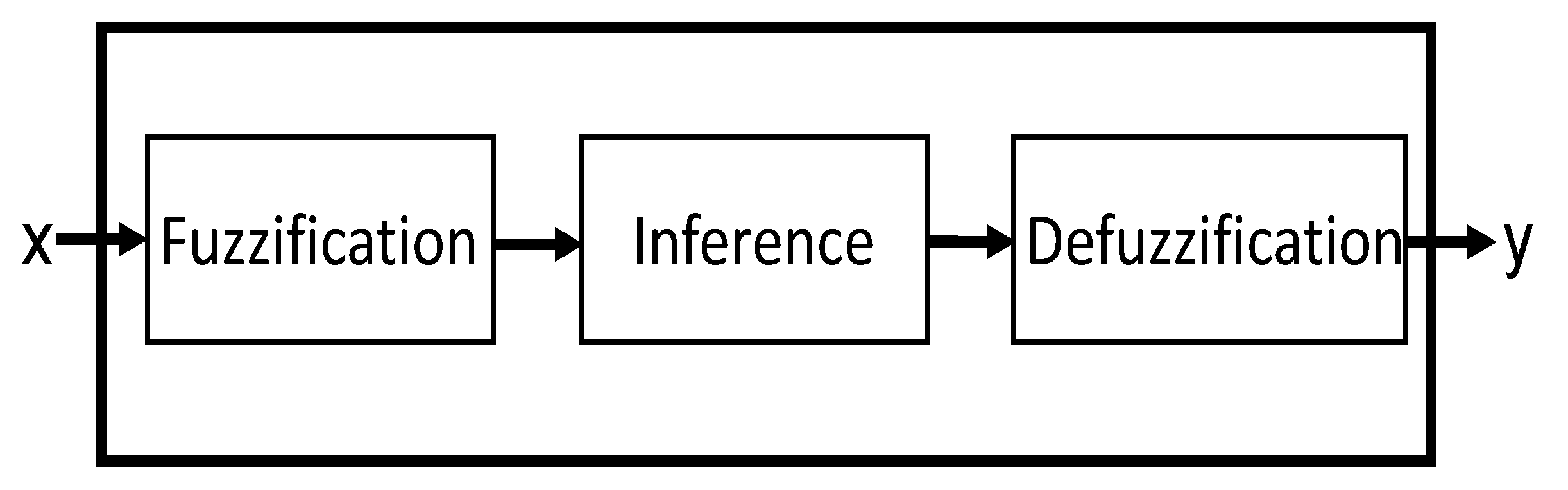
2.1. Necessary Knowledge About Fuzzy Inference Systems

Consider the following definitions:

Definition 1

([20]). A fuzzy set A is a tuple of two elements defined as $A=\left\{(x,{\mu }_A\left(x\right))\right|x\in \mathbb{R},{\mu }_A\left(x\right)\in [0,1]\}$, where ${\mu }_A\left(x\right)$ is the membership function of the fuzzy set A.

So, the membership function is defined as

Definition 2

([20]). Given X any set. The membership function ${\mu }_A$ of a non-empty fuzzy set A is a function ${\mu }_A:X\to [0,1]$. The function ${\mu }_A$ is interpreted as the degree of membership of each element x to the fuzzy set A for each $x\in X$.

The $\alpha -cut$ operation is very useful because it allows writing some fuzzy sets in intervals, and in this way, it is easier to execute arithmetic operations [44]. The $\alpha -cut$ operation of a fuzzy set A denoted by ${\left[A\right]}^{\alpha }$ is defined as

Definition 3

([20]). Let $\mu :\mathbb{R}\to [0,1]$, the membership function of a fuzzy set over $\mathbb{R}$, the $\alpha -cut$ or $\alpha -level$ is defined as the set ${\left[A\right]}^{\alpha }=\left\{x\in \mathbb{R}:{\mu }_A\left(x\right)\ge \alpha \right\}$ for each $0<\alpha \le 1$.

In the context of fuzzy systems, the inaccurate or uncertain information can be represented as a linguistic variable (LV). An LV is characterized by a tuple $(N,T,M,U)$, in which N is the name of the variable; T is the set of linguistic labels (each label is represented by a fuzzy set); M is the set of semantic rules that assign each label its meaning; and U is a universe of discourse (finite or infinite set).

Linguistic variables are important concepts in fuzzy logic, these variables are part of the FIS, and the FIS is a well-studied and applied form of knowledge representation.

The LVs are constituted by linguistic labels that allow the association of linguistic meaning to subintervals in the domain of each variable. A variable can have one or more linguistic labels; mathematically, these are represented through membership functions and consequently by fuzzy sets.

An FIS in general is a multivalued function where the inputs correspond to outputs and the function that makes this relationship is based on rules [45].

Specifically, the FIS has an inference engine that is responsible for performing the operations that relate to the inputs and outputs. Within this inference machine, there are three main modules (see Figure 1).

Fuzzification is the process of converting crisp, precise inputs into degrees of membership for fuzzy sets. The goal here is to map input values into fuzzy sets, where each fuzzy set represents a linguistic variable, for example, low, medium or high.

The inference engine processes the fuzzified inputs and applies fuzzy logic rules to produce fuzzy outputs. These rules are typically in the form of IF–THEN statements and operate on the fuzzified input data.

Defuzzification is the process of converting the fuzzy output obtained from the inference module into a crisp, actionable value. This step translates fuzzy conclusions into a real-world decision or action so that the output of this module is the output of the FIS itself.

There are several types of FIS, the more known are Takagi–Sugeno [46], Tsukamoto [47] and Mamdani [48]. A Mamdani-type fuzzy inference system (MFIS) is represented as a 4-tuple $M=(I,R,O,f)$ where the following apply:

• I is the set of linguistic variables of the inputs;
• R set of rules that relate the inputs to outputs;
• O set of linguistic variables of the outputs;
• f is a defuzzification method.

The relationship between the input and output linguistic variables is made through IF–THEN rules. These rules have the following form:

$$R_i:\mathrm{IF} x_1 \mathrm{is} M_{p1},x_2 \mathrm{is} M_{p2},\dots ,x_n \mathrm{is} M_{pk},\mathrm{THEN}{y}_1 \mathrm{is} N_{l1},y_2 \mathrm{is} N_{l2},\dots ,y_m \mathrm{is} N_{lj},$$

(1)

where $R_1,R_2,\dots ,R_i\in R$ represents the rules; $x_1,x_2,\dots ,x_n\in I$ are the linguistic variables of the inputs; $M_{p1},M_{p2},\dots ,M_{pk}$ are the labels of the input variables; $y_1,y_2,\dots ,y_m\in O$ are the output variables and $N_{l1},N_{l2},\dots ,N_{lj}$ are their respective linguistic labels [49].

There are various defuzzification methods. The most used are the center of area, bisector of area, last of maximum, first of maximum, middle of maximum and weighted average [50].

2.2. Foundations on Fuzzy Differential Equations

In this section, definitions to generalize the concept of derivatives and elements to solve FDEs are presented. The definition of a fuzzy number is presented to move toward the derivative definition.

Definition 4

([51]). Let μ be the membership function of a fuzzy set. It is said that μ is a fuzzy number if $\mu :\mathbb{R}\to [0,1]$ and satisfies the following conditions:

(i) 

μ is normal; i.e., there exists al least one $x^{*}\in \mathbb{R}$ such that $\mu \left(x^{*}\right)=1$;

(ii) 

${\left[\mu \right]}^{\alpha }$ is closed $\forall \alpha \in (0,1]$; and

(iii) 

${\left[\mu \right]}^0$ is bounded.

One way to obtain better representations and be able to operate fuzzy numbers arithmetically is through interval algebra. Therefore, a fuzzy number can be represented as an interval in the following way:

Definition 5

([52]). Given $\mu \left(x\right)$ with $x\in \mathbb{R}$ as the membership function of a fuzzy number, then there exist continuous functions ${\mu }_L\left(\alpha \right)$ and ${\mu }_R\left(\alpha \right)$ called, respectively, the left membership function and right membership function, such that

$$\mu \left(x\right)=[{\mu }_L\left(\alpha \right),{\mu }_R\left(\alpha \right)],\forall \alpha \in [0,1]$$

(2)

with ${\mu }_L\left(\alpha \right)\le {\mu }_R\left(\alpha \right)$.

For arithmetic intervals, it is possible to define the basic operations, where subindexes L and R represent the extreme left and right of the interval, respectively.

Definition 6

([44,53]). Given $[S_L,S_R]$ and $[T_L,T_R]$ arithmetic intervals, $\lambda \in \mathbb{R}$ (a scalar number), the following operations are defined:

(i) 

Addition:

$[S_L,S_R]+[T_L,T_R]=[S_L+T_L,S_R+T_R].$

(ii) 

Subtraction:

$[S_L,S_R]-[T_L,T_R]=[S_L-T_L,S_R-T_R].$

(iii) 

Reciprocal:

if $0\notin [S_L,S_R]$ then ${[S_L,S_R]}^{-1}=[1/S_L,1/S_R]$;

if $0\in [S_L,S_R]$ then ${[S_L,S_R]}^{-1}$ is undefined.

(iv) 

Multiplication:

$[S_L,S_R]·[T_L,T_R]=[U_L,U_R]$,

where:

$U_L=\min \left\{S_L·T_L,S_L·T_R,S_R·T_L,S_R·T_R\right\}$,

$U_R=\max \left\{S_L·T_L,S_L·T_R,S_R·T_L,S_R·T_R\right\}$.

(v) 

Division:

$[S_L,S_R]/[T_L,T_R]=[S_L,S_R]·{[T_L,T_R]}^{-1}$.

(vi) 

Multiplication by a scalar:

$\lambda [S_L,S_R]=[\lambda S_L,\lambda S_R].$

The definition of differentiability in the fuzzy sense was first introduced by [54] as

Definition 7

([54]). Let $u,v\in {\mathcal{F}}_{\mathbb{R}}$ (fuzzy number on reals). If there exists $w\in {\mathcal{F}}_{\mathbb{R}}$ such that $u=v\oplus w$, then w is called the H-difference of u and v, and it is denoted by $u\ominus v$.

Observe that ⊖ means the H-difference in this context, and ⊕ is the opposite of this. Fuzzy differentiability is based in terms of limits, similar to classical derivative, and it is defined as

Definition 8

([54]). Let $F:T\to {\mathcal{F}}_{\mathbb{R}}$ and $t_0\in T\subseteq \mathbb{R}$. The function F is said to be differentiable on $t_0$ if

(I) 

There exists an element $\dot{F}\left(t_0\right)\in {\mathcal{F}}_{\mathbb{R}}$ such that for all $h>0$ sufficiently close to zero, there exist $F(t_0+h)\ominus F\left(t_0\right)$, $F\left(t_0\right)\ominus F(t_0-h)$ and limits

$$\underset{h\to 0^{+}}{lim}{\displaystyle \frac{F(t_0+h)\ominus F\left(t_0\right)}{h}}=\underset{h\to 0^{+}}{lim}{\displaystyle \frac{F\left(t_0\right)\ominus F(t_0-h)}{h}}$$

are equal to $\dot{F}\left(t_0\right)$, or

(II) 

There exists an element $\dot{F}\left(t_0\right)\in {\mathcal{F}}_{\mathbb{R}}$ such that for all $h<0$ sufficiently close to zero, there exist $F(t_0+h)\ominus F\left(t_0\right)$, $F\left(t_0\right)\ominus F(t_0-h)$ and limits

$$\underset{h\to 0^{-}}{lim}{\displaystyle \frac{F(t_0+h)\ominus F\left(t_0\right)}{h}}=\underset{h\to 0^{-}}{lim}{\displaystyle \frac{F\left(t_0\right)\ominus F(t_0-h)}{h}}$$

are equal to $\dot{F}\left(t_0\right)$.

It should be noted that if F is differentiable in the first form (I), then it is not differentiable in the second form (II), and vice versa, which is summarized in the following theorem:

Theorem 1

([51]). Let $F:T\to {\mathcal{F}}_{\mathbb{R}}$, and ${\left[F\left(t\right)\right]}^{\alpha }=[F_L^{\alpha }\left(t\right),F_R^{\alpha }\left(t\right)]$, for each $\alpha \in [0,1]$. Then

(i) 

If F is differentiable from Form-I, then $F_L^{\alpha }\left(t\right)$ and $F_R^{\alpha }\left(t\right)$ are differentiable functions and

$${\left[\dot{F}\left(t\right)\right]}^{\alpha }=[\left({\dot{F}}_L^{\alpha }\left(t\right)\right),\left({\dot{F}}_R^{\alpha }\left(t\right)\right)],$$

(3)

or

(ii) 

If F is differentiable from Form-II then $F_L^{\alpha }\left(t\right)$ y $F_R^{\alpha }\left(t\right)$ are differentiable functions and

$${\left[\dot{F}\left(t\right)\right]}^{\alpha }=[\left({\dot{F}}_R^{\alpha }\left(t\right)\right),\left({\dot{F}}_L^{\alpha }\left(t\right)\right)]$$

(4)

where L and R are subindexes that represent the left and right extremes in interval algebra, respectively. The superindex α represents the function expressed in the α-cut.

The previous theorem constitutes a tool that allows writing the FDE in terms of standard equations in real numbers using the interval arithmetic. The way for doing this is through the equality of intervals, which can be seen in

Definition 9

([45]). Two intervals $[S_L,S_R]$ and $[T_L,T_R]$ are said to be equal if and only if $S_L=T_L$ and $S_R=T_R$.

Another definition that is important to resolve the FDE is the initial value problem:

Definition 10

([55]). Let us consider the first-order linear fuzzy differential equation $\dot{\tilde{x}}=\tilde{f}\left(\tilde{x}\right)$, where $\tilde{f}\left(\tilde{x}\right)$ is a fuzzy function of $\tilde{x}$, and $\dot{\tilde{x}}$ is the H-derivative of $\tilde{x}$; if an initial value $\tilde{x}\left(0\right)={\tilde{x}}_0$ is given, then this is a fuzzy initial value problem (FIVP).

2.3. Verhulst Logistic Model Expressed as Fuzzy Differential Equation

We assume the basic law of growth expressed as the form $\dot{x}=xf\left(x\right)$, where $x\in \mathbb{R}$ and $f\left(x\right)$ is some function [56,57]. If this function is sufficiently smooth, it can be represented with an approximation of $f\left(x\right)$ through the expansion of the Taylor series around $x=0$:

$$\begin{array}{c}\hfill f\left(x\right)\approx f\left(0\right)+{\displaystyle \frac{f^{\prime }\left(0\right)}{1!}}x+{\displaystyle \frac{f^{″}\left(0\right)}{2!}}{x}^2+\dots +{\displaystyle \frac{f^n\left(0\right)}{n!}}{x}^n,\end{array}$$

(5)

where $n\in \mathbb{N}$ [58,59,60]. Note that if in the Taylor series, only the constant term is kept, then from $\dot{x}=xf\left(x\right)=x\left(f\left(0\right)\right)=rx$ is obtained exactly the equation $\dot{x}=rx$, where $r=f\left(0\right)$, and it is known as the growth rate. This equation means that the population growth is proportional to the r coefficient; this is named the Malthus equation [61,62,63]. If two terms of the Taylor series expasion are kept, then the equation $\dot{x}=xf\left(x\right)=x(f\left(0\right)+f^{\prime }\left(0\right)x)=rx\left(1-{\displaystyle \frac{x}{C}}\right)$ is obtained, which is the logistic equation, where $f\left(0\right)$ and $f^{\prime }\left(0\right)$ are connected to r and C, respectively, and the parameter C is the carrying capacity.

With this aim in mind, the classic Verhulst logistic model within the real domain has been discussed. But there are several ways to represent this model or any other as an FDE. In this work, all the coefficients of the model are considered as fuzzy numbers such that the model can be seen as

$$\dot{\tilde{x}}=\tilde{r}\tilde{x}\left(\tilde{1}-{\displaystyle \frac{\tilde{x}}{\tilde{C}}}\right),$$

(6)

where $\tilde{x},\tilde{r},\tilde{C}\in {\mathcal{F}}_{\mathbb{R}}$ and the fuzzy numbers are represented with a tilde above.

On the other hand, when Theorem 1 is applied, it can be represented (6) with interval algebra as

$$[{\dot{x}}_L,{\dot{x}}_R]=[r_L,r_R][x_L,x_R]\left([1,1]-{\displaystyle \frac{[x_L,x_R]}{[C_L,C_R]}}\right).$$

(7)

The subindex L and R represent the extremes of the left and right intervals, respectively [64].

3. Determination of Fuzzy Coefficients

For solving the problem stated, the following methodology is defined.

Let an FIS describe population dynamics, then the FIS makes up the input for the methodology. For this, the FIS can be taken from one previously built. Then, using the linguistic variables of the inputs, it is necessary to propose the modeling functions to calculate the coefficients $\tilde{r}$ and $\tilde{C}$ in (6). So, this section will also show the structure for the modeling functions. The diagram in Figure 2 represents the methodology to build $\tilde{r}$ and $\tilde{C}$ coefficients. For better understanding, the diagram was divided into stages.

In the input stage, it is necessary to have an FIS related to the model whose coefficients will be calculated. Therefore, the FIS must be made up of linguistic variables corresponding to the case study.

Considering the input, as step 1, it is established that the selection process consists of the following. From the linguistic variables in the FIS, the expert has to choose which of these variables are relevant for the construction of the coefficients. The relevance criterion can be based on modeling in real numbers or on the expert knowledge. The selected variables will be denoted as set E.

Step 2 consists of classifying the variables from step 1 into two subsets according to the expert knowledge about which variables could be important in the design of a specific coefficient. Therefore, each subset contains the linguistic variables to design each coefficient. These subsets will be denoted as $E_i$, where $E_{i\in \{r,c\}}$ is the subset of linguistic variables corresponding to each coefficient as a result of this step.

In step 3, the modeling functions are designed by the expert from the sets obtained in step 2. For this, a structure of modeling functions for calculating $\tilde{r}$ and $\tilde{C}$ is proposed as

$$\tilde{r}={\tilde{f}}_r\left(E_r\right)$$

(8)

and

$$\tilde{C}={\tilde{f}}_c\left(E_c\right),$$

(9)

where ${\tilde{f}}_r$ and ${\tilde{f}}_c$ are fuzzy functions that the expert must propose depending on the nature of the problem under study. These functions receive $E_i$ as a parameter, where $E_i$ is the set of linguistic variables determined in step 2 of the methodology.

As step 4, the modeling functions are evaluated with $E_i$ from the previous step.

Finally, numerical values for the coefficients are obtained in the output stage. The methodology presented for determining fuzzy coefficients offers significant advantages, particularly in handling the inherent uncertainties of ecological data. Traditional methods often rely on precise data, which can be difficult to obtain or may not accurately reflect the variability found in real-world scenarios. In contrast, our approach leverages expert knowledge through an FIS, enabling the integration of linguistic variables directly related to the phenomenon under study. This not only enhances the flexibility and robustness of the logistic growth model but also introduces a novel way of addressing data imprecision in population dynamics. By proposing fuzzy coefficients, it provides a framework that better captures the complexities and uncertainties of real ecosystems, thus improving the model’s applicability and predictive power in diverse environmental contexts.

An example will be presented in the next section.

4. Experimental Results

This case study will show how to determine the fuzzy coefficients for the logistic model using the methodology above described. For this, it will be using an FIS, and the model to calculate its coefficients is (6). This FIS is taken from [65], and it estimates the intrinsic extinction vulnerabilities of marine fishes to fishing. The FIS’s linguistic variables are used to design the functions ${\tilde{f}}_r$ and ${\tilde{f}}_c$ and therefore calculate the coefficients $\tilde{r}$ and $\tilde{C}$, respectively. Finally, the coefficients will be incorporated into (6), and this will be solved using an initial condition.

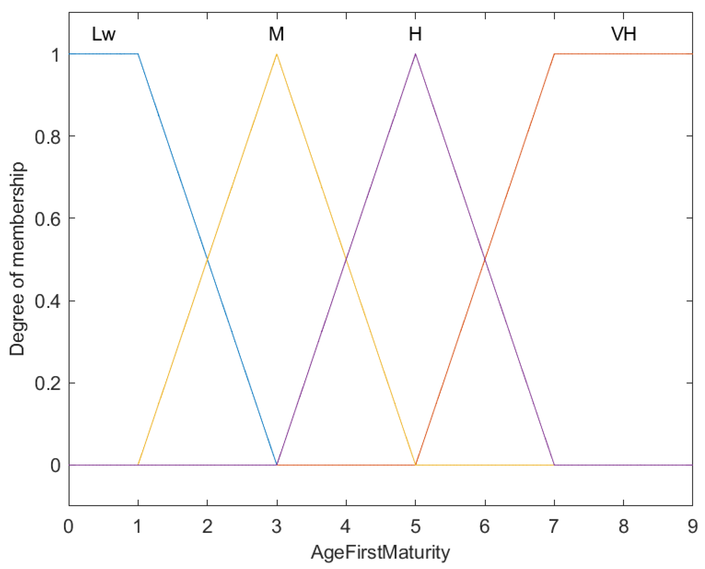
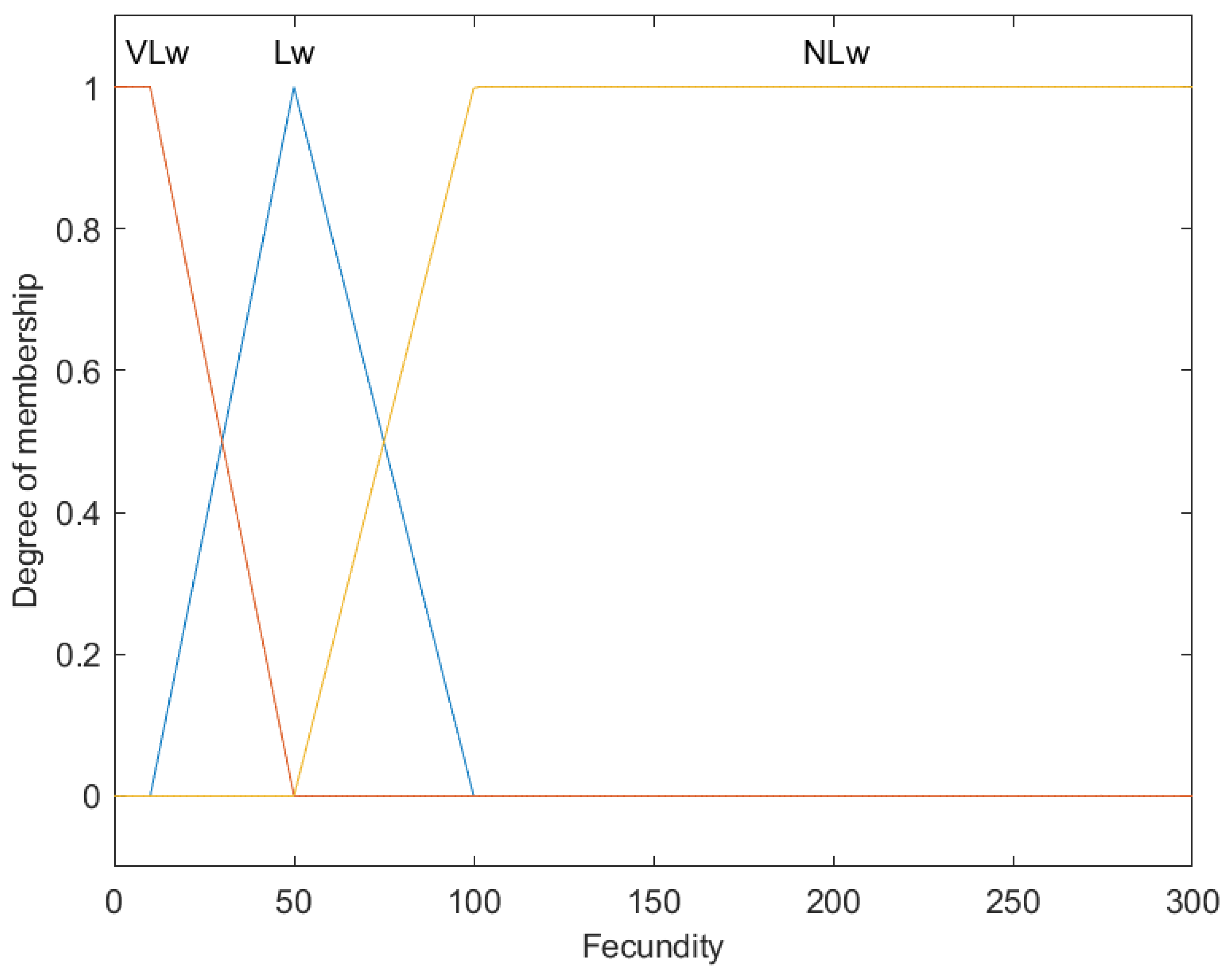
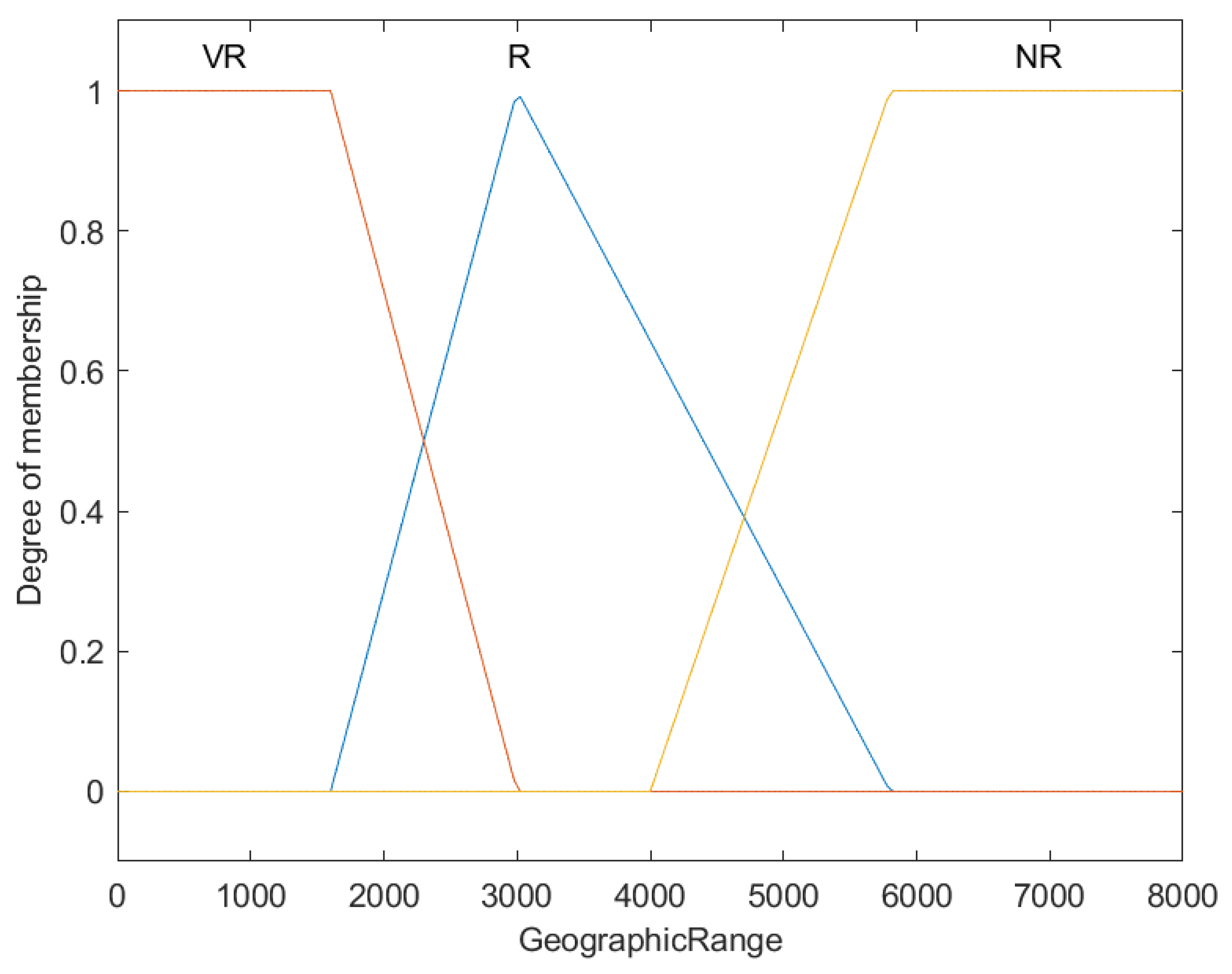
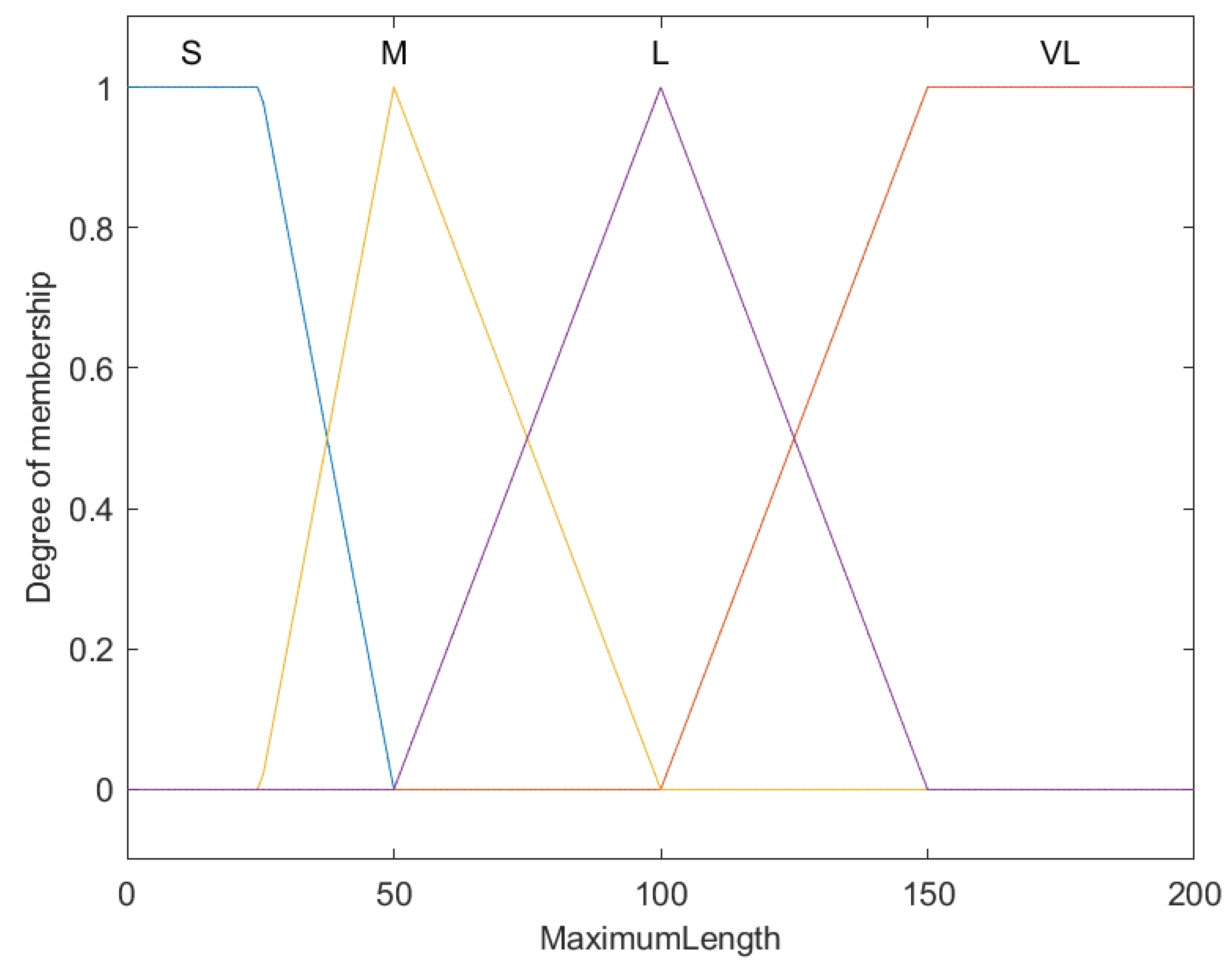
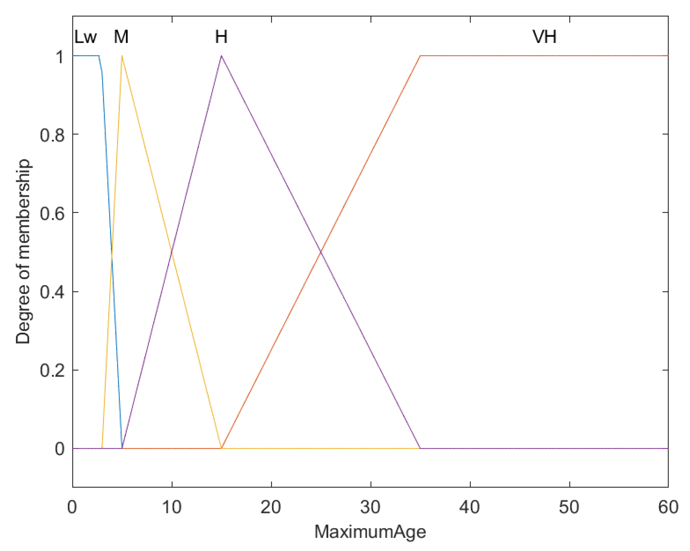
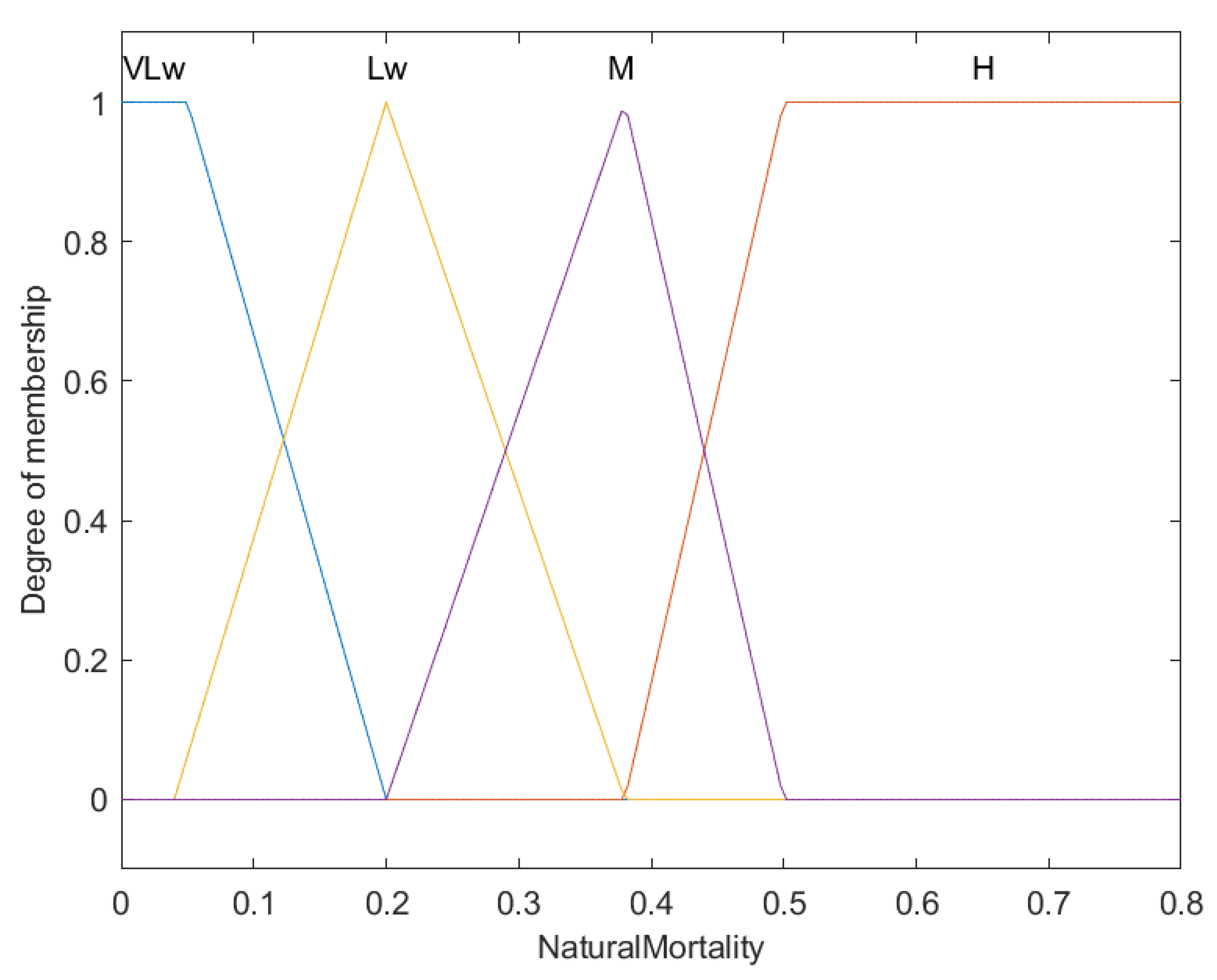
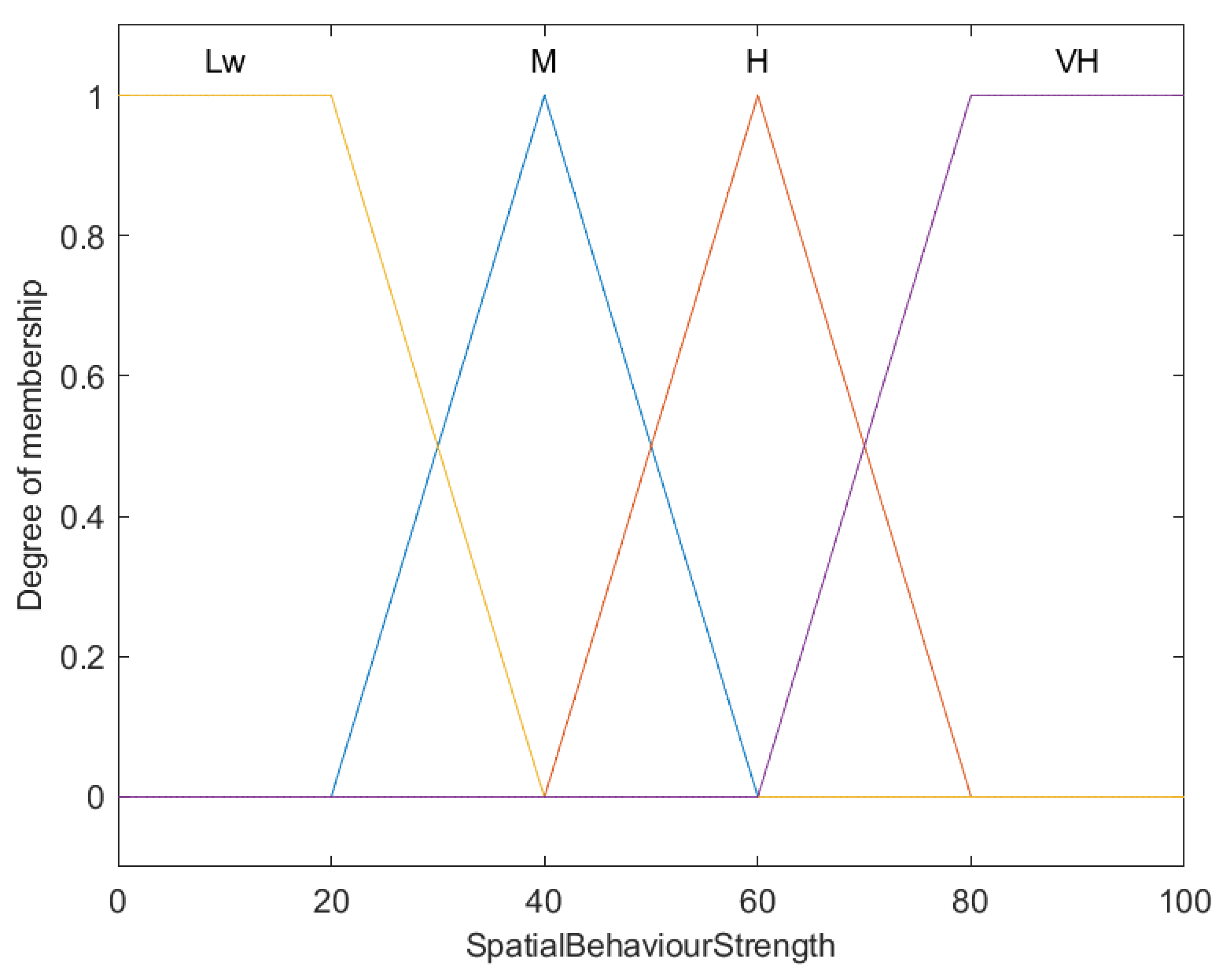
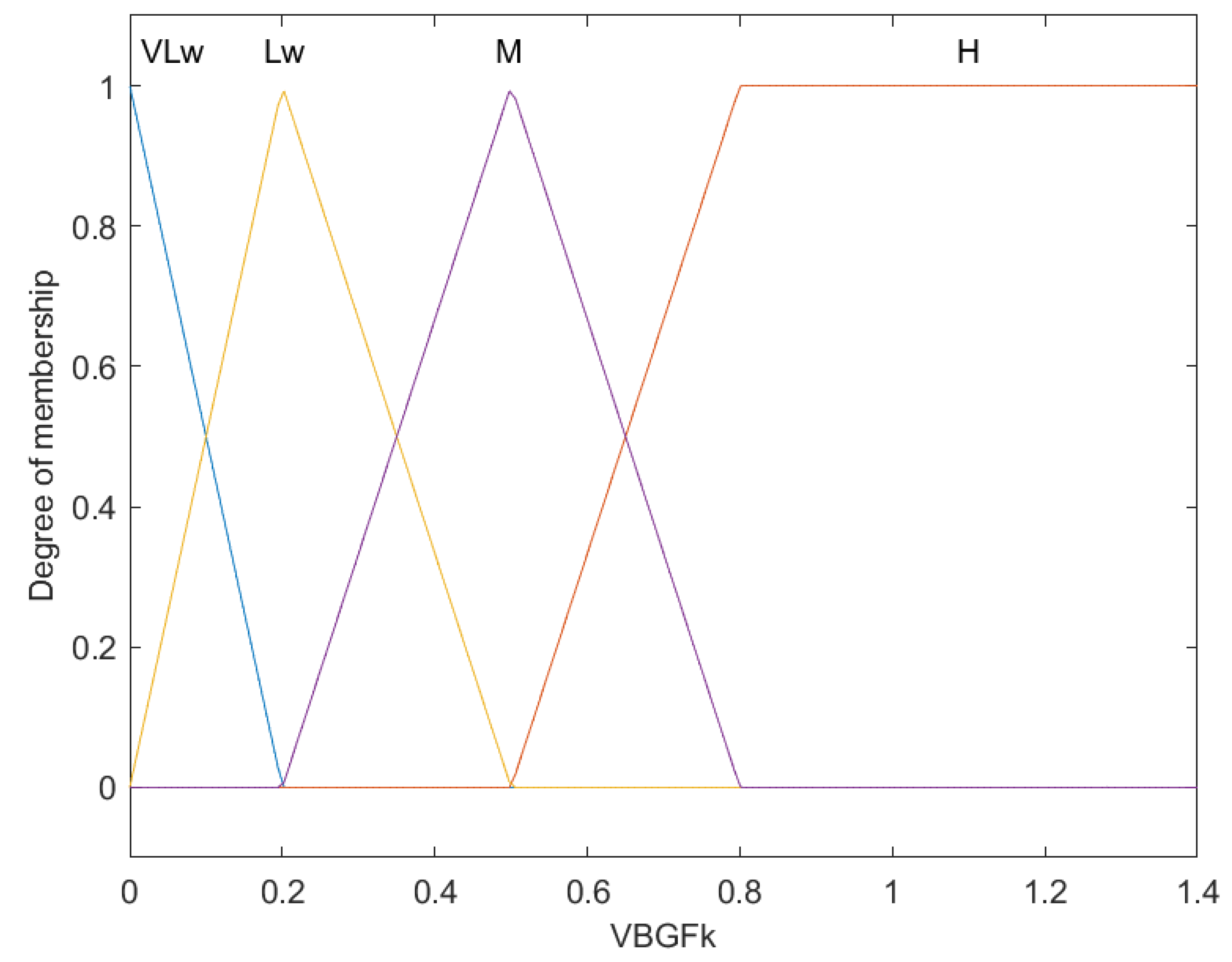
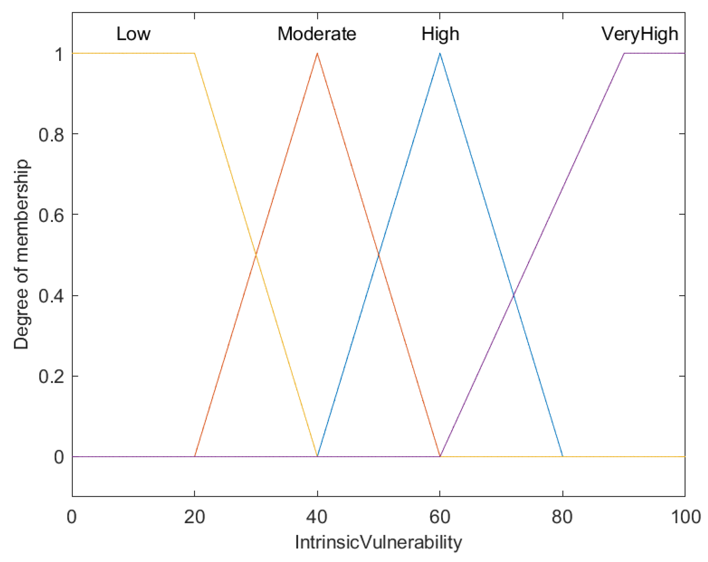
4.1. FIS That Estimates Vulnerabilities of Marine Fishes

In their study, the authors of [65] aimed to address the timely identification of vulnerable species for conservation efforts, despite incomplete information on most species that makes it challenging to establish an index of extinction vulnerability. To overcome this challenge, the authors developed a fuzzy inference system that assesses the intrinsic vulnerability of marine fishes. This system considers the fish’s life history and ecological traits, which contribute to their susceptibility to fishing. The maximum rate of population growth and strength of density dependence are important factors in assessing intrinsic vulnerability. Using life history and ecological characteristics as “rules-of-thumb”, the authors identified certain relationships commons for all species, and using that knowledge, the fuzzy system was developed.

The FIS developed in [65] is of the Mamdani type. This has eight inputs and one output, which are presented in Figure 3, Figure 4, Figure 5, Figure 6, Figure 7, Figure 8, Figure 9, Figure 10 and Figure 11, where Figure 3, Figure 4, Figure 5, Figure 6, Figure 7, Figure 8, Figure 9 and Figure 10 corresponds to the input variables and Figure 11 corresponds to the output variable. The defuzzification method used is the weighted average [66]. The rules are shown in

Table 1. Heuristic rules defined in the fuzzy system to assign relative vulnerabilities to fishes.

Rule		Conditions		Consequences
1	IF	Maximum length is very large	THEN	Vulnerability is very high
2	IF	Maximum length is large	THEN	Vulnerability is high
3	IF	Maximum length is medium	THEN	Vulnerability is moderate
4	IF	Maximum length is small	THEN	Vulnerability is low
5	IF	Age at first maturity is very high	THEN	Vulnerability is very high
6	IF	Age at first maturity is high	THEN	Vulnerability is high
7	IF	Age at first maturity is medium	THEN	Vulnerability is moderate
8	IF	Age at first maturity is low	THEN	Vulnerability is low
9	IF	Maximum age is very high	THEN	Vulnerability is very high
10	IF	Maximum age is high	THEN	Vulnerability is high
11	IF	Maximum age is medium	THEN	Vulnerability is moderate
12	IF	Maximum age is low	THEN	Vulnerability is low
	IF	VBGF K is very low	OR
13	IF	Natural mortality is very low	THEN	Vulnerability is very high
	IF	VBGF K is low	OR
14	IF	Natural mortality is low	THEN	Vulnerability is high
	IF	VBGF K is medium	OR
15	IF	Natural mortality is medium	THEN	Vulnerability is medium
	IF	VBGF K is high	OR
16	IF	Natural mortality is high	THEN	Vulnerability is low
17	IF	Geographic range is restricted	THEN	Vulnerability is high
18	IF	Geographic range is very restricted	THEN	Vulnerability is very high
19	IF	Fecundity is low	THEN	Vulnerability is high
20	IF	Fecundity is very low	THEN	Vulnerability is very high
21	IF	Spatial behaviour strength is low	THEN	Vulnerability is low
22	IF	Spatial behaviour strength is moderate	THEN	Vulnerability is moderate
23	IF	Spatial behaviour strength is high	THEN	Vulnerability is high
24	IF	Spatial behaviour strength is very high	THEN	Vulnerability is very high
25	IF	Spatial behaviour is related to feeding aggregation	THEN	Vulnerability resulted from spatial behaviour decreases
26	IF	Spatial behaviour is related to spawning aggregation	THEN	Vulnerability resulted from spatial behaviour increases

, and they are grouped according to the linguistic variable in the antecedent.

To construct the main linguistic variables that form the FIS, the article used as a reference is based on the biological and ecological characteristics of marine species, which are crucial for determining their intrinsic vulnerability to fishing. These characteristics include the maximum population growth rate, longevity, age at sexual maturity, and fecundity, among other parameters. These variables are combined using fuzzy set theory, which allows for the management of the inherent uncertainty in biological and ecological knowledge, as well as the challenges in strictly classifying species parameters. Fuzzy membership functions are employed to assign degrees of membership to different categories, such as low, medium or high, among others.

This figure illustrates the fuzzy membership functions for categorizing fish age at first maturity into four levels: Low (Lw), Medium (M), High (H), and Very High (VH). The X-axis represents the age at first maturity in years, while the Y-axis shows the membership degree from 0 to 1. Each color line corresponds to a category, demonstrating the gradual transitions and overlaps typical of fuzzy logic, which enables more nuanced classifications compared to binary categorization.

Depicted here are the fuzzy membership functions categorizing fish fecundity into three levels: Very Low (VLw), Low (Lw), and Not Low (NLw). On the X-axis, fecundity is quantified by the number of eggs, and the Y-axis represents the membership degree from 0 to 1. Each color represents a specific fecundity level, showcasing the utility of fuzzy logic for managing overlapping categories.

Illustrating the classification of fish geographic ranges, the graph uses fuzzy membership functions to sort ranges into Very Restricted (VR), Restricted (R), and Not Restricted (NR). The X-axis displays geographic range values in square kilometers, while the Y-axis assesses the membership degree, ranging from 0 to 1.

The graph delineates fuzzy membership functions that categorize the maximum length of fish into Small (S), Medium (M), Large (L), and Very Large (VL). The X-axis measures the maximum length in centimeters, and the Y-axis plots the membership degree from 0 to 1.

This graph categorizes the maximum age of fish using fuzzy membership functions across four classifications: Low (Lw), Medium (M), High (H), and Very High (VH). The X-axis presents the maximum age in years, and the Y-axis indicates the degree of membership, which is scaled from 0 to 1.

Portrayed in this graph are the fuzzy membership functions that segment natural mortality rates in fish into four categories: Very Low (VLw), Low (Lw), Medium (M), and High (H). The X-axis details the natural mortality rates per year, and the Y-axis reflects the membership degree from 0 to 1.

This graph elucidates the fuzzy membership functions applied to evaluate the spatial behavior strength of fish, which are segmented into four categories: Low (Lw), Medium (M), High (H), and Very High (VH). The X-axis represents the spatial behavior strength score, scaling from 0 to 100, while the Y-axis depicts the degree of membership, ranging from 0 to 1.

This chart illustrates the fuzzy membership functions used to categorize the von Bertalanffy growth factor (VBGFk) of fish, defining four levels: Very Low (VLw), Low (Lw), Medium (M), and High (H). The X-axis measures VBGFk values, while the Y-axis quantifies membership degrees from 0 to 1.

This graph presents the fuzzy membership functions that classify the intrinsic vulnerability of fish into four categories: Low, Moderate, High, and Very High. The X-axis depicts the intrinsic vulnerability score, ranging from 0 to 100, while the Y-axis represents the degree of membership from 0 to 1, as usual.

4.2. Proposal of Coefficients $\tilde{r}$ and $\tilde{C}$

The FIS presented in Section 4.1 will be the input for the methodology described in Section 3.

In step 1, the set of linguistic variables considered important to calculate the coefficients of the model under study is selected. The linguistic variables in

$$E=\{L_{max},T_m,K,M,T_{max},R,F\},$$

(10)

where $L_{max}$ means maximum length (for a fish); $T_m$ is the age at first maturity, K is the VBGF parameter (growth of fish [67]), M is the natural mortality rate, $T_{max}$ is the maximum age, R is the geographic range and F is the fecundity; all of them are features of a certain fish population, and these can be used in the calculation of the coefficients for the growth model.

Then, in step 2, the variables from the set E are classified as

$$E_r=\{T_m,K,M,T_{max},F\}$$

(11)

and

$$E_c=\{L_{max},R\}.$$

(12)

Note that in (11), the age at first maturity ($T_m$), natural growth (K), the natural mortality rate (M), the maximum age ($T_{max}$), and fecundity (F) are variables that directly influence r, which is similar to biological modeling rules on real numbers. In (12), variables such as $L_{max}$ means the maximum length of a fish’s body and R represents the geographic range; these are linked to the coefficient C.

Step 3 consists of designing the modeling functions (8) and (9); therefore, ${\tilde{f}}_r$ is proposed as the addition of natural growth, fecundity and the reciprocal of age at first maturity because those variables contribute to population growth; and the natural mortality rate and the reciprocal of maximum age are subtracted because they negatively influence the growth. The reciprocal expression for ${\tilde{T}}_m$ and ${\tilde{T}}_{max}$ is due to unit measure; observe, the before variables are in $year$ and the others are in $yea{r}^{-1}$. From this logic,

$$\tilde{r}={\tilde{f}}_r\left(E_r\right)=\tilde{K}+\tilde{F}+{\displaystyle \frac{1}{{\tilde{T}}_m}}-\tilde{M}-{\displaystyle \frac{1}{{\tilde{T}}_{max}}}$$

(13)

is designed.

Similarly to the real model, $\tilde{C}$ represents the carrying capacity in the ecosystem. Then,

$$\tilde{C}={\tilde{f}}_c\left(E_c\right)={\displaystyle \frac{\tilde{R}}{{\left(\frac{{\tilde{L}}_{max}}{100,000}\right)}^2}}$$

(14)

is explained as follows. The denominator expresses the square space required for a fish, where the constant 100,000 is a conversion factor between units of measurement. The idea is to know how many fishes can live in a certain region, and for this, it is necessary to divide $\tilde{R}$ between the space required for each fish. In this way, the ecosystem capacity is calculated.

As step 4 of the methodology, to evaluate (13) and (14) and obtain the outputs, a combination of linguistic labels is taken for the linguistic variables selected in (10).

Table 2. Linguistic labels for evaluate (13) and (14).

Linguistic Variables	Linguistic Labels	Values
$L_{max}$ (Maximum length)	S (Small)	$[0 50]$
$T_m$ (Age at first maturity)	Lw (Low)	$[0 3]$
K (von Bertalanffy growth parameter)	H (High)	$[0.5 1.4]$
M (Natural mortality rate)	H (High)	$[0.38 0.8]$
$T_{max}$ (Maximum age)	Lw (Low)	$[0 5]$
R (Geographic range)	NR (Not Restricted)	$[4000 8000]$
F (Fecundity)	NLw (Not Low)	$[50 300]$

presents the linguistic label together with the respective linguistic variable, and also the numeric value in interval form is shown. This combination of linguistic labels is chosen because it yields a low vulnerability value when it is evaluated in the FIS.

It is important to mention that each linguistic label is a fuzzy number, and these are used to obtain $\tilde{r}$ and $\tilde{C}$. When (13) and (14) are evaluated, then $\left[50.25300.60\right]$ and [1.63 326,530,612.24] are obtained, respectively, for $\tilde{r}$ and $\tilde{C}$ expressed as intervals.

4.3. Solutions for the Fuzzy Verhulst Logistic Model

To solve (7), it is necessary to consider an FIVP. Consider that the initial condition is [9,000,000 9,100,000], where X represents the number of fishes at a given time. Figure 12 shows the trajectories of the Form-I and Form-II solutions, ${\mathrm{X}}_{\mathrm{L}}$ and ${\mathrm{X}}_{\mathrm{R}}$ represent the extremes of the arithmetic interval corresponding to the solutions, and the green area is the uncertainty or membership value in the solutions.

All the calculations and solutions of the equation were programmed in a MatLab^® script (R2019a). Matlab’s ode45 numerical method is used to solve the model expressed as an FIVP.

The experimental results demonstrate the effectiveness of the proposed fuzzy coefficients in the logistic population growth model. The fuzzy model maintained stable and accurate growth trajectories, even under varying scenarios, highlighting its robustness in handling data uncertainties. Unlike traditional methods, this approach integrates expert knowledge without requiring extensive historical data, making it particularly useful in fields with limited or imprecise data. This shows that incorporating fuzzy logic enhances the model’s applicability and predictive power in complex environments.

5. Discussion

We used linguistic variables to evaluate the modeling functions. If, for example, the kernels are taken as representatives to evaluate numerically the FIS presented in Section 4.1, then we only need the value for the input corresponding to spatial behavior strength, because it was not used in the methodology. Even so, evaluating the FIS for the mentioned values and with all values on spatial behavior strength, the result of the intrinsic vulnerability index is in the range between 15.29 and 47.61; this means that the result is a low intrinsic vulnerability index. On the other hand, it can be appreciated that the solution curves for the model are increasing; here, an inversely proportional relationship can be established, given that when there is a low vulnerability, a population increase occurs.

6. Conclusions

In this work, a methodology for the construction of coefficients of Verhulst models expressed in differential equations was presented. The methodology was tested to calculate the fuzzy coefficients that represents the growth rate and the carrying capacity in the Verhulst model. The resolution of the Verhulst model that used the calculated coefficients and initial condition both defined as fuzzy numbers yielded a family of solutions that preserve the trajectories of increasing for the Form-I and Form-II solutions. It can be seen that there is an inverse relationship between the solutions and vulnerability with low vulnerability corresponding to a high growth.

The results obtained show that the proposed methodology to build coefficients, based on expert knowledge represented through fuzzy systems, could help to incorporate smoothly and easily the uncertainties and inaccuracies present in the parameters of the Verhulst model because the methodology is based on linguistic variables proposed by an expert that it is related to the nature of the model.

In comparison to existing models and methods for determining fuzzy coefficients, such as fuzzy regression techniques or evolutionary algorithms, the method applied in this study leverages a pre-existing FIS to calculate coefficients without relying extensively on large datasets. Traditional methods, such as statistical or evolutionary approaches, often require significant amounts of historical data, which can be limiting in ecological applications. In contrast, this study integrates the FIS from previous research, allowing for a flexible and adaptable calculation of fuzzy coefficients based on expert knowledge. While traditional methods are effective in certain contexts, the use of a pre-established FIS provides an efficient alternative for handling uncertainty and vagueness, particularly when precise data are not available.

This study offers valuable insights into the modeling of population dynamics using fuzzy logic, particularly in scenarios where precise data are unavailable or uncertainty is inherent. The methodology introduced for determining fuzzy coefficients in the logistic population growth model can be extended to a wide range of biomathematical applications, such as modeling species interactions, epidemiological models, and ecological sustainability assessments. By incorporating expert knowledge through FIS, this approach enhances the flexibility and realism of traditional population models, making it particularly useful in fields like conservation biology, ecological forecasting, and resource management, where accurate predictions are critical but data are often incomplete or imprecise.

Future work could explore the application of this methodology to other mathematical models in population dynamics, such as predator–prey models, age-structured population models, or spatial models that consider habitat fragmentation. Expanding beyond population dynamics, this approach could also be applied to fields like automatic control systems, where uncertainty plays a significant role in system behavior. By incorporating fuzzy logic into control theory models, such as in the regulation of biological processes or environmental systems, the robustness and adaptability of control mechanisms could be improved. Additionally, integrating this methodology with real-world case studies from both ecological and engineering fields could further validate its effectiveness and extend its utility across diverse scientific and industrial applications.

References

1. Banerjee, S. Mathematical Modeling: Models, Analysis and Applications; Chapman and Hall/CRC: Boca Raton, FL, USA, 2021. [Google Scholar]
2. Kalman, D. Verhulst Discrete Logistic Growth. Math. Mag. 2023, 96, 244–258. [Google Scholar] [CrossRef]
3. Morales-Erosa, A.; Reyes-Reyes, J.; Astorga-Zaragoza, C.M.; Osorio-Gordillo, G.L.; García-Beltrán, C.D.; Madrigal-Espinosa, G. Growth modeling approach with the Verhulst coexistence dynamic properties for regulation purposes. Theory Biosci. 2023, 142, 221–234. [Google Scholar] [CrossRef] [PubMed]
4. İskender, C. Mathematical Study of the Verhulst and Gompertz Growth Functions and Their Contemporary Applications. EKOIST J. Econom. Stat. 2021, 34, 73–102. [Google Scholar] [CrossRef]
5. Adeyeye, O.; Omar, Z. Investigating accuracy of multistep block methods based on step-length values for solving Malthus and Verhulst growth models. In AIP Conference Proceedings; AIP Publishing: Melville, NY, USA, 2022; Volume 2472. [Google Scholar]
6. Naso, P.; Lanz, B.; Swanson, T. The return of Malthus? Resource constraints in an era of declining population growth. Eur. Econ. Rev. 2020, 128, 103499. [Google Scholar] [CrossRef]
7. Zwillinger, D.; Dobrushkin, V. Handbook of Differential Equations; Chapman and Hall/CRC: Boca Raton, FL, USA, 2021. [Google Scholar]
8. Suhhiem, M.H. Legendre Operational Differential Matrix for Solving Fuzzy Differential Equations with Trapezoidal Fuzzy Function Coefficients. J. Kufa Math. Comput. 2024, 11, 31–48. [Google Scholar]
9. Thangathamizh, R. A Revised Fuzzy Differential Equations Using Weakly Compatible Self-Mappings in Revised Fuzzy Metric Spaces. Adv. Nonlinear Var. Inequalities 2024, 27, 233–254. [Google Scholar] [CrossRef]
10. Shiri, B.; Alijani, Z.; Karaca, Y. A power series method for the fuzzy fractional logistic differential equation. Fractals 2023, 31, 2340086. [Google Scholar] [CrossRef]
11. Cecconello, M.; Dorini, F.; Haeser, G. On fuzzy uncertainties on the logistic equation. Fuzzy Sets Syst. 2017, 328, 107–121. [Google Scholar] [CrossRef]
12. Ghosh, D.; Mandal, C. Clustering Based Parameter Estimation of Thyroid Hormone Pathway. IEEE/ACM Trans. Comput. Biol. Bioinform. 2022, 19, 343–354. [Google Scholar] [CrossRef] [PubMed]
13. Guan, Y.; Li, Y.; Ke, Z.; Peng, X.; Liu, R.; Li, Y.; Du, Y.P.; Liang, Z.P. Learning-Assisted Fast Determination of Regularization Parameter in Constrained Image Reconstruction. IEEE Trans. Biomed. Eng. 2024, 71, 2253–2264. [Google Scholar] [CrossRef]
14. Cui, J.; Chen, R.; Feng, F.; Wang, J.; Zhang, J.; Liu, W.; Ma, K.; Zhang, Q.J. Advanced Bayesian-Inspired Multilayer Effective Parameter Determination Method for Automated ANN Model Generation of Microwave Components. IEEE Trans. Microw. Theory Tech. 2024, 72, 4408–4420. [Google Scholar] [CrossRef]
15. He, P.; Liu, Y.; Zhang, B.; He, J. Determination of Parameters for Space Charge Simulation Based on Bipolar Charge Transport Model Under a Divergent Electric Field. IEEE Trans. Dielectr. Electr. Insul. 2024, 31, 1376–1385. [Google Scholar] [CrossRef]
16. Pardoe, I. Applied Regression Modeling; John Wiley & Sons: Hoboken, NJ, USA, 2020. [Google Scholar]
17. Jiang, L.; Liao, H. Mixed fuzzy least absolute regression analysis with quantitative and probabilistic linguistic information. Fuzzy Sets Syst. 2020, 387, 35–48. [Google Scholar] [CrossRef]
18. Ahmadini, A.A.H. A novel technique for parameter estimation in intuitionistic fuzzy logistic regression model. Ain Shams Eng. J. 2022, 13, 101518. [Google Scholar] [CrossRef]
19. Khasanzoda, N.; Zicmane, I.; Beryozkina, S.; Safaraliev, M.; Sultonov, S.; Kirgizov, A. Regression model for predicting the speed of wind flows for energy needs based on fuzzy logic. Renew. Energy 2022, 191, 723–731. [Google Scholar] [CrossRef]
20. Zadeh, L. Fuzzy sets. Inf. Control 1965, 8, 338–353. [Google Scholar] [CrossRef]
21. Zadeh, L. The concept of a linguistic variable and its application to approximate reasoning-I. Inf. Sci. 1975, 8, 199–249. [Google Scholar] [CrossRef]
22. Zhang, T.; Qu, H.; Zhou, J. Asymptotically almost periodic synchronization in fuzzy competitive neural networks with Caputo-Fabrizio operator. Fuzzy Sets Syst. 2023, 471, 108676. [Google Scholar] [CrossRef]
23. Cazarez-Castro, N.R.; Aguilar, L.T.; Castillo, O. Fuzzy logic control with genetic membership function parameters optimization for the output regulation of a servomechanism with nonlinear backlash. Expert Syst. Appl. 2010, 37, 4368–4378. [Google Scholar] [CrossRef]
24. Cazarez-Castro, N.R.; Aguilar, L.T.; Castillo, O. Designing Type-1 and Type-2 Fuzzy Logic Controllers via Fuzzy Lyapunov Synthesis for nonsmooth mechanical systems. Eng. Appl. Artif. Intell. 2012, 25, 971–979. [Google Scholar] [CrossRef]
25. Cazarez-Castro, N.R.; Aguilar, L.T.; Castillo, O.; Rodríguez-Dŕaz, A. Controlling Unstable Non-Minimum-Phase Systems with Fuzzy Logic: The Perturbed Case. In Evolutionary Design of Intelligent Systems in Modeling, Simulation and Control; Castillo, O., Pedrycz, W., Kacprzyk, J., Eds.; Springer: Berlin/Heidelberg, Germany, 2009; pp. 245–257. [Google Scholar] [CrossRef]
26. Miranda-Colorado, R.; Cazarez-Castro, N.R. Observer-based fuzzy trajectory-tracking controller for wheeled mobile robots with kinematic disturbances. Eng. Appl. Artif. Intell. 2024, 133, 108279. [Google Scholar] [CrossRef]
27. Herrera-Garcia, L.; Cazarez-Castro, N.R.; Cardenas-Maciel, S.L.; Lopez-Renteria, J.A.; Aguilar, L.T. Self-excited periodic motion in underactuated mechanical systems using two-fuzzy inference system. Fuzzy Sets Syst. 2022, 438, 25–45. [Google Scholar] [CrossRef]
28. Prieto, P.J.; Cazarez-Castro, N.R.; Aguilar, L.T.; Cardenas-Maciel, S.L. Chattering existence and attenuation in fuzzy-based sliding mode control. Eng. Appl. Artif. Intell. 2017, 61, 152–160. [Google Scholar] [CrossRef]
29. Cazarez-Castro, N.R.; Aguilar, L.T.; Cardenas-Maciel, S.L.; Goribar-Jimenez, C.A.; Odreman-Vera, M. Diseño de un Controlador Difuso mediante la Síntesis Difusa de Lyapunov para la Estabilización de un Péndulo de Rueda Inercial. Rev. Iberoam. de Automática e Inf. Ind. RIAI 2017, 14, 133–140. [Google Scholar] [CrossRef]
30. Prieto-Entenza, P.J.; Cazarez-Castro, N.R.; Aguilar, L.T.; Cardenas-Maciel, S.L.; Lopez-Renteria, J.A. A Lyapunov Analysis for Mamdani Type Fuzzy-Based Sliding Mode Control. IEEE Trans. Fuzzy Syst. 2020, 28, 1887–1895. [Google Scholar] [CrossRef]
31. Prieto, P.J.; Aguilar, L.T.; Cardenas-Maciel, S.L.; Lopez-Renteria, J.A.; Cazarez-Castro, N.R. Stability Analysis for Mamdani-Type Integral Fuzzy-Based Sliding-Mode Control of Systems Under Persistent Disturbances. IEEE Trans. Fuzzy Syst. 2022, 30, 1640–1647. [Google Scholar] [CrossRef]
32. Lopez-Renteria, J.A.; Herrera-Garcia, L.; Cardenas-Maciel, S.L.; Aguilar, L.T.; Cazarez-Castro, N.R. Self-Sustaining Oscillations With an Internal Two-Fuzzy Inference System Based on the Poincaré–Bendixson Method. IEEE Trans. Fuzzy Syst. 2022, 30, 2563–2573. [Google Scholar] [CrossRef]
33. Pulido–Luna, J.R.; López–Rentería, J.A.; Cazarez–Castro, N.R. Mamdani-Type Fuzzy-Based Adaptive Nonhomogeneous Synchronization. Complexity 2021, 2021, 9913114. [Google Scholar] [CrossRef]
34. Tang, Y.; Yu, F.; Zeng, W.; Ouyang, C.; Jiang, Y.; Liu, Y. Causalities-multiplicity oriented joint interval-trend fuzzy information granulation for interval-valued time series multi-step forecasting. Inf. Sci. 2025, 694, 121717. [Google Scholar] [CrossRef]
35. Li, F.; Wang, C. Polynomial fuzzy information granule based α-triple I fuzzy reasoning algorithm and its short-term forecasting of time series. Inf. Sci. 2025, 689, 121469. [Google Scholar] [CrossRef]
36. Xia, Y.; Wang, J.; Zhang, Z.; Wei, D.; Cao, Z.; Li, Z. A wind speed point-interval fuzzy forecasting system based on data decomposition and multiobjective optimizer. Appl. Soft Comput. 2024, 165, 112084. [Google Scholar] [CrossRef]
37. Xue, C.; Mahfouf, M. RACFIS: A New Rapid Adaptive Complex Fuzzy Inference System for Regression Modelling. IEEE Trans. Emerg. Top. Comput. Intell. 2024, 8, 1238–1252. [Google Scholar] [CrossRef]
38. Mei, Z.; Zhao, T.; Gu, X. A Dynamic Evolving Fuzzy System for Streaming Data Prediction. IEEE Trans. Fuzzy Syst. 2024, 32, 4324–4337. [Google Scholar] [CrossRef]
39. Salimi-Badr, A.; Parchamijalal, M.M. Self-organizing lightweight correlation-aware fuzzy broad learning system for high-dimensional large-scale classification problems. Appl. Soft Comput. 2025, 169, 112552. [Google Scholar] [CrossRef]
40. Ma, N.; Wu, K.; Yuan, Y.; Li, J.; Wu, X. PMWFCM: A Possibility based MultiKernel Weighted Fuzzy Clustering Algorithm for classification of driving behaviors. Alex. Eng. J. 2025, 113, 249–261. [Google Scholar] [CrossRef]
41. Wu, M.; Ma, L.; Fan, J. An expert classification consensus reaching model based on fuzzy trust relationship matrix in the application of steel industry. Expert Syst. Appl. 2025, 266, 126180. [Google Scholar] [CrossRef]
42. Zang, Z.S.; Yin, R.; Lu, W.; Pedrycz, W.; Zhang, L.Y. A Linguistically Interpretable Deep Fuzzy Classification System With Feature Transformation and Reconstruction. IEEE Trans. Fuzzy Syst. 2024, 32, 4297–4311. [Google Scholar] [CrossRef]
43. Zhang, X.; Chen, D.; Mi, J. Fuzzy Decision Rule-Based Online Classification Algorithm in Fuzzy Formal Decision Contexts. IEEE Trans. Fuzzy Syst. 2023, 31, 3263–3277. [Google Scholar] [CrossRef]
44. Young, R.E.G.R.E. A parametric representation of fuzzy numbers and their arithmetic operators. Fuzzy Sets Syst. 1997, 91, 185–202. [Google Scholar]
45. Chen, G.; Pham, T.T. Introduction to Fuzzy Systems; Chapman and Hall/CRC: Boca Raton, FL, USA, 2005. [Google Scholar]
46. Casillas, J.; Cordon, O.; Herrera, F.; Magdalena, L. Interpretability Issues in Fuzzy Modeling. In Interpretability Issues in Fuzzy Modeling; Springer: Berlin/Heidelberg, Germany, 2003; Volume 128, p. 643. [Google Scholar]
47. Gegov, A. Complexity Management in Fuzzy Systems: A Rule Base Compression Approach (Studies in Fuzziness and Soft Computing); Springer: Berlin/Heidelberg, Germany, 2007. [Google Scholar]
48. Sala, A.; Guerra, T.M.; Babuška, R. Perspectives of fuzzy systems and control. Fuzzy Sets Syst. 2005, 156, 432–444. [Google Scholar] [CrossRef]
49. Jang, J.S.R.; Sun, C.T. Neuro-Fuzzy and Soft Computing: A Computational Approach to Learning and Machine Intelligence; Prentice-Hall, Inc.: Dallas, TX, USA, 1996. [Google Scholar]
50. Trung Tat Pham, G.C. Introduction to Fuzzy Sets, Fuzzy Logic, and Fuzzy Control Systems; CRC Press: Boca Raton, FL, USA, 2000. [Google Scholar]
51. Kaleva, O. Fuzzy differential equations. Fuzzy Sets Syst. 1987, 24, 301–317. [Google Scholar] [CrossRef]
52. Dimuro, G.P. On Interval Fuzzy Numbers. In Proceedings of the 2011 Workshop-School on Theoretical Computer Science, Pelotas, Brazil, 24–26 August 2011; pp. 3–8. [Google Scholar]
53. Jorba, L.; Adillon, R. Interval Fuzzy Segments. Symmetry 2018, 10, 309. [Google Scholar] [CrossRef]
54. Ralescu, M.L.P.D.A. Differentials of fuzzy functions. J. Math. Anal. Appl. 1983, 91, 552–558. [Google Scholar]
55. Devi, S.S.; Ganesan, K. Application of linear fuzzy differential equation in day to day life. Aip Conf. Proc. 2019, 2112, 020169. [Google Scholar]
56. Fowler, A.C. Mathematical Models in the Applied Sciences; Cambridge University Press: Cambridge, UK, 1997; Volume 17. [Google Scholar]
57. Murray, J.D.; Murray, J.D. Mathematical Biology: II: Spatial Models and Biomedical Applications; Springer: Berlin/Heidelberg, Germany, 2003; Volume 3. [Google Scholar]
58. Fitzpatrick, P.M. Advanced Calculus, Pure and Applied Undergraduate Texts; American Mathematical Society: Providence, RI, USA, 2009; Volume 5. [Google Scholar]
59. Gillespie, R. Principles of Mathematical Analysis. By Walter Rudin. Pp. x, 227. 40s. 1953.(McGraw-Hill)-Theory of Functions of Real Variable. By Henry P. Thielman. Pp. xiv, 209. 35s. 1953. (Butterworth Scientific Publications, London). Math. Gaz. 1955, 39, 258–259. [Google Scholar] [CrossRef]
60. Pugh, C.C.; Pugh, C. Real Mathematical Analysis; Springer: Berlin/Heidelberg, Germany, 2002; Volume 2011. [Google Scholar]
61. Young, R.M. Malthus and the evolutionists: The common context of biological and social theory. Past Present 1969, 109–145. [Google Scholar] [CrossRef]
62. Cazarez-Castro, N.R.; Odreman-Vera, M.; Cardenas-Maciel, S.L.; Echavarria-Heras, H.; Leal-Ramirez, C. Fuzzy differential equations as a tool for teaching uncertainty in engineering and science. Comput. Sist. 2018, 22, 439–449. [Google Scholar] [CrossRef]
63. Cazarez-Castro, N.R.; Cardenas-Maciel, S.L.; Odreman-Vera, M.; Valencia-Palomo, G.; Leal-Ramirez, C. Modeling PD closed-loop control problems with fuzzy Differential Equations. Autom. Čas. Autom. Mjer. Elektron. Račun. Komun. 2016, 57, 960–967. [Google Scholar] [CrossRef]
64. Sorini, L.; Stefanini, L. Some Parametric Forms for LR Fuzzy Numbers and LR Fuzzy Arithmetic. In Proceedings of the 2009 Ninth International Conference on Intelligent Systems Design and Applications, Pisa, Italy, 30 November–2 December 2009; pp. 312–317. [Google Scholar]
65. Cheung, W.W.; Pitcher, T.J.; Pauly, D. A fuzzy logic expert system to estimate intrinsic extinction vulnerabilities of marine fishes to fishing. Biol. Conserv. 2005, 124, 97–111. [Google Scholar] [CrossRef]
66. Cox, E. The Fuzzy Systems Handbook: A Practitioners Guide to Building; AP Professional: Beaverton, OR, USA, 1994. [Google Scholar]
67. Pauly, D. On the interrelationships between natural mortality, growth parameters, and mean environmental temperature in 175 fish stocks. ICES J. Mar. Sci. 1980, 39, 175–192. [Google Scholar] [CrossRef]
Figure 1. Structure of an FIS.
Axioms 14 00036 g001
Figure 2. Methodology through modeling functions.
Axioms 14 00036 g002
Figure 3. Fuzzy membership functions for fish age at first maturity ( T m ).
Axioms 14 00036 g003
Figure 4. Fuzzy membership functions for fish fecundity (F).
Axioms 14 00036 g004
Figure 5. Fuzzy membership functions for geographic range of fish species (R).
Axioms 14 00036 g005
Figure 6. Fuzzy membership functions for maximum length of fish ( L m a x ).
Axioms 14 00036 g006
Figure 7. Fuzzy membership functions for maximum age of fish ( T m a x ).
Axioms 14 00036 g007
Figure 8. Fuzzy membership functions for natural mortality rates in fish (M).
Axioms 14 00036 g008
Figure 9. Fuzzy membership functions for spatial behavior strength in fish (B).
Axioms 14 00036 g009
Figure 10. Fuzzy membership functions for the natural growth (K).
Axioms 14 00036 g010
Figure 11. Fuzzy membership functions for intrinsic vulnerability (V).
Axioms 14 00036 g011
Figure 12. Form-I solution (left) and Form-II solution (right) for (7).
Axioms 14 00036 g012