Fractal Continuum Maxwell Creep Model

Abstract

In this work, the fractal continuum Maxwell law for the creep phenomenon is introduced. By mapping standard integer space-time into fractal continuum space-time using the well-known Balankin’s approach to variable-order fractal calculus, the fractal version of Maxwell model is developed. This methodology employs local fractional differential operators on discontinuous properties of fractal sets embedded in the integer space-time so that they behave as analytic envelopes of non-analytic functions in the fractal continuum space-time. Then, creep strain $\epsilon \left(t\right)$, creep modulus $J\left(t\right)$, and relaxation compliance $G\left(t\right)$ in materials with fractal linear viscoelasticity can be described by their generalized forms, ${\epsilon }^{\beta }\left(t\right),J^{\beta }\left(t\right) \mathrm{and} G^{\beta }\left(t\right)$, where $\beta =dimS/dimH$ represents the time fractal dimension, and it implies the variable-order of fractality of the self-similar domain under study, which are $dimS$ and $dimH$ for their spectral and Hausdorff dimensions, respectively. The creep behavior depends on beta, which is characterized by its geometry and fractal topology: as beta approaches one, the fractal creep behavior approaches its standard behavior. To illustrate some physical implications of the suggested fractal Maxwell creep model, graphs that showcase the specific details and outcomes of our results are included in this study.

1. Introduction

Creep is one of many time-dependent phenomena that have effects on the mechanical behavior of viscoelastic material [1] and integrity of artificial structures, such as deflection in columns, reduction in stiffness, buckling failure, growth of crack fronts in concrete, and applications in pressure vessels for aerospace vehicles [2], nuclear reactors [3] and failure predictions [4].

In this sense, the conventional constitutive equation of the Maxwell model is a classical methodology used to describe the slow deformation $\epsilon$ that occurs over a long period of determined time t, which is expressed as [5]

$$\begin{array}{c}\hfill {\displaystyle \frac{d\epsilon }{dt}}={\displaystyle \frac{1}{E}}{\displaystyle \frac{d\sigma }{dt}}+{\displaystyle \frac{\sigma }{\eta }},\end{array}$$

(1)

where $\sigma$ is the applied stress, E is the elastic modulus of the material, and $\eta$ is the coefficient of viscosity. Then, the creep modulus is expressed as

$$\begin{array}{c}\hfill J\left(t\right)={\displaystyle \frac{1}{E}}+{\displaystyle \frac{t}{\eta }}\end{array}$$

(2)

and the relaxation compliance is defined by

$$\begin{array}{c}\hfill G\left(t\right)=E{e}^{Et/\eta }.\end{array}$$

(3)

However, the creep and relaxation of non-linear viscoelastic materials is not a trivial task to model. Systems arranged in series or parallel by springs and dashopts, for example, Maxwell and Kelvin–Voigt, respectively, were modeled in [6,7].

To determine the real behavior of creep and stress relaxation obtained experimentally, a relatively large number of springs and dashopts was added to the classical models. In this respect, the fractional calculus has diminished this problem [8]. The concept of fractional viscoelasticity introduced by Scott Blair [9] suggests that it is an intermediate behavior between a Hookean elastic material and a Newtonian viscous substance, such that the $\beta$-parameter is the order of the fractional derivative.

Hooke’s elasticity is defined by $\sigma \sim ϵ$, where $\beta =0$ and the Newtonian viscosity is given by $\sigma \sim dϵ/dt$ for $\beta =1$; meanwhile, the linear viscoelasticity is computed as $\sigma \sim d^{\beta }ϵ/d{t}^{\beta }$ with $0<\beta <1$.

Consequently, Zhang et al. [10], Ribeiro et al. [11], and Bouras and Vrcelj [12] proposed fractional creep models using fractional calculus. Also, Garra et al. [13] introduced a generalized Lomnitz logarithmic creep law via Hadamard fractional calculus, whereas [14] suggested a variable-order fractional Maxwell model using Scarpi’s approach. All these fractional models use standard measures equal to measures used in conventional calculus but with non-integer derivatives.

On the other hand, Cai et al. [15], Wang et al. [16], and Yin et al. [17] developed a fractional Maxwell model using the Hausdorff measure instead of the standard measure; this framework is known as Hausdorff derivatives [18,19] in the Mandelbrot geometry sense [20,21] (for a historical, application review of fractal geometry in real-world problems, see Husain et al. [22,23]), which is quite different from the integral definition of the fractional derivative due its fractal invariance; the Hausdorff derivatives convert in conventional derivatives when $\beta =1$. Moroever, the Hausdorff derivative is a good description of the different phenomena modeled since it incorporates both fractional dimension and fractality through the Hausdorff dimension of the fractal material under study.

Nevertheless, the Hausdorff dimension is insufficient to characterize a fractal set, since it is only a measure of its roughness and can be treated as the degree to which a set embedded in the Euclidean space $E^n$ fills it. Therefore, its fractal topology is characterized by other fractal dimensional numbers describing its ramification, connectivity, morphology, and dynamical properties [24].

A fractal object is well described for many fractal dimensional numbers. However, it has been shown that the fractal structure can be quantified by six independent dimensional numbers [25], namely the topological dimension $dimT$, the Hausdorff dimension $dimH$, the topological Hausdorff dimension $dimTH$ [26], the chemical dimension $dimC$ [27], the spectral dimension $dimS$ [28], and the Hausdorff dimension of random walk $dimW$ [29].

In this manuscript, Balankin’s approach, which was developed in the fractal continuum framework, is applied to study the creep phenomena in viscoelastic materials, which was suggested by Balankin and Elizarraraz [30,31] in their work on local fractional differential operators to study mechanical phenomena in fractal sets. Since Balankin’s approach takes into account the fractal geometry and the fractal topology through the different numbers of fractal dimensions or specific relations between them, this methodology is self-consistent and does not violate the fundamental physical laws [32].

A generalized formulation of the Maxwell creep model from ordinary to fractal calculus for depicting the creep behavior in viscoelastic materials is developed in this work. This formulation involves six basic fractal dimension numbers of the fractal domain (see

Table 1. Fractal dimensions characterizing the Sierpinski carpet ${\mathcal{S}}^{\ell }$.

ℓ	i	$\mathit{dimH}$	$\mathit{dimC}$	$\mathit{dimS}$	$\mathit{dimT}$	${\mathit{n}}_{\mathit{\gamma }}$	$\mathit{\beta }$
$11/15$	0	3	3	3	3	1
$11/15$	2	1.715	1.715	1.588	1	1.841	$0.862$

), so the fractal formulation deduced in this work added to fractal geometry its topological characteristics for a more detailed description of creep phenomenon and stress relaxation.

The paper is outlined as follows: overviews of Balankins’s approach and fractal creep models are provided in Section 2. Section 3 is devoted to validating the fractal formulation introduced in the experimental test. Section 4 presents an analysis and discussion of the results. The paper ends with the conclusions in Section 5.

2. Generalization of the Maxwell Model from Conventional to Fractal Calculus

In this section, the basics of Balankin’s approach to fractal calculus are briefly summarized and then the Maxwell model is extended from the integer space-time to the fractal space-time continuum.

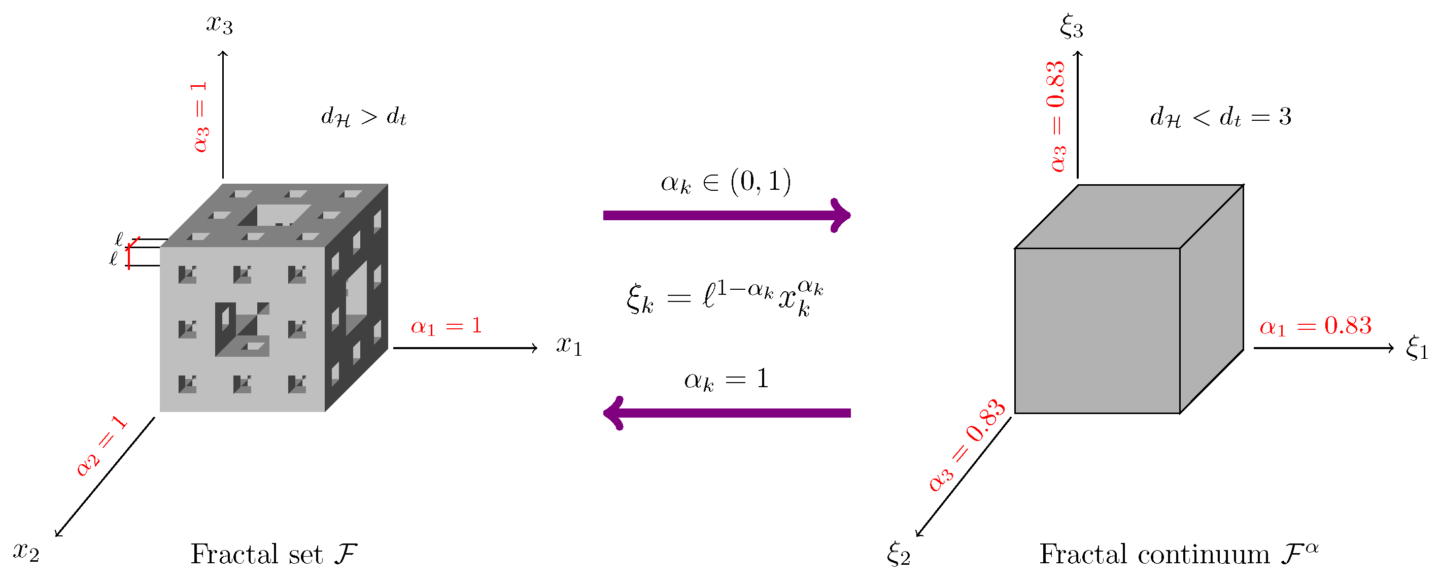
2.1. Balankin’s Approach

This fractal continuum calculus is an approach developed to describe physical phenomena occurring in natural and man-made materials, which have similar properties in a wide range of scales. Consequently, non-conventional local derivatives with fractal metrics are defined as follows [33]: a fractal continuum norm is given by $\Vert A\Vert ={\left[{\sum }_k^3{\xi }_k^{2\gamma }\right]}^{1/2\gamma }$, where $\gamma =dimC/3\le 1$, and the mapping of the integer coordinates $x_k\in E^3$ to the fractional coordinates ${\xi }_k\in {\mathcal{F}}^{\gamma }$ is defined as

$$\begin{array}{c}\hfill \zeta ={\ell }^{1-\alpha }{x}^{\alpha },\end{array}$$

(4)

where ℓ denotes the lower cutoff of fractality and $\alpha$ denotes the Hausdorff dimension in each fractional direction ${\xi }_k\in E^3$. Integer and fractal configurations are shown in Figure 1. The distance between the two points $A,B\in {\mathcal{F}}^{\gamma }$ is given by $\Delta (A,B)={\left[{\sum }_x^3{\Delta }_x^{2\gamma }\right]}^{1/2\gamma }$, where ${\Delta }_x=\Vert {\xi }_{ax}-{\xi }_{bx}\Vert$, and the fractal continuum gradient ${\nabla }^{\alpha }={\mathbf{e}}_x{\nabla }_x^{\alpha }$, where ${\mathbf{e}}_x$ are basis vectors and

$$\begin{array}{c}\hfill {\nabla }_x^{\alpha }={\alpha }^{-1}{\left(x/\ell \right)}^{1-\alpha }{\nabla }_x,\end{array}$$

(5)

which denotes the spatial fractal continuum derivative. It is easy to see that if $\alpha =1$ in Equation (5), the spatial Balankin derivative is equal to the spatial derivative in the conventional sense.

The divergence operator is expressed as ${\nabla }^{\alpha }·\overrightarrow{F}$ and, therefore, the fractal continuum Laplacian is defined as ${\Delta }^{\alpha }={\nabla }^{\alpha }·{\nabla }^{\alpha }f={\sum }_x^3{\left(c_1^{\left(x\right)}\right)}^{-2}\left[{\nabla }_x^2+{\displaystyle \frac{\gamma -\alpha }{x}}\nabla \right]$, where $c_1^{\left(x\right)}=\alpha {\ell }^{1-\alpha }{x}^{\alpha -1}$.

The temporal fractal continuum derivative defined in Balankin’s approach is introduced in Balankin and Elizarraraz [31] as

$$\begin{array}{c}\hfill {\nabla }_t^H={(t/\tau +1)}^{1-\beta }{\nabla }_t,\end{array}$$

(6)

where $\tau$ is the intrinsic time; meanwhile, $\beta$ is the intrinsic time exponent. In [34], it was derived via the following relation:

$$\begin{array}{c}\hfill \beta =dimS/n_{\gamma },\end{array}$$

(7)

where $n_{\gamma }=2dimC-dimS$ is the number of effective spatial degrees of freedom of a random walker on the studied fractal. Once again, Equation (6) is equal to the conventional partial time derivative when $\beta =1$. Here, the fractal parameter $0<\beta \le 1$ implies the fractional order with the fractal metric of any partial differential equation under study.

The derivativatives defined above can be calculated in the conventional sense, and they are employed to generalize equations and formulations of material scale invariants from conventional to fractal calculus. This methodology has been successfully utilized in different engineering applications, such as Balankin et al. [35], Balankin [36], Samayoa et al. [37,38,39] and Damián-Adame et al. [40].

2.2. Fractal Continuum Maxwell Creep Model

The conventional Maxwell model given in Equation (1) can be generalized from the integer space to fractal continuum space using Equation (6) as follows:

$$\begin{array}{c}\hfill {\displaystyle \frac{d{\epsilon }^{\beta }}{dt}}={\displaystyle \frac{1}{E}}{\displaystyle \frac{d\sigma }{dt}}+{\displaystyle \frac{\sigma }{\eta }}{\left({\displaystyle \frac{t}{\tau }}+1\right)}^{\beta -1},\end{array}$$

(8)

and by applying $\sigma ={\sigma }_0\theta \left(t\right)$ and $d\theta /dt=\delta \left(t\right)$, obtained by the definition of the Dirac delta function, we can rewrite Equation (8) as

$$\begin{array}{c}\hfill {\displaystyle \frac{d{\epsilon }^{\beta }}{dt}}={\displaystyle \frac{1}{E}}{\sigma }_0\delta \left(t\right)+{\displaystyle \frac{1}{\eta }}{\sigma }_0\theta \left(t\right){\left({\displaystyle \frac{t}{\tau }}+1\right)}^{\beta -1}.\end{array}$$

(9)

Note that Equation (9) is equal to the conventional Maxwell creep equation when the spectral and chemical dimensions are equal to $d_s/d_{ch}=1$. The general solution of Equation (9) is found when $ϵ=const$. Meanwhile, the particular solution is obtained as follows:

$$\begin{array}{c}\hfill {\epsilon }_p^{\beta }=\int \left({\displaystyle \frac{1}{E}}{\sigma }_0\delta \left(t\right)+{\displaystyle \frac{1}{\eta }}{\sigma }_0\theta \left(t\right){\left[{\displaystyle \frac{t}{\tau }}+1\right]}^{\beta -1}\right)dt,\end{array}$$

(10)

and this leads to the following expression:

$$\begin{array}{c}\hfill {\epsilon }_p^{\beta }={\sigma }_0\left[{\displaystyle \frac{1}{E}}\theta \left(t\right)+{\displaystyle \frac{1}{\eta }}\int {\left({\displaystyle \frac{t}{\tau }}+1\right)}^{\beta -1}\theta \left(t\right)dt\right].\end{array}$$

(11)

Solving the integral via Equation (11) and applying the variable change $t/\tau +1=x$ and $dt/\tau =dx$, we have

$$\begin{array}{c}\hfill {\int }_0^t{\left({\displaystyle \frac{t}{\tau }}+1\right)}^{\beta -1}dt=\tau {\int }_1^t{x}^{\beta -1}dx={\displaystyle \frac{\tau }{\beta }}\left(t^{\beta }-1\right),\end{array}$$

(12)

and substituting the above result into Equation (11) leads to

$$\begin{array}{c}\hfill {\epsilon }_p^{\beta }=C+{\sigma }_0\left[{\displaystyle \frac{1}{E}}\theta \left(t\right)+{\displaystyle \frac{\theta \left(t\right)\tau }{\eta \beta }}\left(t^{\beta }-1\right)\right].\end{array}$$

(13)

Due to $ϵ\left(t\right)={\sigma }_{0}J\left(t\right)$ and $J\left(t\right){\mid }_{t=0}=1/E$, $C={\sigma }_0\tau /\eta \beta$, finally, the fractal continuum strain creep ${ϵ}^{\beta }$ is given as

$$\begin{array}{c}\hfill {\epsilon }_p^{\beta }={\sigma }_0\left({\displaystyle \frac{\theta \left(t\right)}{E}}+{\displaystyle \frac{\theta \left(t\right)\tau t^{\beta }}{\eta \beta }}\right)=\sigma \left({\displaystyle \frac{1}{E}}+{\displaystyle \frac{\tau t^{\beta }}{\eta \beta }}\right).\end{array}$$

(14)

So, the creep compliance $J^{\beta }\left(t\right)={ϵ}^{\beta }\left(t\right)/\sigma$ is

$$\begin{array}{c}\hfill J^{\beta }\left(t\right)={\displaystyle \frac{1}{E}}+{\displaystyle \frac{\tau t^{\beta }}{\eta \beta }}.\end{array}$$

(15)

On the other hand, the relaxation modulus is obtained from Equation (8), sustituting $ϵ={ϵ}_{0}H\left(t\right)$ into it, such that

$$\begin{array}{c}\hfill E{\epsilon }_0^{\beta }{\displaystyle \frac{dH\left(t\right)}{dt}}={\displaystyle \frac{d\sigma }{dt}}+{\displaystyle \frac{E}{\eta }}{\left[{\displaystyle \frac{t}{\tau }}+1\right]}^{\beta -1}\sigma \left(t\right),\end{array}$$

(16)

and if we made the variable change $(E/\eta ){(t/\tau +1)}^{\beta -1}\sigma \left(t\right)=\alpha \left(t\right)$ and recall that $dH/dt=\delta \left(t\right)$, the general solution of Equation (16) is

$$\begin{array}{c}\hfill \sigma \left(t\right)=C{e}^{-\int \alpha \left(t\right)dt}+e^{-\int \alpha \left(t\right)dt}\int e^{\int \alpha \left(t\right)dt}E{ϵ}_0\delta \left(t\right)dt,\end{array}$$

(17)

and then integral one leads to

$$\begin{array}{c}\hfill \int \alpha \left(t\right)dt={\displaystyle \frac{E\tau }{\eta \beta }}{\left({\displaystyle \frac{t}{\tau }}+1\right)}^{\beta },\end{array}$$

(18)

and integral two leads to

$$\begin{array}{c}\hfill \int e^{{\displaystyle \frac{E\tau }{\eta \beta }}{\left({\displaystyle \frac{0}{\tau }}+1\right)}^{\beta }}E{ϵ}_0\delta \left(t\right)dt=E{ϵ}_0{e}^{{\displaystyle \frac{E\tau }{\eta \beta }}}H\left(t\right).\end{array}$$

(19)

Sustituting both integrals into Equation (17), we have

$$\begin{array}{c}\hfill \sigma \left(t\right)=\left(C+H\left(t\right)E{ϵ}_0{e}^{{\displaystyle \frac{E\tau }{\eta \beta }}}\right)e^{-{\displaystyle \frac{E\tau }{\eta \beta }}{\left({\displaystyle \frac{t}{\tau }}+1\right)}^{\beta }}.\end{array}$$

(20)

Moreover, $\sigma \left(t\right)={\epsilon }_{0}G\left(t\right)$ and $G\left(t\right){\mid }_{t=0}=E$, so $C=0$; therefore, the relaxation stress in the fractal space-time continuum is given by

$$\begin{array}{c}\hfill {\sigma }^{\beta }\left(t\right)=E{ϵ}_0{e}^{{\displaystyle \frac{E\tau }{\eta \beta }}\left[1-{\left({\displaystyle \frac{t}{\tau }}+1\right)}^{\beta }\right]}H\left(t\right).\end{array}$$

(21)

Finally, the relaxation modulus of creep $G^{\beta }\left(t\right)$ is obtained by sustituting $ϵ={ϵ}_{0}H\left(t\right)$ into the above equation, along with $G\left(t\right)=\sigma \left(t\right)/ϵ$; therefore, we have

$$\begin{array}{c}\hfill G^{\beta }\left(t\right)=E{e}^{{\displaystyle \frac{E\tau }{\eta \beta }}\left[1-{\left({\displaystyle \frac{t}{\tau }}+1\right)}^{\beta }\right]}.\end{array}$$

(22)

The effect of the varible-order $\beta$ is shown in Figure 2 for creep compliance $J^{\beta }\left(t\right)$ and the relaxation modulus $G^{\beta }\left(t\right)$.

3. Study of the Fractal Continuum Maxwell Model in Specimen Sierpinski’s Carpets Type

The objective of this section is to apply the fractal formulation developed in specimens with fractal geometry.

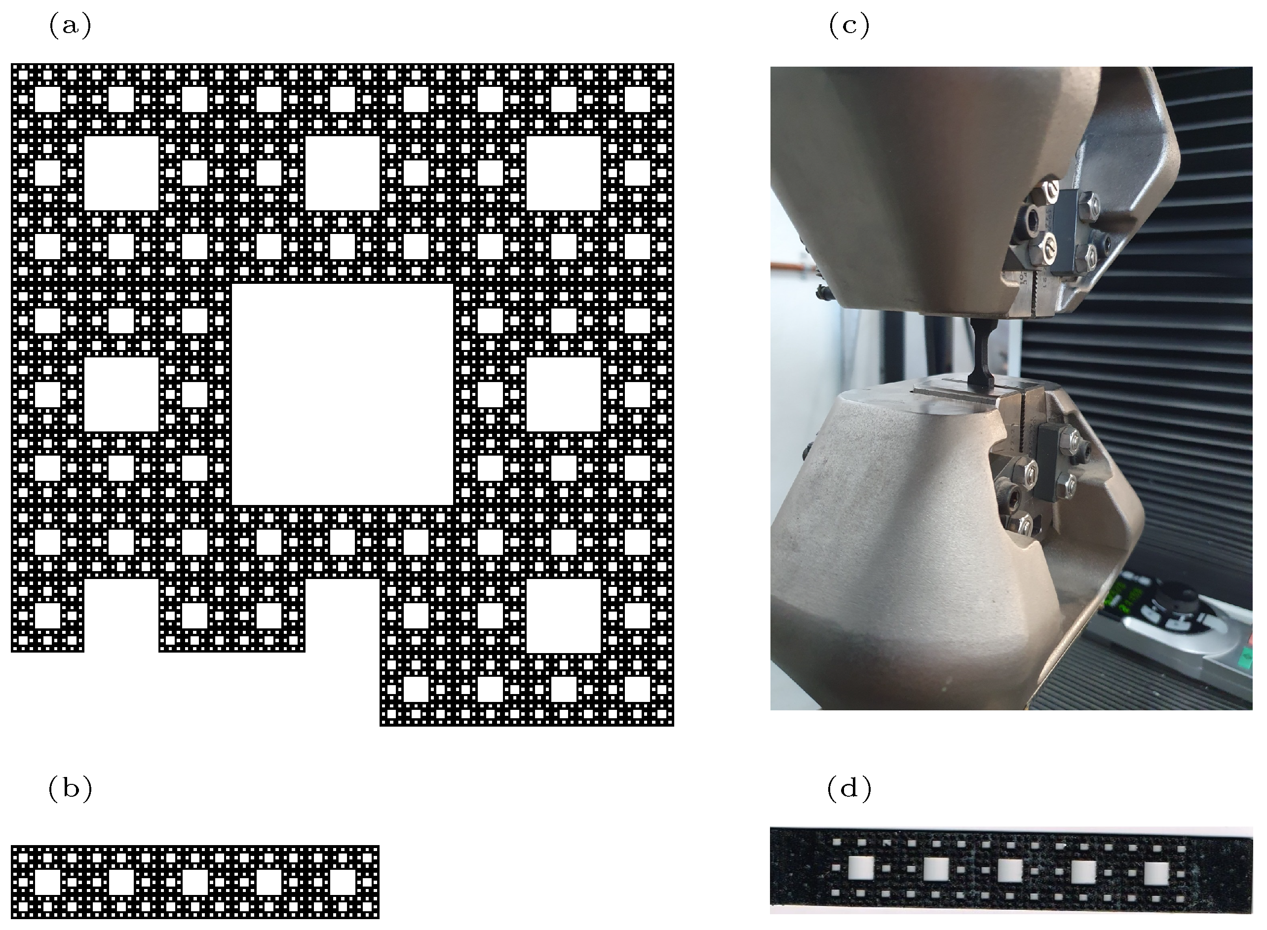
3.1. Sierpinski’s Carpets

Sierpinski carpet denoted by ${\mathcal{S}}^{\ell }$ is a classical example of a two-dimensional self-similar fractal, and it can be constructed by an iterative process from the unit square ${[0,1]}^2$. The initial square is divided into $\ell \times \ell$ sub-squares of equal size, and the interiors of $B^2$ sub-squares are eliminated. After repeating this process many times, ${\mathcal{S}}^{\ell }\in {\Re }^2$ is obtained. Its Hausdorff dimension is defined as [41]

$$\begin{array}{c}\hfill dimH={\displaystyle \frac{log\left(N{(\ell )}^2-B^2\right)}{logN(\ell )}},\end{array}$$

(23)

where $N(\ell )$ is the number of boxes covering the fractal mass with size ℓ, and $B^2$ is the number of deleted boxes of the fractal mass. Note that $\ell \times \ell$ is the size of sub-squares, which are eliminated in the k-th iteration of the corresponding Sierpinski carpet.

The chemical dimension of a Sierpinki carpet is defined by $N(L/{\ell }_{ch})\sim {(L/{\ell }_{ch})}^{dimC}$. In this scaling law, $N(L/{\ell }_{ch})$ represents the number of $dimC$-dimensional boxes of size ${\ell }_{ch}$ needed to cover the fractal according to the scale invariance principle, where ${\ell }_{ch}$ is measured with respect to the geodesic metric over the Sierpinski carpet. The Euclidean and geodesic metrics are equivalents, as shown by Cristea [42]; therefore, the chemical dimension is equal to the Hausdorff dimension.

It is well known that the density of the Sierpinski carpet vibration mode scales with frequency $\omega$ as $\Omega \left(\omega \right)\sim {\omega }^{dimS-1}$, where $dimS$ is the spectral dimension determining the scaling properties of the eigenvalues of the Laplacian defined on $S^{\xi }$. The spectral dimension of the Sierpinki carpet can be determined by [43]:

$$\begin{array}{c}\hfill dimS=2{\displaystyle \frac{log\left[N{(\ell )}^2-B^2\right]}{log\left[N{(\ell )}^2+B^2\right]}}.\end{array}$$

(24)

In Table 1, the fractal dimensional numbers for ${\mathcal{S}}^{\ell }$ used in this study are presented; meanwhile, in Figure 3, the configurations of two Sierpinski carpets are detailed.

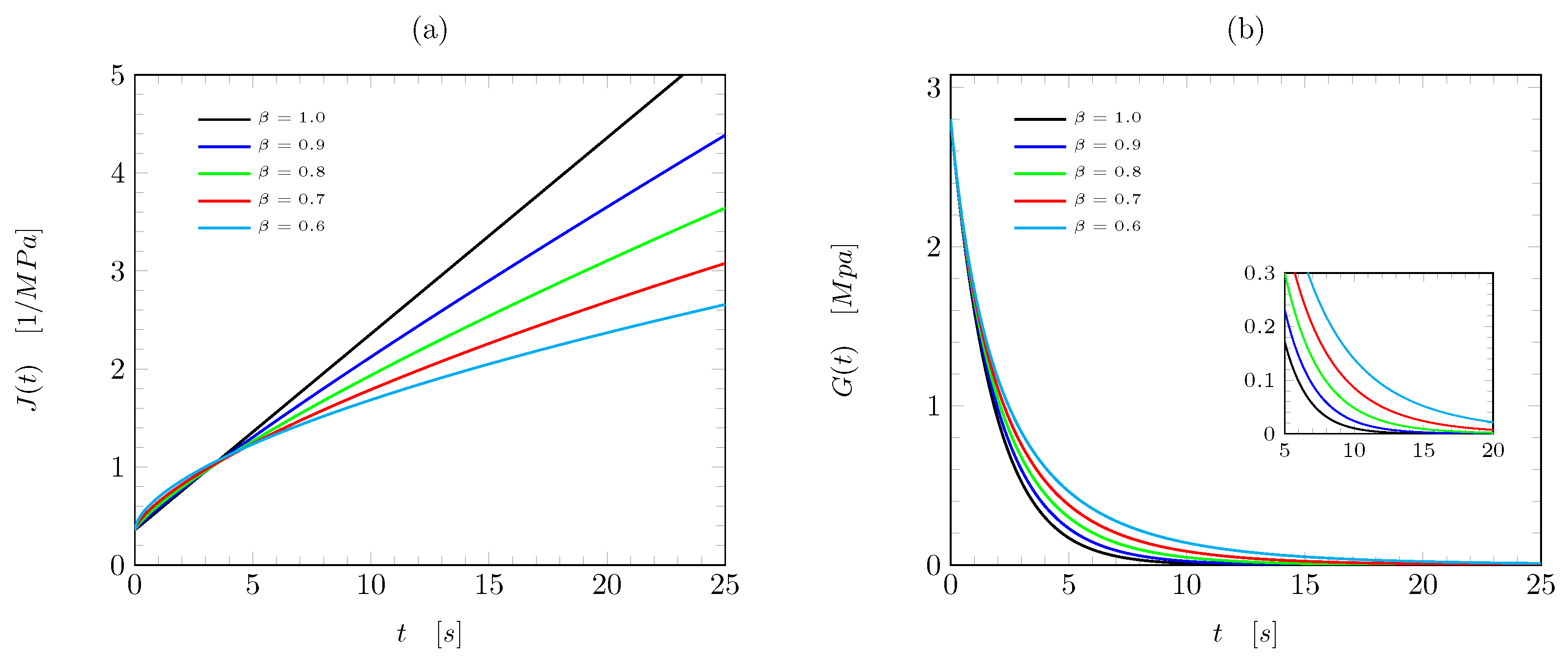
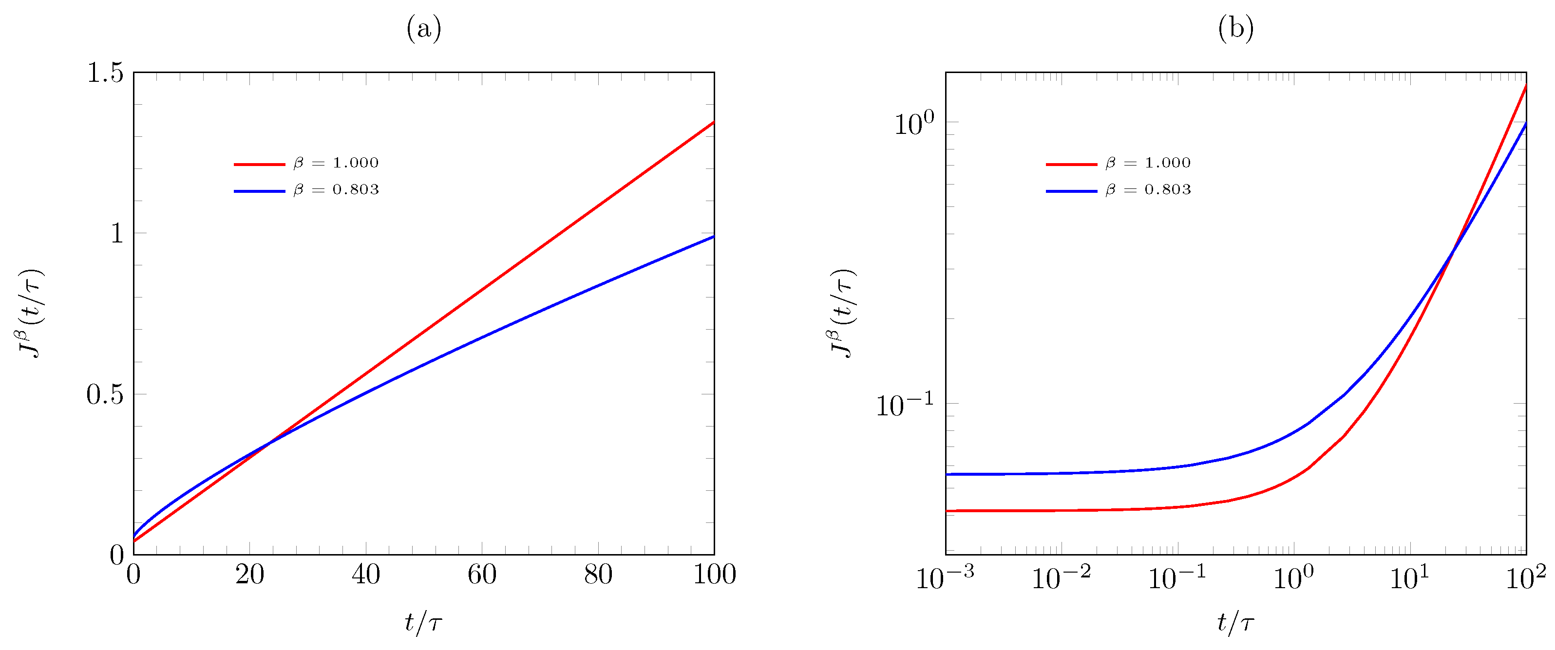
3.2. Theoretical Applications

Resione F69 flexible resin [7] samples used for the validation of the proposed model were fabricated with fractal geometry extracted from the Sierpinski carpet of the fifth iteration $i=5$, using the mechanical properties presented in

Table 2. Mechanical properties of fractal material.

Tensile Strength (MPa)	$4.87\pm 0.6$
Percent elongation at break	$175.00\pm 9.0$
Young modulus (MPa)	$23.53\pm 0.6$
Nominal strain at break	$182.00\pm 8.0$

. At least 10 samples were used in the experimental test.

All samples analyzed were rectangular cuboids of thickness $w=1\pm 0.12$ mm with length $L=100\pm 0.12$ mm along the $x_1$-axis and a height of $h=15\pm 0.12$ mm in the $x_3$-axis direction. In Figure 3b, it can be seen that the designed sample is part of the fifth iteration of the basic Sierpinski carpet, constructed with five squares; each one of them is of the third iteration. Based on the self-similarity properties, the fractal samples have the same Hausdorff dimension as the entire Sierpinski carpet.

Figure 4 and Figure 5 present the graphs of the theoretical values of creep compliance and relaxation modulus, respectively.

4. Analysis and Discussion of Results

Figure 2 shows curves for fractal continuum creep compliance with several values of $\beta$. It is a straightforward matter to see that the value of $J\left(t\right)$ is becoming lower as the fractal dimension of time scale ($\beta$) decreases; however, all fractal creep compliances in Figure 2a converge at $t=3.5$ s. Note that when $\beta =1$, the creep compliance of the fractal continuum Maxwell model reduces to standard form. Howver, Figure 2b presents the relaxation stress $G^{\beta }\prime \left(t\right)$ for $\beta =0.6,0.7,0.8,0.9,1.0$. The graph inset in Figure 2b displays a close up of the relaxation stress behavior, whose curves match with the results reported in Figure 3 from reference [15].

In Figure 4, the fractal continuum creep model prediction obtained from Equation (9) with $\beta =dimS/dimC=0.953$ (see Table 1) is presented, and it is in a very good agreement with the experimentally obtained data from the samples with the classic Sierpinski carpet structure. In addition, Figure 5 presents the fractal relaxation modulus $G^{\beta }$ for the standard and fractal versions.

In the case of the creep strain rate in the fractal continuum space-time ${ϵ}^{\beta }\prime \left(t\right)$, we found a power law behavior for the variable-order of $\beta$. The graph shown in Figure 6a was obtained by the least square method, where ${ϵ}^{\beta }\prime \left(t\right)$ depends on the beta order, such that ${ϵ}^{\beta }\prime \left(t\right)\sim t^{\beta -2}$ with a determination coefficient of $R^2=0.99$. This results are in accordance with results given in [44,45]. However, the impact of fractality is observed, which depends on $\beta$, and the slope $\beta -2$ is constant for a wide range of scales. On the other hand, the creep strain rate with respect to time for any applied stress behavior is also a power law but with the same stresses. Figure 6b shows the curves that show the behavior of ${ϵ}^{\beta }\prime \left(t\right)$ for $\beta =0.803$, where ${ϵ}^{\beta }\prime \left(t\right)\sim t^{-1/2}$ matches with the results reported by Liu et al. [46].

The obtained model has a resemblance to the results acquired in models that incorporate fractional geometry. However, our model includes the topology and fractal geometry through the different Hausdorff dimensions of th fractal material under study. Moreover, it captures material’s heterogeneity using the alpha parameter (which depends on its fractal geometry and topology) and its dynamical characteristics through the spectral dimension.

Consequently, the engineering implications of the generalized fractal continuum Maxwell creep equation that extends the standard equation to fractal manifolds are that it is able to describe the creep phenomena in viscoelastic materials that have non-classical characteristics, possess scale invariance, and cannot be described using conventional calculus. The proposed model contains the fractal parameter $\beta$, which is an additional parameter not included in preceding fractional models, where the Maxwell creep is used, which is a two-element model consisting of a linear spring element and a linear viscous dashpot element connected in series, as shown in Figure 7. This is different from the behavior of the fractal Kelvin–Voigt creep model suggested in [47], where a spring element and dashpot element are connected in parallel (see Figure 1 of Ref. [11], which adds a short review of other creep models).

It is worth noting that both the Maxwell and Kelvin–Voigt models can be described with other alternative approaches, such as the concepts of space-time radial basis function [48,49], which is a type of function used for solving partial differential equations across both time and space dimensions [50,51]. Also, the equivalent continuum method had proved to be effective when using ordinary calculus on pre-fractals [52].

5. Conclusions

A fractal generalization of the standard Maxwell creep model is obtained using Balankin’s approach.

The concept of the fractal continuum Maxwell creep solution is established, where the discontinuities in fractal domains are mapped to the continual domains in the fractal continuum space-time using the local fractional differential operators and proportionality constants given in Equations (4)–(7), such that the creep phenomena can be described for complex and heterogeneous domains. Then, the suggested model is able to predict with effectiveness the creep behavior in heterogeneous and unconventional materials where ordinary calculus is no longer valid. The complex domain can be described by a set of fractal dimensional numbers, which characterizes their topology and fractal geometry.

When the experimental data are compared with the results of the fractal model, the information obtained from different models, as well as from the one proposed here, indicates that slow continuous deformation with the fractal continuum approach is able to provide a better description of the characteristics of fractal creep with higher precision and pliability. Moroever, the fractal formulation proposed incorporates a set of fractal dimensional numbers, which makes possible a description of the phenomena under study, as given by Equations (15) and (22).

The slow continuous deformation given by Equation (9) is linked to the topology and fractal geometry of viscoelastic fractal materials with the scaling exponent $\beta \in (0,1]$, which depends on the Hausdorff dimension of the self-similar model of the viscoelastic material and its chemical dimension.

In the particular case of $\beta =1$, the fractal model suggested reduces to a normal creep Maxwell model.

References

1. Daghigh, V.; Edalati, H.; Daghigh, H.; Belk, D.M.; Nikbin, K. Time-dependent creep analysis of ultra-high-temperature functionally graded rotating disks of variable thickness. Forces Mech. 2023, 13, 100235. [Google Scholar] [CrossRef]
2. Seddighi, H.; Ghannad, M.; Loghman, A.; Zamani Nejad, M. Creep analysis of a cylinder subjected to 2D thermoelasticity loads and boundary conditions with inner heat generation source. Forces Mech. 2024, 15, 100271. [Google Scholar] [CrossRef]
3. Kumar, N.; Alen, S.; Mehrotra, P.; Yadav, S. An improved dislocation density reliant model to address the creep deformation of reduced activation ferritic martensitic steel. Forces Mech. 2022, 9, 100117. [Google Scholar] [CrossRef]
4. Hiemer, S.; Moretti, P.; Zapperi, S.; Zaiser, M. Predicting creep failure by machine learning—Which features matter? Forces Mech. 2022, 9, 100141. [Google Scholar] [CrossRef]
5. Findley, W.; Lai, J.; Onaran, K. Creep and Relaxation of Nonlinear Viscoelastic Materials: With an Introduction to Linear Viscoelasticity; Dover Civil and Mechanical Engineering: Dover, UK, 1989. [Google Scholar]
6. Farfan-Cabrera, L.; Pascual-Francisco, J. An Experimental Methodological Approach for Obtaining Viscoelastic Poisson’s Ratio of Elastomers from Creep Strain DIC-Based Measurements. Exp. Mech. 2022, 62, 287–297. [Google Scholar] [CrossRef]
7. Pascual-Francisco, J.; Susarrey-Huerta, O.; Farfan-Cabrera, L.; Flores-Hernández, R. Creep Properties of a Viscoelastic 3D Printed Sierpinski Carpet-Based Fractal. Fractal Fract. 2023, 7, 568. [Google Scholar] [CrossRef]
8. Mainardi, F. Fractional Calculus and Waves in Linear Viscoelasticity: An Introduction to Mathematical Models; World Scientific: Singapore, 2022. [Google Scholar]
9. Scott Blair, G. Analytical and Integrative Aspects of the Stress-Strain-Time Problem. J. Sci. Instrum. 1944, 21, 80. [Google Scholar] [CrossRef]
10. Zhang, Y.; Liu, X.; Yin, B.; Luo, W. A Nonlinear Fractional Viscoelastic-Plastic Creep Model of Asphalt Mixture. Polymers 2021, 13, 1278. [Google Scholar] [CrossRef]
11. Ribeiro, J.G.T.; de Castro, J.T.P.; Meggiolaro, M.A. Modeling concrete and polymer creep using fractional calculus. J. Mater. Res. Technol. 2021, 12, 1184–1193. [Google Scholar] [CrossRef]
12. Bouras, Y.; Vrcelj, Z. Fractional and fractal derivative-based creep models for concrete under constant and time-varying loading. Constr. Build. Mater. 2023, 367, 130324. [Google Scholar] [CrossRef]
13. Garra, R.; Mainardi, F.; Spada, G. A generalization of the Lomnitz logarithmic creep law via Hadamard fractional calculus. Chaos Solitons Fractals 2017, 102, 333–338. [Google Scholar] [CrossRef]
14. Giusti, A.; Colombaro, I.; Garra, R.; Garrappa, R.; Mentrelli, A. On variable-order fractional linear viscoelasticity. Fract. Calc. Appl. Anal. 2024, 27, 1564–1578. [Google Scholar] [CrossRef]
15. Cai, W.; Chen, W.; Xu, W. Characterizing the creep of viscoelastic materials by fractal derivative models. Int. J. Non-Linear Mech. 2016, 87, 58–63. [Google Scholar] [CrossRef]
16. Wang, R.; Zhuo, Z.; Zhou, H.; Liu, J. A fractal derivative constitutive model for three stages in granite creep. Results Phys. 2017, 7, 2632–2638. [Google Scholar] [CrossRef]
17. Yin, Q.; Dai, J.; Dai, G.; Gong, W.; Zhang, F.; Zhu, M. Study on Creep Behavior of Silty Clay Based on Fractal Derivative. Appl. Sci. 2022, 12, 8327. [Google Scholar] [CrossRef]
18. Chen, W. Time-space fabric underlying anomalous diffusion. Chaos Soliton Fractals 2006, 28, 923–929. [Google Scholar] [CrossRef]
19. Chen, W.; Zhang, X.; Korosak, D. Investigation on Fractional and Fractal Derivative Relaxation-Oscillation Models. Int. J. Nonlinear Sci. Numer. Simul. 2010, 11, 3–9. [Google Scholar] [CrossRef]
20. Mandelbrot, B. The Fractal Geometry of Nature; WH Freeman: New York, NY, USA, 1982. [Google Scholar]
21. Falconer, K. Fractal Geometry: Mathematical Foundations and Applications; John Wiley and Sons, Ltd.: Chichester, UK, 2014. [Google Scholar]
22. Husain, A.; Nanda, M.; Chowdary, M.; Sajid, M. Fractals: An Eclectic Survey, Part-I. Fractal Fract. 2022, 6, 89. [Google Scholar] [CrossRef]
23. Husain, A.; Nanda, M.; Chowdary, M.; Sajid, M. Fractals: An Eclectic Survey, Part-II. Fractal Fract. 2022, 6, 379. [Google Scholar] [CrossRef]
24. Balankin, A.S. Fractional space approach to studies of physical phenomena on fractals and in confined low-dimensional systems. Chaos Solitons Fractals 2020, 132, 109572. [Google Scholar] [CrossRef]
25. Patino-Ortiz, J.; Patino-Ortiz, M.; Martínez-Cruz, M.A.; Balankin, A. A Brief Survey of Paradigmatic Fractals from a Topological Perspective. Fractal Fract. 2023, 7, 597. [Google Scholar] [CrossRef]
26. Balka, R.; Buczolich, Z.; Elekes, M. A new fractal dimension: The topological Hausdorff dimension. Adv. Math. 2015, 274, 881–927. [Google Scholar] [CrossRef]
27. Balankin, A.; Patino, J.; Patino, M. Inherent features of fractal sets and key attributes of fractal models. Fractals 2022, 30, 2250082. [Google Scholar] [CrossRef]
28. Mosco, U. Invariant field metrics and dynamical scalings on fractals. Phys. Rev. Lett. 1997, 79, 4067–4070. [Google Scholar] [CrossRef]
29. Havlin, S.; Ben-Avraham, D. Diffusion in disordered media. Phi 2002, 52, 187–292. [Google Scholar] [CrossRef]
30. Balankin, A.S.; Elizarraraz, B.E. Hydrodynamics of fractal continuum flow. Phys. Rev. E 2012, 85, 025302(R). [Google Scholar] [CrossRef]
31. Balankin, A.S.; Elizarraraz, B.E. Map of fluid flow in fractal porous medium into fractal continuum flow. Phys. Rev. E 2012, 85, 056314. [Google Scholar] [CrossRef]
32. Balankin, A.S.; Elizarraraz, B.E. Reply to “Comment on ‘Hydrodynamics of fractal continuum flow’ and ‘Map of fluid flow in fractal porous medium into fractal continuum flow’”. Phys. Rev. E 2013, 88, 057002. [Google Scholar] [CrossRef]
33. Balankin, A.S. A continuum framework for mechanics of fractal materials I: From fractional space to continuum with fractal metric. Eur. Phys. J. 2015, 88, 90. [Google Scholar] [CrossRef]
34. Balankin, A.S. Effective degrees of freedom of a random walk on a fractal. Phys. Rev. E 2015, 92, 062146. [Google Scholar] [CrossRef]
35. Balankin, A.S.; Mena, B.; Patino, J.; Morales, D. Electromagnetic fields in fractal continua. Phys. Lett. A 2013, 377, 783–788. [Google Scholar] [CrossRef]
36. Balankin, A.S. A continuum framework for mechanics of fractal materials II: Elastic stress fields ahead of cracks in a fractal medium. Eur. Phys. J. 2015, 88, 91. [Google Scholar] [CrossRef]
37. Samayoa, D.; Damián, L.; Kriyvko, A. Map of bending problem for self-similar beams into fractal continuum using Euler-Bernoulli principle. Fractal Fract. 2022, 6, 230. [Google Scholar] [CrossRef]
38. Samayoa, D.; Kriyvko, A.; Velázquez, G.; Mollinedo, H. Fractal Continuum Calculus of Functions on Euler-Bernoulli Beam. Fractal Fract. 2022, 6, 552. [Google Scholar] [CrossRef]
39. Samayoa, D.; Alcántara, A.; Mollinedo, H.; Barrera-Lao, F.; Torres-SanMighel, C. Fractal Continuum Mapping Applied to Timoshenko Beams. Mathematics 2023, 11, 3492. [Google Scholar] [CrossRef]
40. Damián-Adame, L.; Gutiérrez-Torres, C.C.; Figueroa-Espinoza, B.; Barbosa-Saldaña, J.G.; Jiménez-Bernal, J.A. A Mechanical Picture of Fractal Darcy’s Law. Fractal Fract. 2023, 7, 639. [Google Scholar] [CrossRef]
41. Cristea, L.L.; Steinsky, B. Connected generalised Sierpinski carpets. Topol. Its Appl. 2010, 157, 1157–1162. [Google Scholar] [CrossRef]
42. Cristea, L. A geometric property of the Sierpiński carpet. Quaest. Math. 2005, 28, 251–262. [Google Scholar] [CrossRef]
43. Balankin, A.S. The topological Hausdorff dimension and transport properties of Sierpinski carpets. Phys. Lett. A 2017, 381, 2801–2808. [Google Scholar] [CrossRef]
44. Rieth, M. A comprising steady-state creep model for the austenitic AISI 316 L(N) steel. J. Nucl. Mater. 2007, 367–370, 915–919. [Google Scholar] [CrossRef]
45. Pineda León, E.; Samayoa Ochoa, D.; Rodríguez-Castellanos, A.; Aliabadi, M.; Avalos Gauna, E.; Olivera-Villaseñor, E. Creeping analysis with variable temperature applying the boundary element method. Eng. Anal. Bound. Elem. 2012, 36, 1715–1720. [Google Scholar] [CrossRef]
46. Liu, W.; Zhou, H.; Zhang, S.; Jiang, S.; Yang, L. A nonlinear creep model for surrounding rocks of tunnels based on kinetic energy theorem. J. Rock Mech. Geotech. Eng. 2023, 15, 363–374. [Google Scholar] [CrossRef]
47. Reyes de Luna, E.; Kryvko, A. Pascual-Francisco, J.; Hernández, I.; Samayoa, D. Generalized Kelvin–Voigt Creep Model in Fractal Space–Time. Mathematics 2024, 12, 3099. [Google Scholar] [CrossRef]
48. Myers, D.; De Iaco, S.; Posa, D.; De Cesare, L. Space-time radial basis functions. Comput. Math. Appl. 2002, 43, 539–549. [Google Scholar] [CrossRef]
49. Hamaidi, M.; Naji, A.; Charafi, A. Space–time localized radial basis function collocation method for solving parabolic and hyperbolic equations. Eng. Anal. Bound. Elem. 2016, 67, 152–163. [Google Scholar] [CrossRef]
50. Noorizadegan, A.; Chen, C.S.; Young, D.; Chen, C. Effective condition number for the selection of the RBF shape parameter with the fictitious point method. Appl. Numer. Math. 2022, 178, 280–295. [Google Scholar] [CrossRef]
51. Amir Noorizadegan, D.L.Y.; Chen, C.S. Space–time method for analyzing transient heat conduction in functionally graded materials. Numer. Heat Transf. Part B Fundam. 2024, 85, 828–841. [Google Scholar] [CrossRef]
52. Davey, K.; Rasgado, M. Analytical solutions for vibrating fractal composite rods and beams. Appl. Math. Model. 2011, 35, 1194–1209. [Google Scholar] [CrossRef]
Figure 1. A geometrical interpretation of fractal continuum calculus using the classical Menger sponge.
Axioms 14 00033 g001
Figure 2. Predictions of fractal creep compliance for several beta values ( E = 2.8 , η = 5 ) for (a) creep modulus, and (b) relaxation compliance.
Axioms 14 00033 g002
Figure 3. Sample with fractal geometry similar to the Sierpinski carpet S : (a) fifth iteration for = 1 / 3 , (b) self-similar part of the Sierpinski carpet with five squares of third iteration, (c) the tensile test on a dog bone sample of the constituent material, and (d) the constituent material with the fractal domain.
Axioms 14 00033 g003
Figure 4. Dimensionless fractal creep compliance J β ( t / τ ) as a function of t / τ for the Maxwell model in a specimen Sierpinski carpet type with β = 0.803 and comparison with conventional creep compliance ( β = 1 ) for (a) short times, and (b) log-log plot.
Axioms 14 00033 g004
Figure 5. The dimensionless relaxation modulus in the fractal space-time continuum for the Maxwell model in the speciment Sierpinski carpet type with β = 0.803 and β = 1 for (a) short times, and (b) semi-log plot.
Axioms 14 00033 g005
Figure 6. The creep strain rate (a) as a function of the order of fractal dimension of time scale for several values of time, as well as (b) as an applied stress function for β = 0.803 .
Axioms 14 00033 g006
Figure 7. A geometric representation of the Maxwell model.
Axioms 14 00033 g007