Round-Off Error Suppression by Statistical Averaging

Abstract

Regarding round-off errors as random is often a necessary simplification to describe their behavior. Assuming, in addition, the symmetry of their distributions, we show that one can, in unstable (ill-conditioned) computer calculations, suppress their effect by statistical averaging. For this, one slightly perturbs the argument of $f\left(x_0\right)$ many times and averages the resulting function values. In this text, we forward arguments to support the assumed properties of round-off errors and critically evaluate the validity of the averaging approach in several numerical experiments.

1. Introduction

If a measurement can be regarded as an unbiased estimation of some observable, then, by definition, one can expect (in terms of probability) the mean of several measurements to be closer to the true value than what is given by a single measurement. This simple idea has many practical applications, but, surprisingly, no such idea can be found in the literature with respect to round-off errors (often thought of as random). Here, we elaborate on this idea, although the main concept is elementary and may intuitively be seen as valid. Therefore, we focus mostly on technical aspects and arguments to show its mechanism in more detail. The commonly used normal distribution, where individual measurements are assumed to have uncorrelated errors, leads to

$${\sigma }_N\left(\mu \right)={\displaystyle \frac{{\sigma }_{\mathrm{rf}}}{\sqrt{N}}},$$

(1)

where ${\sigma }_N\left(\mu \right)$ is the error with which we estimate the mean, ${\sigma }_{\mathrm{rf}}$ is the standard deviation of the probability distribution with the mean $\mu$ from which the sample originates and N is the number of measurements. As can be readily seen, the precision increases with repeated measurements as $1/\sqrt{N}$.

We have already covered many aspects of this method in [1]; however, the primary focus there was on numerical differentiation. Here, we aim to adopt a more general approach whose scope is numerically unstable problems in general, which are usually (but not necessarily) ill conditioned (the instability of a numerical computation can result not only from the underlying ill-conditioned mathematical problem but also from an inappropriate implementation of the solution (see Section 3.1)) in the mathematical sense, too. Also, we want to examine new possible dependencies not covered until now, namely, the dependence of the results on the programming language, processor architecture and operating system.

One needs to understand what the method is suited for and what it is not. First of all, we regard our result primarily as a theoretical message, which was not so clearly stated until now: namely, one can, routinely and without some specific requirements, go beyond the usual round-off error precision. From the practical point of view, this, however, applies mostly to situations where no other means (such as arbitrary-precision software) for increasing the precision are available in circumstances where the increase in the precision is of uttermost importance. This may correspond to the evaluation of a black-box function in a fixed number format environment, like when using compiled libraries or when obtaining function values from a server where the function-evaluation process is hidden from the client. It may also possibly apply to situations where re-programming (let us say in arbitrary-precision software) is possible but very costly. The obvious disadvantage is the time consumption (see Equation (6)), together with the fact that a precision increase is typically limited to a few orders of magnitude (in absolute errors).

The extent of numerical problems we are aiming at is very broad: basically any unstable numerical computation. What generally applies to this domain is that round-off errors are considered random. This point of view is very common and found in many texts; see, e.g., [2,3,4,5]. What distinguishes us from these authors is the way we use the randomness assumption: the cited texts apply it to stable numerical problems, in which the control of the error is important, and theoretically derive confidence intervals for the results. We, on the contrary, analyze unstable computations, where we let the computer actually perform error propagation in the perturbed-argument scenario with subsequent outcome averaging. Our theoretical concern is only to show that the averaging is justified, our aim being less ambitious: support the claim that the error is generally reduced without precisely quantifying by how much (as numerical experiments show, this does depend on the problem and cannot be reliably quantified in the “black-box” scenario).

In Section 2, we carry out a theoretical analysis of the approach that we propose, and in Section 3, numerical experiments are presented.

2. Theoretical Analysis

2.1. Method Principle

The methods that implement the statistical averaging-out of round-off errors in the evaluation of $f\left(x_0\right)$ may differ in their details; here, we adopt a simple linear first-order estimator in a symmetric setting, as is explained below. In what follows, ${\alpha }_{\mathrm{fl}}$ indicates the floating-point representation of the number $\alpha$, and $x_i$ is assumed to be a machine number. We also assume that round-off errors induce important fluctuations in the function value $f_{\mathrm{fl}}\left(x\right)$ for small perturbations of its argument $x_0$ and that these fluctuations are symmetrical and significantly greater (this requirement determines our scope to be unstable numerical computations) than the function value changes. We proceed as follows:

• We generate N random numbers ${\left\{x_i\right\}}_{i=1}^N$ in a small interval around $x_0$, $x_i\in I\equiv \left(x_0-h,x_0+h\right)$, $h\ll 1$, and we assume that, in this small interval, f can be very well approximated by a linear function. Numbers $x_i$ are generated from a distribution that is symmetric with respect to $x_0$; in our case, we use a uniform distribution on the interval I.
• We evaluate computer-estimated function values ${\left\{f_{\mathrm{fl}}^i\right\}}_{i=1}^N$, $f_{\mathrm{fl}}^i\equiv f_{\mathrm{fl}}\left(x_i\right)$, which differ from the true function values by round-off errors, $f_{\mathrm{fl}}^i=f^i+{\delta }_i$.
• We estimate the value of $f\left(x_0\right)$ by computing the average:

  $$f\left(x_0\right)\approx {\displaystyle \frac{1}{N}}\sum _{i=1}^N{f}_{\mathrm{fl}}^i\equiv f_{\mathrm{AV}}\left(x_0\right).$$
  This can be interpreted as a linear regression $R\left(x\right)$ of the set ${\left\{\left(x_i,f_{\mathrm{fl}}^i\right)\right\}}_{i=1}^N$, which we understand as a simple estimator of the first order (first meaning linear). Because of the assumptions (linearity, symmetry), one arrives, in the large-N limit, at $R\left(x_0\right)=\overline{f_{\mathrm{fl}}^i}$; i.e., one can estimate $f\left(x_0\right)\approx R\left(x_0\right)$ just by averaging the function values.

To unravel the method principle, one simply writes down the expression with error terms:

$$\begin{array}{cc}\hfill {\displaystyle \frac{1}{N}}\sum _{i=1}^N{f}_{\mathrm{fl}}^i& ={\displaystyle \frac{1}{N}}\sum _{i=1}^N\left(f^i+{\delta }_i\right)={\displaystyle \frac{1}{N}}\sum _{i=1}^N\left(f^0+{\Delta }_{i}f+{\delta }_i\right)\hfill \\ \hfill & =f\left(x_0\right)+{\displaystyle \frac{1}{N}}\sum _{i=1}^N{\Delta }_{i}f+{\displaystyle \frac{1}{N}}\sum _{i=1}^N{\delta }_i,\hfill \end{array}$$

where ${\Delta }_{i}f$ denotes the change in the (true) function value, and ${\Delta }_{i}f=f^i-f^0$. If the round-off errors ${\delta }_i$ have a symmetric distribution (we address this question later), then the error estimate for $N\to \infty$ becomes

$$\begin{array}{cc}\hfill E_A& ={\left|f\left(x_0\right)-{\displaystyle \frac{1}{N}}\sum _{i=1}^N{f}_{\mathrm{fl}}^i\right|}_{N\to \infty }={\left|{\displaystyle \frac{1}{N}}\sum _{i=1}^N{\Delta }_{i}f+{\displaystyle \frac{1}{N}}\sum _{i=1}^N{\delta }_i\right|}_{N\to \infty }\hfill \\ \hfill & ={\left|{\displaystyle \frac{1}{N}}\sum _{i=1}^N{\Delta }_{i}f\right|}_{N\to \infty },\hfill \end{array}$$

which is to be compared with a single estimation of the function value

$$E_S=\left|f^0-f_{\mathrm{fl}}^0\right|=\left|{\delta }_0\right|.$$

If f was exactly linear, then in the $N\to \infty$ limit for a symmetric $x_i$ distribution, one has $\left({\sum }_{i=1}^N{\Delta }_{i}f\right)/N=0$; i.e., the average-based estimate is better than the single estimation $E_A<E_S$. For a realistic scenario where f is not exactly linear, one could make additional estimates, quantify the deviation and see how it propagates. We propose a simple one, with a bounded quadratic term and assuming, without loss of generality, $x_0=0$. One has

$$f\left(x\right)=a+bx+c{x}^2,c\ll {\displaystyle \frac{1}{h}}.$$

(2)

Keeping all of the above-mentioned assumptions, averaging leads to

$$\begin{array}{cc}\hfill {\left({\displaystyle \frac{1}{N}}\sum _{i=1}^N{\Delta }_{i}f\right)}_{N\to \infty }& ={\left({\displaystyle \frac{b}{N}}\sum _{i=1}^N{x}_i\right)}_{N\to \infty }+{\left({\displaystyle \frac{c}{N}}\sum _{i=1}^N{x}_i^2\right)}_{N\to \infty }\hfill \\ \hfill & \ll 0+{\left({\displaystyle \frac{1}{hN}}N{h}^2\right)}_{N\to \infty }=h.\hfill \end{array}$$

If the total variation $\Delta f$ in f on I does not exceed h by orders of magnitude, $\Delta f\sim h$, then $E_A<E_S$, because the variation $\Delta f$ is supposed to be significantly smaller than a typical ${\delta }_i$ (of which ${\delta }_0$ is a representative):

$$E_A={\left|{\displaystyle \frac{1}{N}}\sum _{i=1}^N{\Delta }_{i}f\right|}_{N\to \infty }<h\sim \Delta f<\overline{\left|{\delta }_i\right|}\sim \left|{\delta }_0\right|=E_S.$$

As is clear from this last example, even if the round-off errors were fully symmetric, systematic shifts (which do not average) are present in our method. There are, however, reasons to believe that these shifts are, for well-behaved functions, small with respect to round-off errors.

One can think of many alternatives for round-off error averaging. One could, for example, use a quadratic or even a higher-order regression. Alternatively, one could randomly generate m points in I, with m being a small integer, and then construct a polynomial $P_{m-1}\left(x\right)$ that interpolates them. Repeating this many times, one could average the values of these polynomials at $x_0$: $f\left(x_0\right)\approx {\displaystyle \frac{1}{N}}{\sum }_{i=1}^N{P}_{m-1}^i\left(x_0\right).$ We have tried this approach, and it did not improve our results. In fact, all of these higher-order methods are computationally more complicated, which can further increase round-off errors.

Finally, one may ask about the implications of the method for the backward error (BE) analysis. The method as constructed deals with the forward error (FE) $|f_{\mathrm{fl}}\left(x_0\right)-f\left(x_0\right)|$ and shows that it can be improved by replacing $f_{\mathrm{fl}}\left(x_0\right)\to f_{\mathrm{AV}}\left(x_0\right)$. It is a constructive approach that has a straightforward interpretation in terms of an increase in precision. The approach itself departs from simple definitions of forward/backward errors because it uses the propagation of modified arguments by the approximation $f_{\mathrm{fl}}$ of the true function f. A strict analogy applied to BE analysis would consist of perturbing the output $f_{\mathrm{fl}}\left(x_0\right)$ and studying the set of values $x^i\equiv f^{-1}\left(y^i\right)$, $y^i=f_{\mathrm{fl}}\left(x_0\right)+{ϵ}_i$ as mapped by the inverse of the exact function. The interpretation of such a procedure is unclear, and therefore, we do not see a direct connection between our approach and the BE analysis.

2.2. Symmetry Properties of Error Propagation

For the method to work, it is important that round-off errors, if interpreted as random, have a distribution with some degree of symmetry.

2.2.1. Round-Off Error Models

Simple Model

Starting with a simple unrealistic model, we assume that the computations are not deterministic, but, when repeatedly executed with the same arguments, they gain random errors and lead to different results. We also assume that the errors are not generated during elementary processor operations (which are exact), but between them: an output of the nth operation $o^{\left[n\right]}=i_1^{\left[n\right]}★i_2^{\left[n\right]},★\in \left\{+,-,\times ,÷\right\}$ acquires, before becoming the input of the following operation, a random error $i^{[n+1]}=o^{\left[n\right]}+{\delta }^{\left[n\right]}$. Denoting a machine number as a true value with error, $x={\mu }_x+{\delta }_x$, we have

$$\begin{array}{cc}\hfill x\pm y& =\left({\mu }_x\pm {\mu }_y\right)+\left[{\delta }_x\pm {\delta }_y\right],\hfill \end{array}$$

(3)

$$\begin{array}{cc}\hfill xy& ={\mu }_x{\mu }_y+\left[{\mu }_x{\delta }_y+{\mu }_y{\delta }_x+{\delta }_x{\delta }_y\right].\hfill \end{array}$$

(4)

If ${\delta }_x$ and ${\delta }_y$ originate from symmetric probability distributions, $\varrho \left(\delta \right)=\varrho \left(-\delta \right)$, and are uncorrelated, then the error distribution of the result (square brackets) is also symmetric. This follows from the fact that addition, mutual multiplication and multiplication by a constant preserve the symmetry.

This is no longer the case for division (an incorrect statement was for the division, in this regard, given in [1]; understood as a fraction ${\displaystyle \frac{a}{b}}=a\times {\displaystyle \frac{1}{b}}$, one sees that the asymmetry is generated by the second term (denominator)) and possibly other floating-point instructions that some processor architectures implement (such as the square-root “fsqrt” or sine “fsin”). As is clear from our approach, we focus on the impact of a small perturbation of arguments on the round-off error of the result. If the perturbation $\epsilon$ is small, we can assume that, on the interval $\left(x_0-\epsilon ,x_0+\epsilon \right)$, a linear approximation of the instruction ★ is valid. Since a random variable with a distribution symmetric around the mean transformed by a linear function yields a variable with a mean-symmetric distribution too, we achieve the propagation of the error symmetry, at least in this approximation.

As a consequence, symmetric error distributions are propagated, keeping the symmetry up to the final result. Generating many results and averaging them makes errors statistically cancel. In addition to the fact that the symmetry conservation is, for some operations, only approximate, other pitfalls are present, too. For example, one can mention large (round-off) errors in the input (so that the straight-line approximation is not valid) or correlated numbers, e.g., the evaluation of $f\left(x\right)=x^2$ in the proximity of zero, which leads to asymmetric errors in the result since the latter cannot reach negative values.

More Realistic Model

Still keeping the assumption about the randomness of round-off errors, in a more realistic approach, we need to take into account that their sources are the elementary processor operations. Since error averaging is of interest to us, we are concerned, as before, with the behavior regarding error-symmetry propagation. This is a known and non-trivial issue referred to as “bias” and does depend on the rounding strategy. Clearly, simple rounding (the rounding of the last mantissa digit is meant here) rules, such as “rounding half up”, are biased for all positional numeral systems with an even base, where the bias increases for a decreasing radix (in this sense, the binary system is the worst [3]). The argument here is a deliberate human effort in designing the processor architecture: the rounding rules on all modern computers are purposely made such that they have zero bias (e.g., “round to nearest, ties to even”; see Section 4.3 of [6]), which, by definition, means that the “error production” toward higher and smaller numbers is symmetrical.

In summary, an (approximate) error-symmetry conservation of (ideal) mathematical operations, together with symmetric error production in non-ideal processor instructions, is a combination that (approximately) conserves the symmetry of the error distributions and propagates it until the final result. An (approximately) symmetric error distribution of the result errors implies that its mean value is (close to) zero; i.e., averaging is an effective tool for removing round-off errors.

Realistic Model

Computer calculations are deterministic, and therefore, we need to perturb the argument of the function to mimic the above-assumed random character of round-off errors. This raises questions about the proper size $\epsilon$ of the perturbation. A very small (a few last mantissa bits) $\epsilon$ is not suitable because it might lead to important precision losses in the computation of $R\left(x_0\right)$. An optimal step (i.e., $\epsilon$) is expected to be significantly bigger than ${ϵ}_M\times 2^E$, where ${ϵ}_M$ is the machine epsilon and E the exponent, yet significantly smaller than the typical length by which the function varies (or better, strongly deviates from its linear approximation). A numerical test for the differentiation of common elementary functions performed with double-precision variables indeed indicates [1] a typical optimal value of $\epsilon \approx {10}^{-6}\gg {10}^{-16}\approx {ϵ}_M{|}_{E=0}$. For such functions (constant function excluded), it is reasonable to assume that, for evaluations at points far away from each other (measured in units ${ϵ}_M\times 2^E$), the round-off errors are uncorrelated. The use of function values with arguments different from $x_0$ certainly introduces some bias, i.e., a discretization error, which cannot be removed by averaging, but we have forwarded arguments as to why we expect this effect to be small.

Let us summarize the main assumptions that we use in our argumentation:

• The local absolute errors ${\sigma }_i$ can be thought of as random, described by symmetric probability distributions with a zero mean.
• The round-off errors are uncorrelated for evaluations of the function value at two different points.

2.2.2. Additional Arguments

A fully rigorous argument in favor of the averaging method can be made using only one simple assumption. Let us consider a set of function value estimates $f_{\mathrm{fl}}^i$ and assume that they are fully dominated by round-off errors (and not function value changes) so that we have no a priori way to assess which estimate is more precise than others (i.e., the information content is considered equal for all estimates). If we interpret $f_{\mathrm{fl}}^i$ as measurements with random errors described by a probability distribution, then, in terms of probability, it is always (non-strictly) better to estimate the true value of $f^0$ by taking the average of the numbers, $\overline{f}=\left({\sum }_{i=1}^N{f}_{\mathrm{fl}}^i\right)/N$, than to estimate it by picking one $f_{\mathrm{fl}}^0$ (a single evaluation of the function value directly at $x_0$). In other words, the mean (squared) distance $\Delta (x_1,x_2)\in \left\{\left|x_1-x_2\right|,{\left(x_1-x_2\right)}^2\right\}$ of a single estimation of the true value $f^0$ is always (non-strictly) greater than that of the mean $\overline{f}$:

$$\Delta (\overline{f},f_0)\le {\int }_{-\infty }^{\infty }\Delta (f,f_0)\varrho \left(f\right)df=E\left[\Delta (f,f_0)\right],$$

(5)

where E represents the expected value, and $\varrho \left(f\right)$ is an (arbitrary) probability distribution that describes $f^i$ values. This follows from the non-specific, purely mathematical properties of probability distributions; more details can be found in Appendix A (or Section 3.2 of [1]).

Except for the statement in the previous paragraph, our arguments are heuristic. Yet, any honest consideration of the problem of the round-off error propagation in realistic computer computations (that go beyond a single matrix inversion or a small number of processor instructions, or possibly some very specific calculation) has to come to the conclusion that the strict mathematical treatment (strict error bounds can be derived (very easily, if they are allowed to be arbitrarily large), and here, we mean equalities; we, of course, do not imply that the search for the best bounds is not valuable) of this topic from first principles (the arithmetic of computer registers) is, without additional assumptions, far too complex. Authors, with the aim of providing some rigorous mathematical statements, often introduce various strong assumptions (usually about the randomness and its type or the existence of derivatives), which are nothing else but heuristic, too. We prefer not to play this game, since it adds nothing to the exactness of results with respect to the first principles (but it makes the paper look more serious). Yet, we might provide some additional heuristic arguments in favor of our approach.

One of them is the central limit theorem, often mentioned in texts related to round-off errors if they are treated in a probabilistic manner. Computations typically contain many additions and, supposing that the errors related to the added values can be considered uncorrelated, the probability distribution of the result tends to the Gaussian distribution, whatever the distributions of the individual summands. The Gaussian distribution is, of course, symmetric with respect to its mean, and averaging the error annihilates it.

In a realistic computation, the perfect symmetry of the numerical error distribution cannot be expected. Yet, even for distorted, non-symmetric distributions, the estimation of the true value from the average is a better option compared to what provides a single evaluation (see the “rigorous argument” paragraph). A numerical test was also performed in Section 4.1 of [1] with respect to this issue. There, the central difference formula was used to estimate the derivatives of $sin\left(x\right)$, $exp\left(x\right)$ and $ln\left(x\right)$ at $x=1,\pi$ and $1/2$, respectively. The mean discretization parameter h was chosen to be large, $h_0={10}^{-5}$, and the produced distributions were asymmetric and, as expected for large h, shifted (not centered around the true value of the derivative). Nevertheless, the mean of each distribution was close to the true value of the central difference, which means that, even for such distorted distributions, the round-off errors average to a large extent.

2.2.3. Previous Tests and Performance

In previous numerical tests (Section 4.1 of [1]), it has been demonstrated that the expected features of our approach are manifested and that we are right in understanding how the method works. The studied distributions were highly symmetrical (the asymmetry of the charts in Figure 2 of [1] is expected due to the large bias originating from the discretization error (made large by purpose); for the highest precision, the discretization parameter needs to be small (Figure 1 of [1])), and the shrinking of the error with increasing statistics (or time t, Figure 3 of [1]) is as expected from (1):

$$\sigma \left(t\right)={\sigma }_0+{\sigma }_1/\sqrt{N}={\sigma }_0+{\sigma }_1/\sqrt{\alpha t}.$$

(6)

Here, ${\sigma }_0$ is the highest possible precision, which cannot be improved by averaging (a systematic bias such as an asymmetry of the distribution or a discretization error); ${\sigma }_1$ is the typical precision provided by a single estimation; and $\alpha$ is some proportionality constant.

3. Numerical Experiments

The numerical investigation of the averaging approach can be performed in a large number of directions. One could study the dependence of the results on the size of the perturbation h, on the precision order k of the estimator, on the function f and its test point $x_0$, on the statistics N or on the processor architecture and the programming language (and others). We applied our approach to the numerical differentiation in [1], where the dependencies on $\epsilon$, k, $f\left(x_0\right)$ and N were studied, and we consider them covered. We, therefore, study the two remaining; plus, we test the behavior of the approach for functions with more parameters (which can be perturbed independently). In what follows, we investigate the following:

• The evaluation of a function of a single variable;
• A matrix inversion in the context of trigonometric interpolation;
• The evaluation of higher derivatives of a function.

In all cases, the numerical evaluation is (purposely made) unstable so as to make sense of the averaging procedure. The argument perturbations $x_i$ are generated as random numbers with a uniform distribution from the interval $\left(x_0-h,x_0+h\right)$, where h is chosen in the form $h\left(n\right)={10}^{-n}$, $n\in \mathbb{N}$, such that it gives the best results. This means that we evaluate $f\left(x_0\right)$ using the averaging procedure for various $h\left(n\right)$, $n=1,\dots ,16$, and choose the best, which we then compare to the outcome of the single evaluation of $f\left(x_0\right)$. All variables are double precision.

The tested architectures are as follows:

• x86:

  –

  Linux: 8xIntel Core i7-4770 3.40 GHz;

  –

  Windows: Intel(R) Core(TM) i7-6700HQ CPU @ 2.60 GHz 2.60 GHz;

• ARM: Octa-core: 2×2.2 GHz Cortex-A78 and 6×2.0 GHz Cortex-A55.

The tested programming languages are as follows:

• Java (openjdk 11.0.9);
• C/C++

  –

  Linux: gcc 7.5.0;

  –

  Windows: g++ (MinGW.org GCC-6.3.0-1) 6.3.0;

• Python (2.7.17);
• JavaScript (1.5);
• MATLAB (online, version R2024a, August 2024).

Three operating systems were used:

• Linux Open SUSE Leap 15.1, kernel 4.12.14-lp151.28.91-default;
• Android 13, 5.10.186-android12, Motorola Moto G54 Power;
• Windows 10 Pro.

From these, the tested combinations (Cx) are shown in

Table 1. Tested environments.

Combination	Processor	Programming Language	Operating System
C1	x86	Java	Linux
C2	x86	C/C++	Linux
C3	x86	Python	Linux
C4	x86	JavaScript	Linux
C5	ARM	JavaScript	Android
C6	x86	C/C++	Windows
C7	x86	JavaScript	Windows
C8	(online)	MATLAB	(online)

. When running JavaScript, the Chrome web browser was used in all cases.

For the averaging procedure, we used the Kahan summation algorithm [7] to have a numerically stable computation of arithmetic means.

3.1. Simple Function

We present two examples of the averaging method applied to the evaluation of a real function of one real variable.

3.1.1. First Example

Inspired by [8], we investigate the function

$$f\left(x\right)=r_{13}\left(x\right),r_n\left(x\right)=x{r}_{n-1}\left(x\right)-{\displaystyle \frac{1}{n}},r_0=ln\left(x\right)-ln\left(x-1\right)$$

(7)

at $x_0=10$. The implemented recurrent definition (7) is numerically unstable, although the alternative expression

$$r_n\left(x\right)={\int }_0^1{\displaystyle \frac{t^n}{x-t}}dt$$

implies that the mathematical dependence is not ill conditioned. Actually, a stable evaluation on a computer is also possible, e.g., using a numerical integration method. For averaging, we use $N={10}^6$ and determine the optimal step to be $h={10}^{-4}$. The results are shown in

Table 2. The precision of the evaluation of $r_{13}\left(10\right)$, Equation (7), by the averaging method compared to the direct evaluation for different computing environments (Table 1). Despite the large statistics for randomly generated $\left\{x_i\right\}$, the results have large fluctuations and cannot be reproduced exactly.

	$\mathit{f}\left(\mathit{x}\right)={\mathit{r}}_{13}\left(\mathit{x}\right)$, ${\mathit{x}}_0=10$, $\mathit{f}\left({\mathit{x}}_0\right)=0.0078785198760532617\dots$, $\mathit{h}={10}^{-4}$
	${▵}_{\mathbf{AV}}=\left|{\mathit{f}}_{\mathbf{AV}}\left({\mathit{x}}_{\mathbf{0}}\right)-\mathit{f}\left({\mathit{x}}_{\mathbf{0}}\right)\right|$	${▵}_{\mathbf{fl}}=\left|{\mathit{f}}_{\mathbf{fl}}\left({\mathit{x}}_{\mathbf{0}}\right)-\mathit{f}\left({\mathit{x}}_{\mathbf{0}}\right)\right|$	${▵}_{\mathbf{fl}}/{▵}_{\mathbf{AV}}$
C1	≈$9.2\times {10}^{-7}$	≈$3.6\times {10}^{-4}$	≈390
C2	≈$2.8\times {10}^{-6}$	≈$3.6\times {10}^{-4}$	≈130
C3	≈$3.5\times {10}^{-6}$	≈$3.6\times {10}^{-4}$	≈100
C4	≈$3.6\times {10}^{-6}$	≈$3.6\times {10}^{-4}$	≈100
C5	≈$6.3\times {10}^{-6}$	≈$3.6\times {10}^{-4}$	≈60
C6	≈$7.6\times {10}^{-6}$	≈$3.6\times {10}^{-4}$	≈50
C7	≈$1.1\times {10}^{-6}$	≈$3.6\times {10}^{-4}$	≈330
C8	≈$1.6\times {10}^{-6}$	≈$3.6\times {10}^{-4}$	≈220

. We see an enhancement of the precision by orders of magnitude. Although the numbers differ in various rows, the difference seems to be mainly due to statistical fluctuations (random $x_i$ generation). This can be seen by looking at the value from the single evaluation (at $x_0=10$) where differences are small: all Linux and ARM calculations agree that $f_{\mathrm{fl}}^{\mathrm{L}}\left(x_0\right)=0.008235200679887617$, although Windows scenarios C6 and C7 give a quite different value: $f_{\mathrm{fl}}^{\mathrm{W}}\left(x_0\right)=0.0082350165617707458$. Still, the difference $\left|f_{\mathrm{fl}}^{\mathrm{L}}\left(x_0\right)-f_{\mathrm{fl}}^{\mathrm{W}}\left(x_0\right)\right|\approx 1.8\times {10}^{-7}$ is significantly smaller than the error produced by the single evaluation, $\approx 3.6\times {10}^{-4}$. These large fluctuations at such large statistics are somewhat surprising; nevertheless, in any scenario, the precision increase is significant and exceeds one order of magnitude.

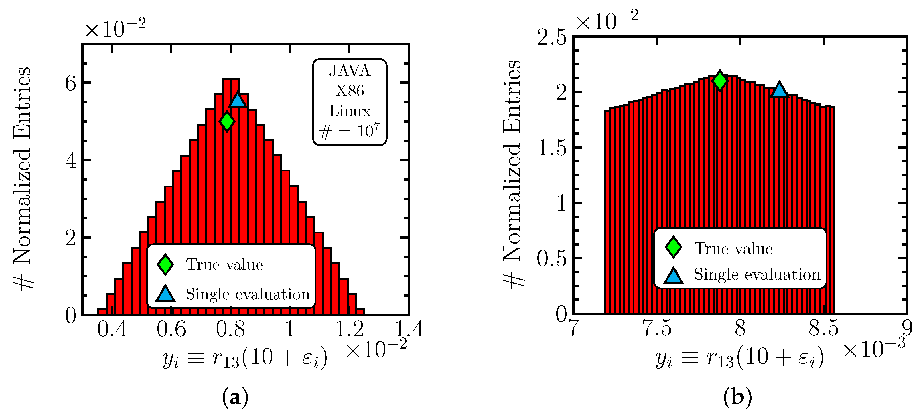
It may be interesting to examine the statistical distribution of $\left\{f^i\right\}$. Because all computing environments give similar results, we show only scenario C1 in Figure 1. One sees that the distribution is very symmetric but quite broad, meaning that the single evaluation (blue triangle) is close to its peak when compared to the distribution spread. Yet, in sub-figure (b), one observes that the peak of the distribution is significantly closer to the true value (green diamond) than the single evaluation result.

3.1.2. Second Example

We investigate a simple exponentiation implemented in an unstable manner:

$$\begin{array}{c}\hfill x^n=\left(2x\right)x^{n-2}+(x-2)x^{n-1}.\end{array}$$

Choosing $x=1/3$ and $n=15$, we compute $a_{15}=1/3^{15}$ using the recurrent relation

$$\begin{array}{c}\hfill a_n={\displaystyle \frac{2}{3}}{a}_{n-2}-{\displaystyle \frac{5}{3}}{a}_{n-1},a_1={\displaystyle \frac{1}{3}},a_2=a_1^2,\end{array}$$

(8)

where we perturb the value of $a_1$. We use $N={10}^6$ and $h={10}^{-7}$. The outcomes are shown in

Table 3. The precision of the evaluation of $a_{15}\left(1/3\right)$, Equation (8), by the averaging method compared to the direct evaluation for different computing environments (Table 1). Despite the large statistics for randomly generated $\left\{x_i\right\}$, the results have large fluctuations and cannot be reproduced exactly.

	$\mathit{f}\left(\mathit{x}\right)={\mathit{a}}_{15}\left(\mathit{x}\right)$, ${\mathit{x}}_0=1/3$, $\mathit{f}\left({\mathit{x}}_0\right)=0.00000006969171\dots$, $\mathit{h}={10}^{-7}$
	${▵}_{\mathbf{AV}}=\left|{\mathit{f}}_{\mathbf{AV}}\left({\mathit{x}}_{\mathbf{0}}\right)-\mathit{f}\left({\mathit{x}}_{\mathbf{0}}\right)\right|$	${▵}_{\mathbf{fl}}=\left|{\mathit{f}}_{\mathbf{fl}}\left({\mathit{x}}_{\mathbf{0}}\right)-\mathit{f}\left({\mathit{x}}_{\mathbf{0}}\right)\right|$	${▵}_{\mathbf{fl}}/{▵}_{\mathbf{AV}}$
C1	≈$2.4\times {10}^{-16}$	≈$7.3\times {10}^{-16}$	≈3
C2	≈$8.2\times {10}^{-17}$	≈$7.3\times {10}^{-16}$	≈8
C3	≈$9.9\times {10}^{-17}$	≈$7.3\times {10}^{-16}$	≈7
C4	≈$1.1\times {10}^{-16}$	≈$7.3\times {10}^{-16}$	≈7
C5	≈$8.0\times {10}^{-17}$	≈$7.6\times {10}^{-16}$	≈9
C6	≈$3.2\times {10}^{-16}$	≈$3.5\times {10}^{-14}$	≈110
C7	≈$2.4\times {10}^{-16}$	≈$7.3\times {10}^{-16}$	≈3
C8	≈$1.7\times {10}^{-16}$	≈$7.3\times {10}^{-16}$	≈4

, and, again, the validity of the averaging approach is demonstrated despite important fluctuations in the entries in the table (observed when attempting to reproduce them). The effect is, however, smaller than in the previous case.

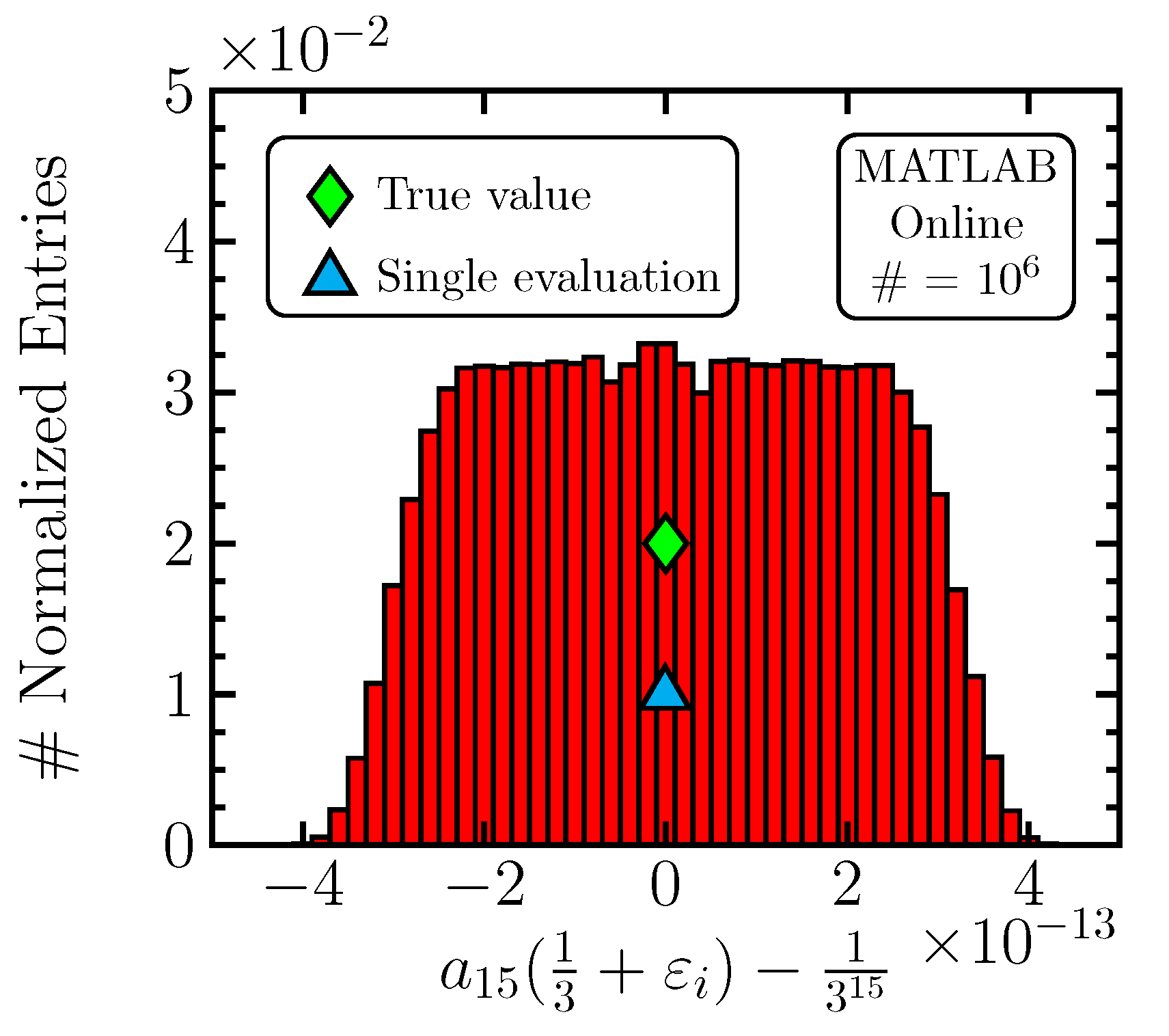
The error distribution for this computation in scenario C8 is shown in Figure 2.

The “simple function” examples fulfill the expectations that we have with respect to the method: we obtain a symmetric error distribution that provides, by averaging, a significant improvement in precision.

3.2. Matrix Inversion in Trigonometric Interpolation

In this section, we search for coefficients $c_{0,1,2,3}$ such that the trigonometric polynomial

$$f\left(x\right)=\sum _{n=0}^3{c}_{n}cos\left(nx\right)$$

(9)

interpolates ${\left\{\left(x_i,y_i\right)\right\}}_{i=0}^3$, with $x_i=1+i\times \Delta$, $\Delta ={10}^{-4}$ and $y_i=g\left(x_i\right)$, with

$$g\left(x\right)=-1-{\displaystyle \frac{1}{3}}cos\left(x\right)+{\displaystyle \frac{1}{7}}cos\left(2x\right)-{\displaystyle \frac{1}{11}}cos\left(3x\right).$$

Obviously, the correct values are $c_0=-1$, $c_1=-1/3$, $c_2=1/7$ and $c_3=-1/11$. The problem is written in a matrix form, $\overrightarrow{y}=M\overrightarrow{c}$, where

$$M_{ij}=cos\left(j{x}_i\right).$$

The task is to invert the matrix and find $\overrightarrow{c}$:

$$\overrightarrow{c}=M^{-1}\overrightarrow{y}.$$

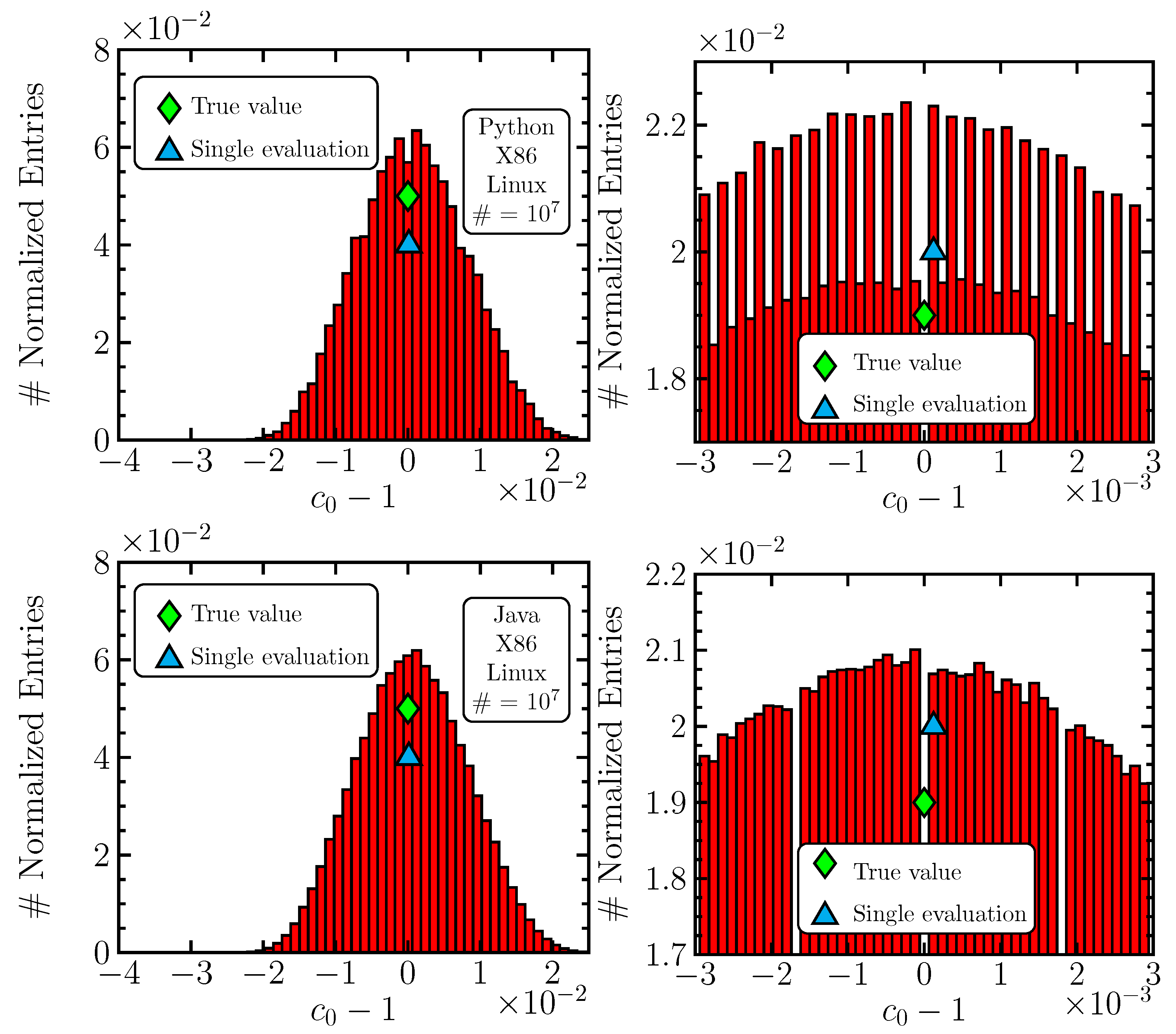
As a matter of fact, the problem is ill conditioned because $\Delta$ is small, and rows of M are very similar. Various strategies can be adopted when implementing perturbations: e.g., perturb the elements of M, those of y, or both. Every option can be studied, but here, we have chosen the first one, because the problem is often stated as “matrix inversion” alone, not necessarily related to some specific vector y. In each studied case, we independently perturb every element of M by a random amount, with all perturbations being from the same interval I. We observe that a typical perturbation (to obtain the best results) is significantly smaller than in the previous case (the $r_{13}$ function). The size of the statistical sample is $N={10}^5$. The code for matrix inversion differs considerably, depending on the programming language. For Java, we used the Jama “Matrix” library (https://math.nist.gov/javanumerics/jama/, accessed on 27 June 2024); for C(++), we borrowed a code published online (https://github.com/altafahmad623/Operation-Research/blob/master/inverse.c, accessed on 27 June 2024); for Python, the linalg library from the numpy package was called; and for JavaScript, we again referred to an implementation found online (https://web.archive.org/web/20210406035905/http://blog.acipo.com/matrix-inversion-in-javascript/, accessed on 27 June 2024). It turns out that the matrix inversion implementation is the most significant source of differences between various scenarios and, for the C(++) implementation, is unsatisfactory in the current setting due to producing nonsense numbers. For this reason, we make an exception and decrease, in this case, the condition number by setting $\Delta ={10}^{-3}$. Each result is represented by a set of four numbers, and the outcomes produced under various conditions are summarized in

Table 4. The precision of the evaluation of four trigonometric coefficients, Equation (9), by the averaging method, compared to the direct evaluation for different computing environments (Table 1). Despite the large statistics for randomly generated elements of M, the results have fluctuations and cannot be reproduced exactly.

	${\mathit{c}}_{\mathit{i}}\equiv {\left[\overrightarrow{\mathit{f}}\left(\mathit{M}\right)\right]}_{\mathit{i}}={\left[{\mathit{M}}^{-1}\overrightarrow{\mathit{y}}\right]}_{\mathit{i}}$
	${\mathit{f}}_{\mathbf{0}}=-\mathbf{1}$, ${\mathit{f}}_{\mathbf{1}}=-\mathbf{1}/\mathbf{3}$, ${\mathit{f}}_{\mathbf{2}}=\mathbf{1}/\mathbf{7}$, ${\mathit{f}}_{\mathbf{3}}=-\mathbf{1}/\mathbf{11}$
	${▵}_{\mathbf{AV}}^{\mathit{i}}=$	${▵}_{\mathbf{fl}}^{\mathit{i}}=$	${\mathit{R}}^{\mathit{i}}=$	$\mathit{h}$
	$\left|{\mathit{f}}_{\mathbf{AV}}{\left(\mathit{M}\right)}_{\mathit{i}}-\mathit{f}{\left(\mathit{M}\right)}_{\mathit{i}}\right|$	$\left|{\mathit{f}}_{\mathbf{fl}}{\left(\mathit{M}\right)}_{\mathit{i}}-\mathit{f}{\left(\mathit{M}\right)}_{\mathit{i}}\right|$	${▵}_{\mathbf{fl}}^{\mathit{i}}/{▵}_{\mathbf{AV}}^{\mathit{i}}$
C1	${▵}^0\approx 2.3\times {10}^{-5}$	${▵}^0\approx 1.8\times {10}^{-4}$	$R^0\approx 8$	${10}^{-14}$
	${▵}^1\approx 3.9\times {10}^{-5}$	${▵}^1\approx 2.0\times {10}^{-4}$	$R^1\approx 5$
	${▵}^2\approx 1.9\times {10}^{-5}$	${▵}^2\approx 1.6\times {10}^{-4}$	$R^2\approx 8$
	${▵}^3\approx 6.0\times {10}^{-6}$	${▵}^3\approx 2.8\times {10}^{-5}$	$R^3\approx 5$
C2	${▵}^0\approx 5.2\times {10}^{-3}$	${▵}^0\approx 1.0\times {10}^{-1}$	$R^0\approx 20$	${10}^{-12}$
$\Delta ={10}^{-3}$	${▵}^1\approx 6.4\times {10}^{-3}$	${▵}^1\approx 6.3\times {10}^{-1}$	$R^1\approx 100$
	${▵}^2\approx 3.8\times {10}^{-3}$	${▵}^2\approx 1.3$	$R^2\approx 340$
	${▵}^3\approx 3.4\times {10}^{-3}$	${▵}^3\approx 9.8\times {10}^{-2}$	$R^3\approx 30$
C3	${▵}^0\approx 1.4\times {10}^{-5}$	${▵}^0\approx 1.2\times {10}^{-4}$	$R^0\approx 8$	${10}^{-14}$
	${▵}^1\approx 2.4\times {10}^{-5}$	${▵}^1\approx 1.6\times {10}^{-4}$	$R^1\approx 7$
	${▵}^2\approx 1.3\times {10}^{-5}$	${▵}^2\approx 3.5\times {10}^{-5}$	$R^2\approx 3$
	${▵}^3\approx 4.1\times {10}^{-6}$	${▵}^3\approx 3.3\times {10}^{-5}$	$R^3\approx 8$
C4	${▵}^0\approx 3.3\times {10}^{-6}$	${▵}^0\approx 3.1\times {10}^{-5}$	$R^0\approx 9$	${10}^{-14}$
	${▵}^1\approx 5.5\times {10}^{-6}$	${▵}^1\approx 8.1\times {10}^{-5}$	$R^1\approx 14$
	${▵}^2\approx 2.9\times {10}^{-6}$	${▵}^2\approx 6.5\times {10}^{-5}$	$R^2\approx 22$
	${▵}^3\approx 8.5\times {10}^{-7}$	${▵}^3\approx 3.5\times {10}^{-5}$	$R^3\approx 41$
C5	${▵}^0\approx 2.6\times {10}^{-5}$	${▵}^0\approx 3.1\times {10}^{-5}$	$R^0\approx 1$	${10}^{-14}$
	${▵}^1\approx 4.3\times {10}^{-5}$	${▵}^1\approx 8.1\times {10}^{-5}$	$R^1\approx 2$
	${▵}^2\approx 2.2\times {10}^{-5}$	${▵}^2\approx 6.5\times {10}^{-5}$	$R^2\approx 3$
	${▵}^3\approx 6.8\times {10}^{-6}$	${▵}^3\approx 3.5\times {10}^{-5}$	$R^3\approx 5$
C6	${▵}^0\approx 2.9\times {10}^{-4}$	${▵}^0\approx 2.6\times {10}^{-1}$	$R^0\approx 890$	${10}^{-12}$
$\Delta ={10}^{-3}$	${▵}^1\approx 2.3\times {10}^{-3}$	${▵}^1\approx 1.9\times {10}^{-1}$	$R^1\approx 80$
	${▵}^2\approx 1.9\times {10}^{-3}$	${▵}^2\approx 3.5\times {10}^{-1}$	$R^2\approx 190$
	${▵}^3\approx 1.9\times {10}^{-4}$	${▵}^3\approx 6.5\times {10}^{-3}$	$R^3\approx 34$
C7	${▵}^0\approx 3.2\times {10}^{-5}$	${▵}^0\approx 3.1\times {10}^{-5}$	$R^0\approx 1$	${10}^{-14}$
	${▵}^1\approx 5.4\times {10}^{-5}$	${▵}^1\approx 8.1\times {10}^{-5}$	$R^1\approx 2$
	${▵}^2\approx 2.7\times {10}^{-5}$	${▵}^2\approx 6.5\times {10}^{-5}$	$R^2\approx 2$
	${▵}^3\approx 8.3\times {10}^{-6}$	${▵}^3\approx 3.5\times {10}^{-5}$	$R^3\approx 4$
C8	${▵}^0\approx 5.1\times {10}^{-6}$	${▵}^0\approx 6.1\times {10}^{-5}$	$R^0\approx 12$	${10}^{-15}$
	${▵}^1\approx 8.3\times {10}^{-6}$	${▵}^1\approx 2.0\times {10}^{-5}$	$R^1\approx 2$
	${▵}^2\approx 4.1\times {10}^{-6}$	${▵}^2\approx 1.6\times {10}^{-4}$	$R^2\approx 39$
	${▵}^3\approx 1.2\times {10}^{-6}$	${▵}^3\approx 1.8\times {10}^{-5}$	$R^3\approx 15$

. Illustrative error-distribution histograms for the $c_0$ coefficient are shown for the C1 and C3 scenarios in Figure 3. This time, the shape is Gaussian, and, surprisingly, the Python implementation manifests regular oscillatory structures, certainly a numerical effect, which is missing for Java. Still, both results are comparable since oscillations are also averaged.

The main conclusion that one can draw is that an increase in precision is observed with a significance of around one order of magnitude. Beyond doubt, this cannot be explained by statistical fluctuations, and the averaging method has an effect. The most important factor that determines the outcome is the implementation of the specific mathematical operation (matrix inversion, in our case), and, for an altered scenario with the C(++) code, the increase in precision is much more important (although the code’s performance is much lower because it cannot deal with $\Delta ={10}^{-4}$).

3.3. Higher-Order Derivatives

The numerical instability increases with the increasing derivative order, and at some point, any method of computation fails. It is interesting to see how various approaches behave in this respect. We obtain inspiration from [9] and differentiate

$$f\left(x\right)={\displaystyle \frac{e^x}{{\left(sinx\right)}^3+{\left(cosx\right)}^3}}$$

(10)

at $x=0$. All derivatives are integers, and we focus on the few first of them:

$${\left\{f^{\left(i\right)}\left(x\right){|}_{x=0}\right\}}_{i=1,2,3,4}=\left\{1,4,4,28\right\}.$$

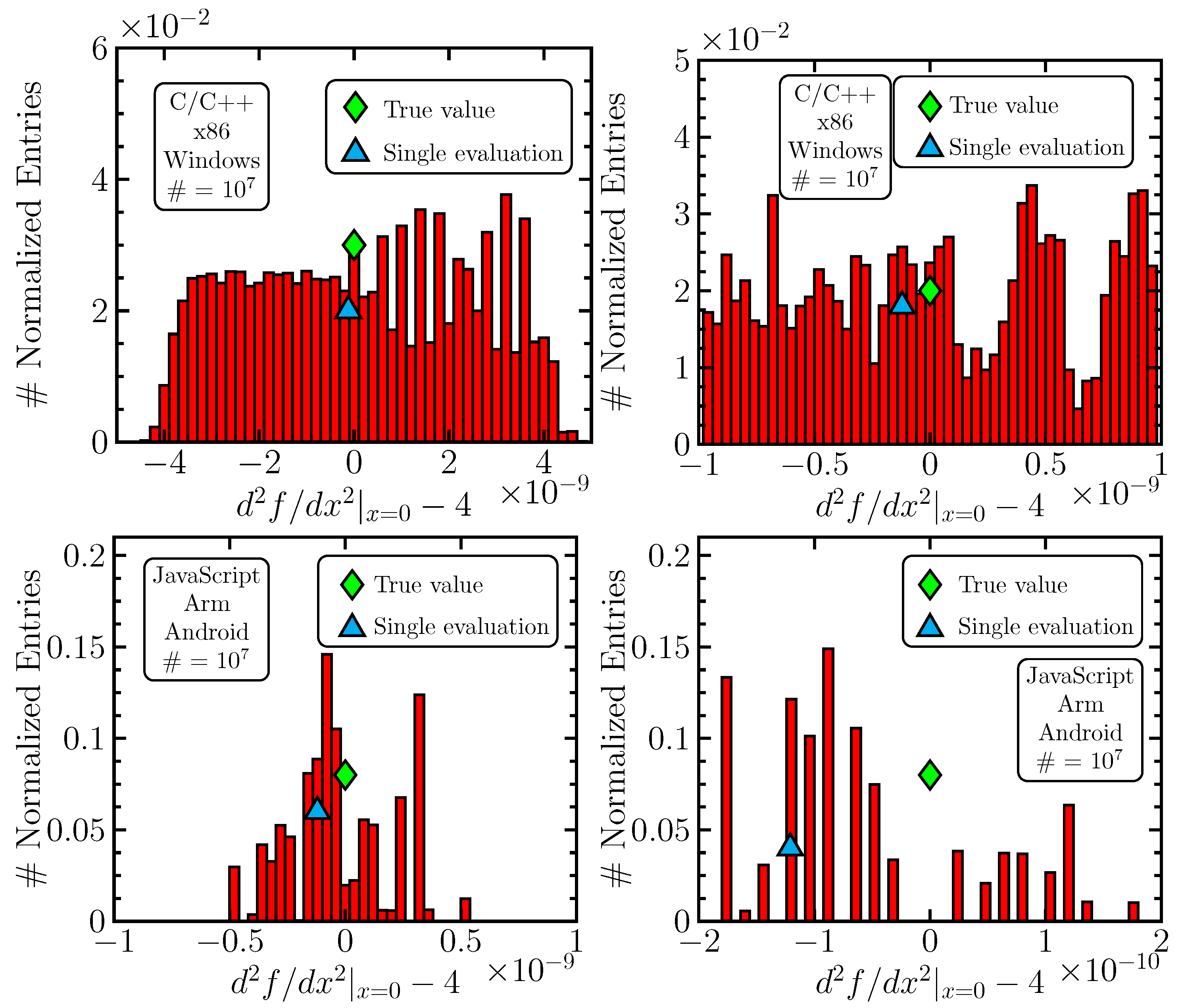
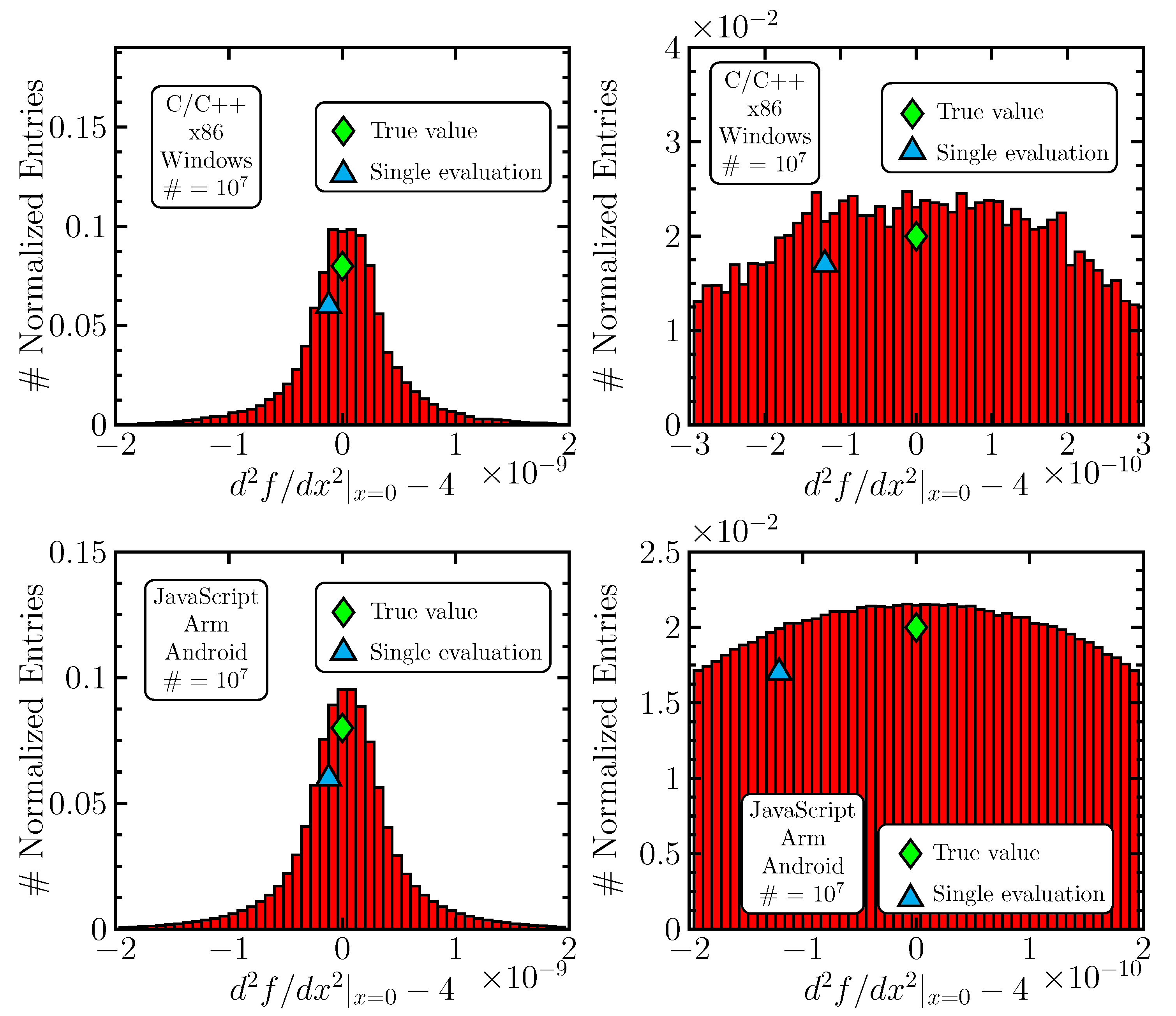
We use central difference formulas to obtain estimates; see

Table 5. Implemented central difference formulas with $y_n\equiv f(x_0+n\epsilon )$.

Deriv.	Formula
Order
1	$\left(y_{-2}/12-2y_{-1}/3+2y_1/3-y_2/12\right)/\epsilon$
2	$\left(-y_{-2}/12+4y_{-1}/3-5y_0/2+4y_1/3-y_2/12\right)/{\epsilon }^2$
3	$\left(y_{-3}/8-y_{-2}+13y_{-1}/8-13y_1/8+y_2-y_3/8\right)/{\epsilon }^3$
4	$\left(-y_{-3}/6+2y_2-13y_{-1}/2+28y_0/3-13y_1/2+2y_2-y_3/6\right)/{\epsilon }^4$

. The formulas depend on two parameters, $x_0$ and $\epsilon$, and we perturb both of them, one at a time, thus producing two result tables,

Table 6. Compared precision of averaging and single estimation for various derivative orders D. The argument x is perturbed randomly with the amplitude $h_x$. The finite-difference step is fixed to ${\epsilon }_0={10}^{-4}$ for $D=1$, ${\epsilon }_0={10}^{-3}$ for $D=2,3$ and ${\epsilon }_0={10}^{-2}$ for $D=4$. Despite the large statistics, the results fluctuate significantly and cannot be reproduced exactly.

	${\mathit{f}}^{\mathit{D}}\left(\mathit{x}\right)=\frac{{\mathit{d}}^{\mathit{D}}}{{\mathbf{dx}}^{\mathit{D}}}\left[{\mathit{e}}^{\mathit{x}}/\left({\left(sin\mathit{x}\right)}^3+{\left(cos\mathit{x}\right)}^3\right)\right]$
	${\mathit{f}}^{\mathbf{1}}\left(\mathbf{0}\right)=\mathbf{1}$, ${\mathit{f}}^{\mathbf{2}}\left(\mathbf{0}\right)=\mathbf{4}$, ${\mathit{f}}^{\mathbf{3}}\left(\mathbf{0}\right)=\mathbf{4}$, ${\mathit{f}}^{\mathbf{4}}\left(\mathbf{0}\right)=\mathbf{28}$
	$\mathit{x}$ Is Perturbed
	D	${▵}_{\mathbf{AV}}=$	${▵}_{\mathbf{fl}}=$	${▵}_{\mathbf{fl}}/{▵}_{\mathbf{AV}}$	${\mathit{h}}_{\mathit{x}}$
		$\left|{\mathit{f}}_{\mathbf{AV}}^{\mathit{D}}\left({\mathit{x}}_{\mathbf{0}}\right)-{\mathit{f}}^{\mathbf{D}}\left({\mathit{x}}_{\mathbf{0}}\right)\right|$	$\left|{\mathit{f}}_{\mathbf{fl}}^{\mathit{D}}\left({\mathit{x}}_{\mathbf{0}}\right)-{\mathit{f}}^{\mathit{D}}\left({\mathit{x}}_{\mathbf{0}}\right)\right|$
C1	1	≈$1.2\times {10}^{-13}$	≈$8.6\times {10}^{-13}$	≈7	${10}^{-14}$
	2	≈$4.8\times {10}^{-11}$	≈$1.2\times {10}^{-10}$	≈3	${10}^{-15}$
	3	≈$2.0\times {10}^{-8}$	≈$2.1\times {10}^{-9}$	≈1	${10}^{-8}$
	4	≈$1.2\times {10}^{-5}$	≈$1.4\times {10}^{-5}$	≈1	${10}^{-6}$
C2	1	≈$1.2\times {10}^{-13}$	≈$8.6\times {10}^{-13}$	≈7	${10}^{-14}$
	2	≈$4.8\times {10}^{-11}$	≈$1.2\times {10}^{-10}$	≈3	${10}^{-15}$
	3	≈$8.2\times {10}^{-10}$	≈$2.1\times {10}^{-9}$	≈3	${10}^{-8}$
	4	≈$1.4\times {10}^{-5}$	≈$1.4\times {10}^{-5}$	≈1	${10}^{-6}$
C3	1	≈$1.2\times {10}^{-13}$	≈$8.6\times {10}^{-13}$	≈7	${10}^{-14}$
	2	≈$4.8\times {10}^{-11}$	≈$1.2\times {10}^{-10}$	≈3	${10}^{-15}$
	3	≈$3.7\times {10}^{-10}$	≈$2.1\times {10}^{-9}$	≈6	${10}^{-8}$
	4	≈$1.3\times {10}^{-5}$	≈$1.4\times {10}^{-5}$	≈1	${10}^{-6}$
C4	1	≈$1.2\times {10}^{-13}$	≈$8.6\times {10}^{-13}$	≈7	${10}^{-14}$
	2	≈$4.8\times {10}^{-11}$	≈$1.2\times {10}^{-10}$	≈3	${10}^{-15}$
	3	≈$5.9\times {10}^{-10}$	≈$2.1\times {10}^{-9}$	≈4	${10}^{-8}$
	4	≈$1.4\times {10}^{-5}$	≈$1.4\times {10}^{-5}$	≈1	${10}^{-6}$
C5	1	≈$1.2\times {10}^{-13}$	≈$8.6\times {10}^{-13}$	≈7	${10}^{-14}$
	2	≈$4.7\times {10}^{-11}$	≈$1.2\times {10}^{-10}$	≈3	${10}^{-15}$
	3	≈$1.7\times {10}^{-9}$	≈$2.1\times {10}^{-9}$	≈1	${10}^{-8}$
	4	≈$1.4\times {10}^{-5}$	≈$1.4\times {10}^{-5}$	≈1	${10}^{-6}$
C6	1	≈$4.5\times {10}^{-13}$	≈$5.7\times {10}^{-13}$	≈1	${10}^{-11}$
	2	≈$2.6\times {10}^{-12}$	≈$1.3\times {10}^{-11}$	≈5	${10}^{-9}$
	3	≈$9.1\times {10}^{-10}$	≈$1.6\times {10}^{-7}$	≈180	${10}^{-8}$
	4	≈$1.4\times {10}^{-5}$	≈$1.4\times {10}^{-5}$	≈1	${10}^{-7}$
C7	1	≈$1.2\times {10}^{-13}$	≈$8.6\times {10}^{-13}$	≈7	${10}^{-14}$
	2	≈$4.7\times {10}^{-11}$	≈$1.2\times {10}^{-10}$	≈3	${10}^{-15}$
	3	≈$2.7\times {10}^{-9}$	≈$2.1\times {10}^{-9}$	≈1	${10}^{-8}$
	4	≈$1.4\times {10}^{-5}$	≈$1.4\times {10}^{-5}$	≈1	${10}^{-6}$
C8	1	≈$1.2\times {10}^{-13}$	≈$8.6\times {10}^{-13}$	≈7	${10}^{-14}$
	2	≈$4.7\times {10}^{-11}$	≈$1.2\times {10}^{-10}$	≈3	${10}^{-15}$
	3	≈$1.6\times {10}^{-9}$	≈$2.1\times {10}^{-9}$	≈1	${10}^{-8}$
	4	≈$1.4\times {10}^{-5}$	≈$1.4\times {10}^{-5}$	≈1	${10}^{-6}$

and

Table 7. The precision of the averaging and the single estimation compared for various derivative orders D. The argument $x=0$ is fixed. The finite-difference steps are perturbed around their central values ${\epsilon }_0$ using $h_{\epsilon }={\epsilon }_0/2$, and the displayed ${\epsilon }_0$ values are those used in the averaging method. Despite the large statistics, the results fluctuate significantly and cannot be reproduced exactly.

	${\mathit{f}}^{\mathit{D}}\left(\mathit{x}\right)=\frac{{\mathit{d}}^{\mathit{D}}}{{\mathbf{dx}}^{\mathit{D}}}\left[{\mathit{e}}^{\mathit{x}}/\left({\left(sin\mathit{x}\right)}^3+{\left(cos\mathit{x}\right)}^3\right)\right]$
	${\mathit{f}}^{\mathbf{1}}\left(\mathbf{0}\right)=\mathbf{1}$, ${\mathit{f}}^{\mathbf{2}}\left(\mathbf{0}\right)=\mathbf{4}$, ${\mathit{f}}^{\mathbf{3}}\left(\mathbf{0}\right)=\mathbf{4}$, ${\mathit{f}}^{\mathbf{4}}\left(\mathbf{0}\right)=\mathbf{28}$
	$\mathit{\epsilon }$ Is Perturbed
	D	${▵}_{\mathbf{AV}}=$	${▵}_{\mathbf{fl}}=$	${▵}_{\mathbf{fl}}/{▵}_{\mathbf{AV}}$	${\mathit{\epsilon }}_{\mathbf{0}}$
		$\left|{\mathit{f}}_{\mathbf{AV}}^{\mathit{D}}\left({\mathit{x}}_{\mathbf{0}}\right)-{\mathit{f}}^{\mathit{D}}\left({\mathit{x}}_{\mathbf{0}}\right)\right|$	$\left|{\mathit{f}}_{\mathbf{fl}}^{\mathit{D}}\left({\mathit{x}}_{\mathbf{0}}\right)-{\mathit{f}}^{\mathit{D}}\left({\mathit{x}}_{\mathbf{0}}\right)\right|$
C1	1	≈$3.8\times {10}^{-15}$	≈$8.6\times {10}^{-13}$	≈230	${10}^{-4}$
	2	≈$2.3\times {10}^{-12}$	≈$1.2\times {10}^{-10}$	≈52	${10}^{-3}$
	3	≈$8.1\times {10}^{-10}$	≈$2.1\times {10}^{-9}$	≈3	${10}^{-3}$
	4	≈$2.1\times {10}^{-5}$	≈$1.4\times {10}^{-5}$	≈$0.7$	${10}^{-2}$
C2	1	≈$3.5\times {10}^{-15}$	≈$8.6\times {10}^{-13}$	≈240	${10}^{-4}$
	2	≈$2.2\times {10}^{-12}$	≈$1.2\times {10}^{-10}$	≈55	${10}^{-3}$
	3	≈$2.6\times {10}^{-9}$	≈$2.1\times {10}^{-9}$	≈$0.8$	${10}^{-3}$
	4	≈$2.1\times {10}^{-5}$	≈$1.4\times {10}^{-5}$	≈$0.7$	${10}^{-2}$
C3	1	≈$1.8\times {10}^{-15}$	≈$8.6\times {10}^{-13}$	≈484	${10}^{-4}$
	2	≈$4.1\times {10}^{-13}$	≈$1.2\times {10}^{-10}$	≈300	${10}^{-3}$
	3	≈$2.6\times {10}^{-9}$	≈$2.1\times {10}^{-9}$	≈$0.8$	${10}^{-3}$
	4	≈$2.1\times {10}^{-5}$	≈$1.4\times {10}^{-5}$	≈$0.7$	${10}^{-2}$
C4	1	≈$2.2\times {10}^{-15}$	≈$8.6\times {10}^{-13}$	≈390	${10}^{-4}$
	2	≈$9.4\times {10}^{-13}$	≈$1.2\times {10}^{-10}$	≈130	${10}^{-3}$
	3	≈$5.4\times {10}^{-10}$	≈$2.1\times {10}^{-9}$	≈4	${10}^{-3}$
	4	≈$2.1\times {10}^{-5}$	≈$1.4\times {10}^{-5}$	≈$0.7$	${10}^{-2}$
C5	1	≈$2.0\times {10}^{-15}$	≈$8.6\times {10}^{-13}$	≈431	${10}^{-4}$
	2	≈$1.9\times {10}^{-12}$	≈$1.2\times {10}^{-10}$	≈64	${10}^{-3}$
	3	≈$1.9\times {10}^{-9}$	≈$2.1\times {10}^{-9}$	≈1	${10}^{-3}$
	4	≈$2.1\times {10}^{-5}$	≈$1.4\times {10}^{-5}$	≈$0.7$	${10}^{-2}$
C6	1	≈$3.5\times {10}^{-15}$	≈$5.7\times {10}^{-13}$	≈160	${10}^{-4}$
	2	≈$3.4\times {10}^{-12}$	≈$1.3\times {10}^{-11}$	≈4	${10}^{-3}$
	3	≈$1.6\times {10}^{-9}$	≈$1.6\times {10}^{-7}$	≈100	${10}^{-3}$
	4	≈$1.7\times {10}^{-5}$	≈$1.4\times {10}^{-5}$	≈$0.8$	${10}^{-2}$
C7	1	≈$3.1\times {10}^{-15}$	≈$8.6\times {10}^{-13}$	≈280	${10}^{-4}$
	2	≈$2.2\times {10}^{-12}$	≈$1.2\times {10}^{-10}$	≈55	${10}^{-3}$
	3	≈$2.1\times {10}^{-9}$	≈$2.1\times {10}^{-9}$	≈1	${10}^{-3}$
	4	≈$2.1\times {10}^{-5}$	≈$1.4\times {10}^{-5}$	≈$0.7$	${10}^{-2}$
C8	1	≈$2.7\times {10}^{-15}$	≈$8.6\times {10}^{-13}$	≈320	${10}^{-4}$
	2	≈$3.6\times {10}^{-12}$	≈$1.2\times {10}^{-10}$	≈33	${10}^{-3}$
	3	≈$9.9\times {10}^{-10}$	≈$2.1\times {10}^{-9}$	≈2	${10}^{-3}$
	4	≈$2.1\times {10}^{-5}$	≈$1.4\times {10}^{-5}$	≈$0.7$	${10}^{-2}$

. Perturbing $x_0=0$ is straightforward, and $\epsilon$ is perturbed around the optimal value ${\epsilon }_0={10}^{-k}$, which we find by applying the averaging method for an integer k. Similarly, we compute derivatives (single estimations) at zero, testing different integers k, and, by comparing them to the true values, we choose the best. The values in the averaging approach are perturbed randomly in the interval ${\epsilon }_i\in ({\epsilon }_0/2,3\times {\epsilon }_0/2)$. We set the statistics to $N={10}^5$. As illustrative examples, we provide histograms for error distributions of the second derivative for the C5 and C6 scenarios in Figure 4 and Figure 5.

One sees that the averaging method provides an improvement in precision for the first two derivatives, which is generally lost for the third and fourth derivatives. Also, the perturbation in $\epsilon$ gives more important improvements. It is necessary to understand why the method fails above the second derivative, and we provide, in what follows, a dedicated section to this issue.

The better performance of the $\epsilon$-based approach may be qualitatively understood, since the smallness of the $\epsilon$ parameter causes catastrophic cancellation; i.e., if $\epsilon$ is big, then no instability will be present, even for small x-perturbations. Thus, by varying ${\epsilon }_0$ in the finite difference $\left[f\left(x_0+{\epsilon }_0\right)-f\left(x_0\right)\right]/{\epsilon }_0$ (as an example), a large number of various values are created, forming an approximate Gaussian, and can be averaged (Figure 5). Performing a shift in x, i.e., varying ${\delta }_x$ in $\left[f\left(x_0+{\delta }_x+{\epsilon }_0\right)-f\left(x_0+{\delta }_x\right)\right]/{\epsilon }_0$ with ${\epsilon }_0$ fixed, computes function values at two points, which always have the same distance, ${\epsilon }_0$. The function value differences then tend to be strongly correlated, and a linear function gives a constant. At the scale ${10}^{-15}\lesssim h_x\lesssim {10}^{-6}$ (see Table 6), the function (10) is well described by its linear approximation; the small deviation from linearity (and possibly rounding effects) leads to a limited number of floating-point values that the finite difference can take and that are, in addition, unevenly distributed (Figure 4). Nevertheless, one also observes some differences between the upper and lower pictures in Figure 5, which indicates that the computing environment also plays a role, because the program codes are more or less equivalent in all scenarios. Another interesting observation is the third derivative in the C6 scenario in both Table 6 and Table 7; the precision is significantly increased (unlike in all other scenarios) and is even greater than for the second derivative in the same case. We do not have an understanding of this effect but see it as a further confirmation of the fact that the computing environment may induce important and unpredictable changes in results.

4. Fourth Derivative

For space and brevity reasons, we do not perform an exhaustive search including all scenarios and analyze the problem only in the C1 case (Java, Linux, x86) by perturbing $\epsilon$. We believe that the generalization of our findings is valid, yet, for further confirmation, this issue may be subject to additional studies in the future.

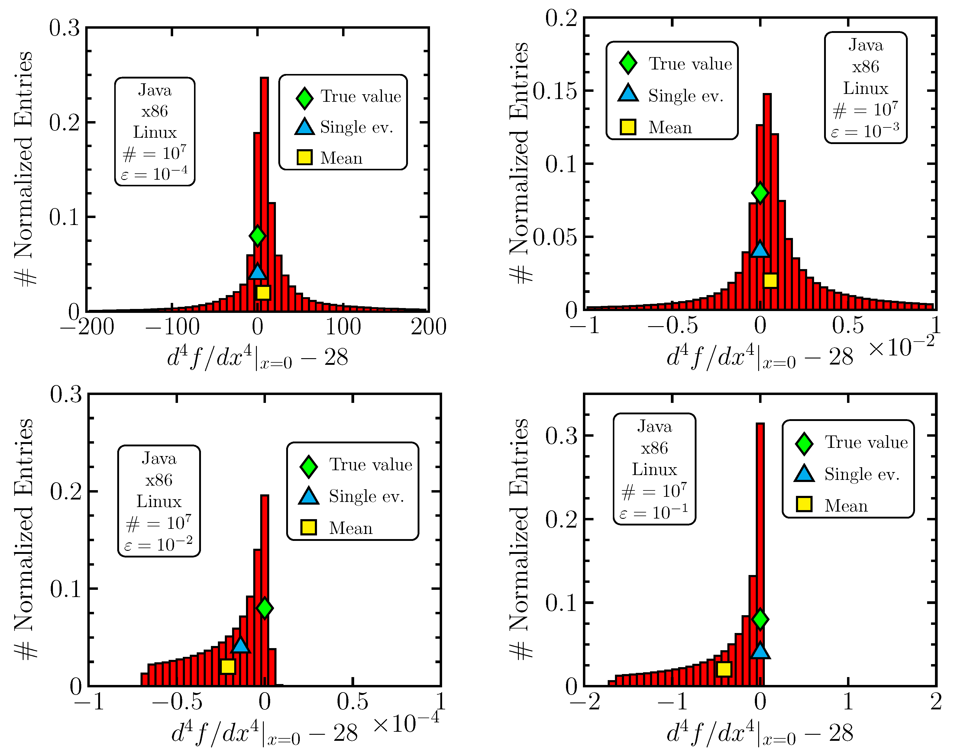
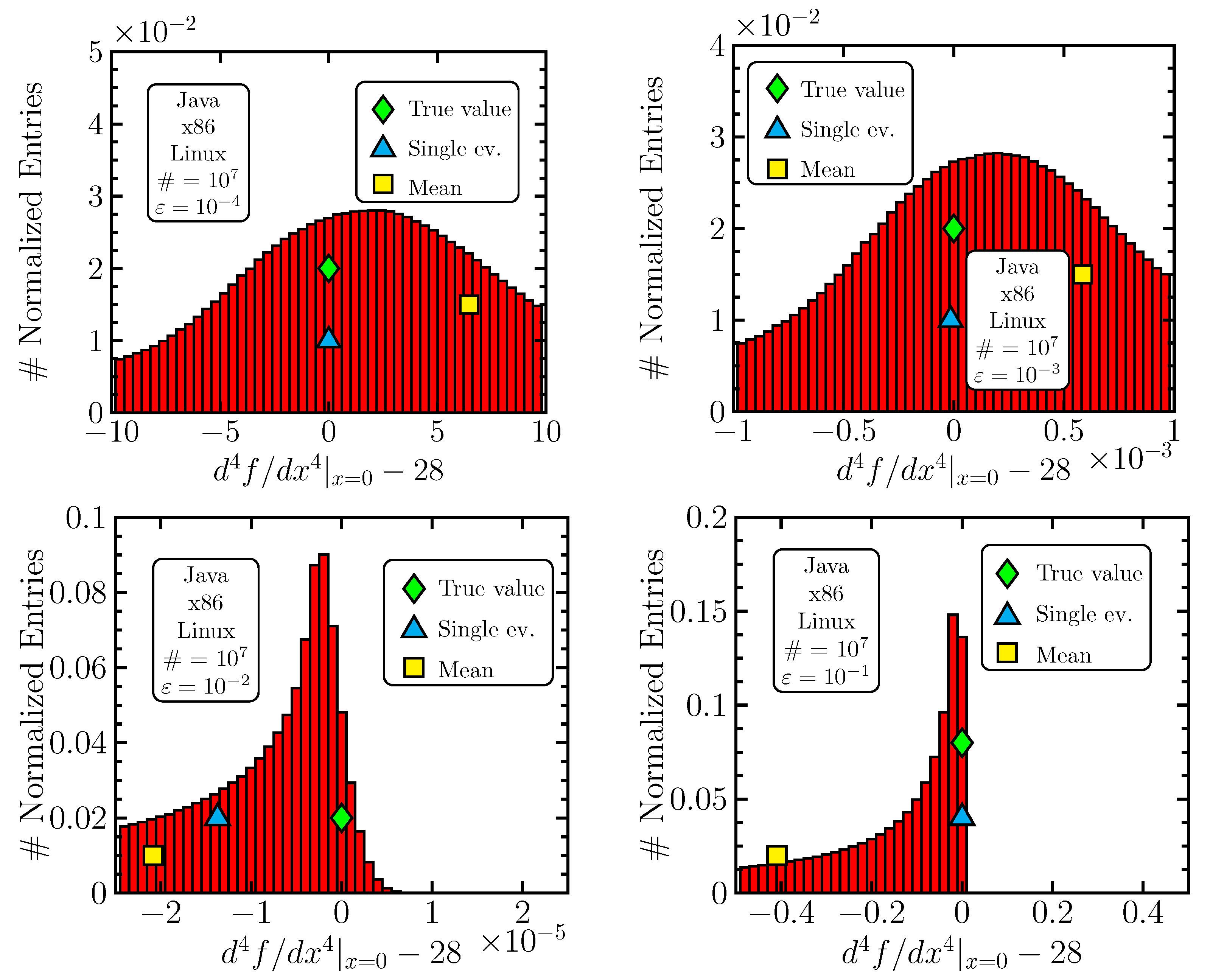
We learn the most by looking at the error histograms. We produced a few of them using ${\epsilon }_0^{\mathrm{new}}={\epsilon }_0/100$, ${\epsilon }_0/10$, ${\epsilon }_0$ and $10\times {\epsilon }_0$ with ${\epsilon }_0={10}^{-2}$ (see Table 7); a larger variation, $100\times {\epsilon }_0$, already hits the closest singularity of (10) at $x=-\pi /4$ and leads to strongly disturbed results. The histograms are shown in Figure 6 and their zoomed-in versions in Figure 7. The impact of round-off errors is most easily assessed by (practically) removing them using arbitrary-precision software. In our case, we benefited from the Apfloat library (http://www.apfloat.org/, accessed on 27 June 2024) using 300 valid decimal digits and $N=1000$ (and higher). Also, we did not use a random generation of ${\epsilon }_i\in ({\epsilon }_0/2,3\times {\epsilon }_0/2)$ but regularly divided the interval and performed calculation scanning with the step ${\epsilon }_0/N$. This was carried out with the aim of removing the possible bias from a non-ideal random number generator. This may introduce another bias, which would be, however, uncorrelated. The round-off-error-free histograms are presented in Figure 8.

The mere description of what one sees in Figure 6 and Figure 7 is that the distributions are shifted (the mean of the histogram is represented by the yellow square) and sometimes highly asymmetric. One also observes that the spread of the distribution changes dramatically when changing the discretization parameter ${\epsilon }_0$. When compared to Figure 8, it becomes clear what is going on. For small ${\epsilon }_0={10}^{-3},{10}^{-4}$, round-off errors appear and make the distribution more symmetric (as we argued), with, however, a (very) large spread. All distributions have some systematic shift, as seen from plots in Figure 8, which, however, decreases (as expected) with decreasing ${\epsilon }_0$. Despite the true value lying in the most probable bin, it is positioned at the edge of the distribution, which makes averaging ineffective. Nevertheless, it is still competitive in precision for ${\epsilon }_0={10}^{-2}$: the fact that the averaging method “loses” can be interpreted as random bad luck; the single-evaluation value (blue triangle, bottom-left graphics in Figure 6) could have been (if interpreted as random, with the histogram representing the probability distribution function) situated left to the mean. Nevertheless, it is clear that averaging is unable to provide any substantial improvement. For both values ${\epsilon }_0={10}^{-2},{10}^{-1}$, the round-off effects lose significance, yet a notable rise in bias and spread appears.

As a general assertion, one may say that for very unstable computations, changes in the tested sizes of perturbations (we used a discrete set of the form ${10}^{-n}$) may lead to a steep rise in the systematic bias (which cannot be averaged) and distribution widths. Here, one should distinguish between two cases:

• The perturbation can be zero, i.e., the true value can be reached, such as in Section 3.1.
• The perturbation cannot reach zero, such as the discretization parameter in derivative estimates.

In the second situation, the choice of some perturbation (e.g., ${\epsilon }_0={10}^{-n}$, $h_{\epsilon }={\epsilon }_0/2$) may be too small, so the round-off effects dominate. The next, larger choice (e.g., ${\epsilon }_0={10}^{-n+1}$, $h_{\epsilon }={\epsilon }_0/2$) may already be too big, so a significant bias is induced, implying that the region (interval) where the values of the parameter give reasonable results is very small. The first situation is similar: the interval that provides reasonable estimates may be very small around the true value, and going beyond it means a steep rise in the bias and distribution widths. In both scenarios, one can try to make the averaging approach work in this small interval.

In conclusion, we presume that the failure of the averaging approach is generally related to strong variations in the bias and width of the error distribution when perturbing the argument. This causes the interval of possible values of perturbations ${\delta }_i$ to be very small, conflicting with the fact that the machine numbers have non-zero spacing. The distributions to be averaged are then unevenly populated and strongly impaired by numerical effects, sometimes containing only a limited number of discrete values. If a perturbation from outside this interval is used, then other effects that are not round-off-error-related may appear and cause a systematic shift. Further interesting questions related to this topic are discussed in Appendix B.

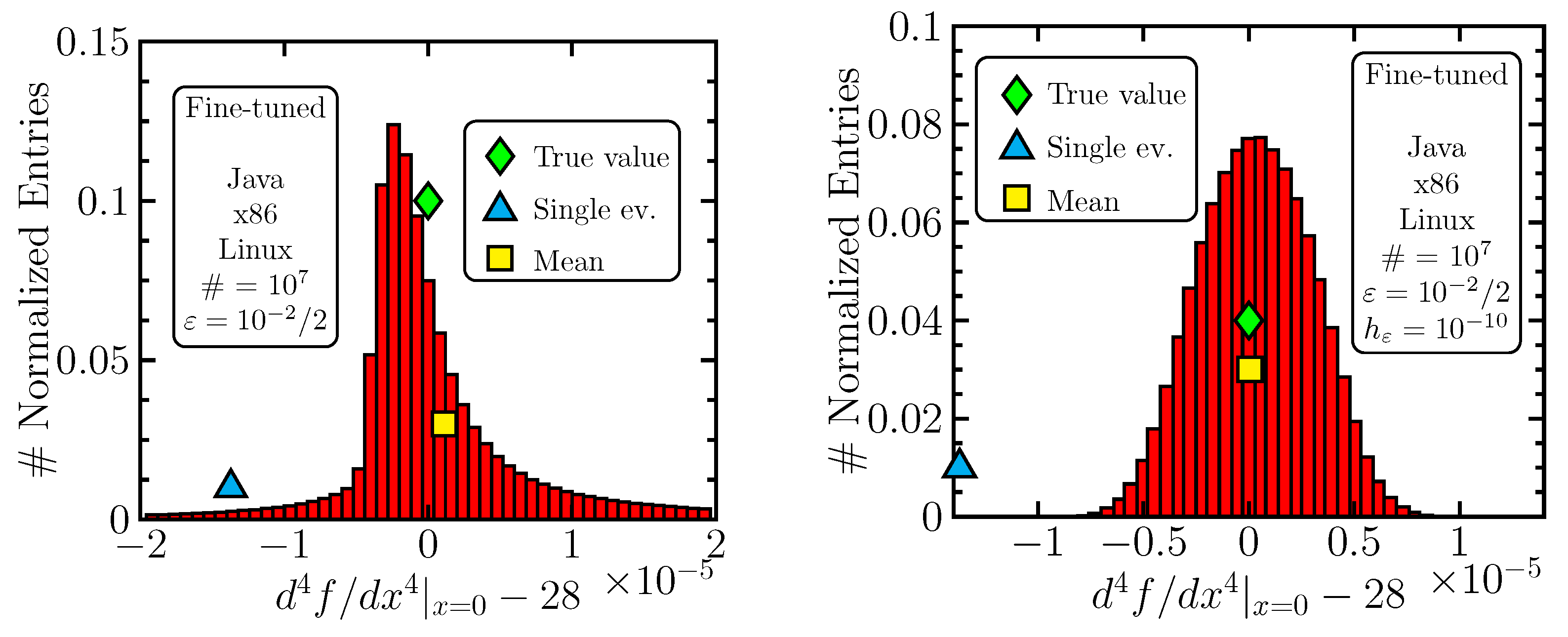
At last, let us perform a simple test: if we change the mean size of the discretization parameter ${\epsilon }_0$, we also change, by our convention, the amplitude of its perturbations $h_{\epsilon }={\epsilon }_0/2$, i.e., ${\epsilon }_i\in ({\epsilon }_0-h_{\epsilon },{\epsilon }_0+h_{\epsilon })=({\epsilon }_0/2,3\times {\epsilon }_0/2)$. The average size of the perturbation and, consequently, the length of the interval from which ${\epsilon }_i$ values are taken are thus adjusted automatically once the choice of ${\epsilon }_0$ is made. The latter takes the form ${\epsilon }_0={10}^{-n}$, which was chosen for a reason: in a black-box scenario, without the knowledge of the true values, one might only guess which ${\epsilon }_0$ is desirable and cannot fine-tune. Keeping this in mind, we do not want our results to appear fine-tuned, so the step between the consecutive sizes that we tested is rather big. Let us now allow for some fine-tuning and see what happens for ${\epsilon }_0={10}^{-2}/2$. The results are $(N={10}^7)$

$$\begin{array}{cc}\hfill {▵}_{\mathrm{AV}}& \approx 1.12\times {10}^{-6},{▵}_{\mathrm{fl}}\approx 13.7\times {10}^{-6},{▵}_{\mathrm{fl}}/{▵}_{\mathrm{AV}}\approx 12.19.\hfill \end{array}$$

The effect is there: averaging “wins”, and only the appropriate averaging interval went unnoticed by our ${\epsilon }_0={10}^{-n}$ scanning radar. The error histogram is shown in Figure 9—left.

The effect can be strongly amplified if we break our convention: by choosing a smaller value for $h_{\epsilon }={10}^{-10}$, we significantly shorten the interval of the used perturbations ${\epsilon }_i\in ({10}^{-2}/2-{10}^{-10},{10}^{-2}/2+{10}^{-10})$. One notices that the length of this interval is still much greater than computer precision. We obtain

$$\begin{array}{cc}\hfill {▵}_{\mathrm{AV}}& \approx 4.7\times {10}^{-8},{▵}_{\mathrm{fl}}\approx 1.4\times {10}^{-5},{▵}_{\mathrm{fl}}/{▵}_{\mathrm{AV}}\approx 290.\hfill \end{array}$$

See Figure 9—right.

5. Summary, Discussion, Conclusions and Outlook

As shown throughout this work, averaging, meant as a tool for suppressing round-off errors in unstable calculations, is effective. For this, we have provided theoretical support and several numerical experiments. If we have the means to fine-tune the size of perturbations and possibly other parameters (the step in differentiation), then in almost every numerical problem, one can choose such values as to outperform the single evaluation in precision. It may happen that the length of the interval around the true (or optimal) value, where the bias and width of the error distributions remain small, is very short and can be compared to the spacing of the floating-point numbers. Then, the averaging approach may suffer from severe numerical effects and may not provide an improvement (but remains competitive).

Averaging can be used in a scenario where any prior information (about the function or numerical effects) is poor, and the question about the optimal size of perturbations is difficult to answer. It seems safe to use perturbations that are small but greater (by an order of magnitude) than the smallest possible one (for a given floating-point arithmetic). With such a choice, an improvement is expected, yet it may be far from the optimal choice. One may also attempt to derive theoretical estimates if at least some constraints are available (bounds on the function and its derivatives); this is our outlook. Still, the safest approach for a given computation is probably to study special cases of this computation or problems that are computationally very similar and have known answers so that the amplitude of perturbations can be tuned.

Nevertheless, our goal is mainly to give a theoretical message, which, despite its simple underlying idea, is not found in the literature. Even so, this does not exclude practical applications of the method in some rare situations. This depends on the circumstances rather than on the method itself. It may happen that a numerical model that one uses and relies on is available only as an executable, without the source code and without the knowledge of its theoretical background. Then, averaging based on perturbing its input parameters may be the only way to increase the precision, if necessary. This could possibly also apply to situations where knowledge is available, but re-programming (let us say in an arbitrary-precision language) is costly. Some quantities (such as the first derivative) are improved significantly by the averaging method (Table 7), which may improve the practical application potential of averaging for such cases.

In this text, we have put the emphasis on the computing environment, and it indeed has an impact. These effects, complemented by other numerical effects, lead to various observations:

• Many numbers in the result tables have substantial fluctuations, as observed when reproducing them. This is in spite of the large statistic that is used.
• Distribution shapes vary: sometimes triangular (Figure 1) and sometimes Gaussian (Figure 5) or other.
• Changing the computational environment may make numerical disturbances (dis)appear. An example is the regular peaky structure seen in the upper-right picture in Figure 3.
• The third derivative is, for some reason, surprisingly precise for the C6 case (C++, Windows).

We do not have an understanding of these effects. Acquiring it would entail tedious work studying low-level computer arithmetic. But, this is not necessary for our purposes: these effects exist, and the averaging approach is cross-platform valid thanks to its robust, statistical character.

Being persuaded that averaging is an existing numerical phenomenon that one can possibly profit from, there are many different directions in which one could investigate it further. One could, for example, search for rules to properly set the averaging parameters for higher-order derivatives, since somewhat disappointing numbers for $D=3,4$ in Table 7 can certainly be improved, as demonstrated in Section 4.

References

1. Liptaj, A. Statistical approach for highest precision numerical differentiation. Math. Comput. Simul. 2023, 203, 92–111. [Google Scholar] [CrossRef]
2. Hull, T.E.; Swenson, J.R. Tests of probabilistic models for propagation of roundoff errors. Commun. ACM 1966, 9, 108–113. [Google Scholar] [CrossRef]
3. Linnainmaa, S. Towards accurate statistical estimation of rounding errors in floating-point computations. BIT 1975, 15, 165–173. [Google Scholar] [CrossRef]
4. Brunet, M.C.; Chatelin, F. A probabilistic round-off error propagation model, application to the eigenvalue problem. In Reliable Numerical Commputation; Oxford Academic: Oxford, UK, 1990; pp. 139–160. [Google Scholar] [CrossRef]
5. Higham, N.J.; Mary, T. A new approach to probabilistic rounding error analysis. SIAM J. Sci. Comput. 2019, 41, A2815–A2835. [Google Scholar] [CrossRef]
6. IEEE Std 754-2019 (Revision of IEEE 754-2008); IEEE Standard for Floating-Point Arithmetic. IEEE: New York, NY, USA, 2019.
7. Kahan, W. Pracniques: Further remarks on reducing truncation errors. Commun. ACM 1965, 8, 40. [Google Scholar] [CrossRef]
8. Miel, G. Calculator calculus and roundoff errors. Am. Math. Mon. 1980, 87, 243–252. [Google Scholar] [CrossRef]
9. Fornberg, B. Numerical differentiation of analytic functions. ACM Trans. Math. Softw. 1981, 7, 512–526. [Google Scholar] [CrossRef]
Figure 1. Area-normalized statistical distribution of r 13 ( 10 + δ i ) for random δ i uniformly distributed over 10 4 , 10 4 , sub-figure (a). The peak area is enlarged in sub-figure (b).
Axioms 13 00615 g001
Figure 2. Area-normalized statistical distribution of a 15 ( 1 / 3 + δ i ) 1 / 3 15 for random δ i uniformly distributed over 10 7 , 10 7 for the C8 scenario.
Axioms 13 00615 g002
Figure 3. Area-normalized distributions of errors of the c 0 coefficient (9) around the true value with the averaging method, as observed for Python (first row, C3 setting) and Java (second row, C1 setting). In both cases, some numerical issues are observed. In the second column, the peak region is magnified.
Axioms 13 00615 g003
Figure 4. Area-normalized error distributions of the second-derivative estimates of (10) in the C5 (lower row) and C6 (upper row) scenarios perturbing x. In the pictures on the right, the peak area is enlarged.
Axioms 13 00615 g004
Figure 5. Area-normalized error distributions of the second-derivative estimates of (10) in the C5 (lower row) and C6 (upper row) scenarios perturbing the discretization parameter ε . In the pictures on the right, the peak area is enlarged.
Axioms 13 00615 g005
Figure 6. Area-normalized distributions of errors on the fourth derivative of (10) at zero in the C1 setting for various sizes of the mean value of the discretization parameter ε 0 (around which perturbations are randomly produced). One can note large changes in scale on the x-axis.
Axioms 13 00615 g006
Figure 7. Distributions identical to those in Figure 6 but enlarged in the central area.
Axioms 13 00615 g007
Figure 8. Modifications of distributions from Figure 6 with round-off errors (practically) removed.
Axioms 13 00615 g008
Figure 9. Area-normalized distributions of the fourth-derivative error for function (10) produced with ε 0 = 10 2 / 2 and with h ε = 10 2 / 4 (left) and h ε = 10 10 (right).
Axioms 13 00615 g009