Article

Probabilistic Perturbation Bounds for Invariant, Deflating and Singular Subspaces

Department of Engineering Sciences, Bulgarian Academy of Sciences, 1040 Sofia, Bulgaria
Axioms 2024, 13(9), 597; https://doi.org/10.3390/axioms13090597
Submission received: 22 July 2024 / Revised: 17 August 2024 / Accepted: 21 August 2024 / Published: 2 September 2024
(This article belongs to the Special Issue New Trends in Discrete Probability and Statistics)

Abstract

:
In this paper, we derive new probabilistic bounds on the sensitivity of invariant subspaces, deflation subspaces and singular subspaces of matrices. The analysis exploits a unified method for deriving asymptotic perturbation bounds of the subspaces under interest and utilizes probabilistic approximations of the entries of random perturbation matrices implementing the Markoff inequality. As a result of the analysis, we determine with a prescribed probability asymptotic perturbation bounds on the angles between the corresponding perturbed and unperturbed subspaces. It is shown that the probabilistic asymptotic bounds proposed are significantly less conservative than the corresponding deterministic perturbation bounds. The results obtained are illustrated by examples comparing the known deterministic perturbation bounds with the new probabilistic bounds.

1. Introduction

In this paper, we are concerned with the derivation of realistic perturbation bounds on the sensitivity of various important subspaces arising in matrix analysis. Such bounds are especially needed in the perturbation analysis of high dimension subspaces when the known bounds may produce very pessimistic results. We show that much tighter bounds on the subspace sensitivity can be obtained by using a probabilistic approach based on the Markoff inequality.
The sensitivity of invariant, deflation and singular subspaces of matrices is considered in detail in the fundamental book of Stewart and Sun [1], as well as in the surveys of Bhatia [2] and Li [3]. In particular, perturbation analysis of the eigenvectors and invariant subspaces of matrices affected by deterministic and random perturbations is presented in several papers and books, see for instance [4,5,6,7,8,9,10,11,12]. Survey [13] is entirely devoted to the asymptotic (first-order) perturbation analysis of eigenvalues and eigenvectors. The algorithmic and software problems in computing invariant subspaces are discussed in [14]. The sensitivity of deflating subspaces arising in the generalized Schur decomposition is considered in [15,16,17,18], and numerical algorithms for analyzing this sensitivity are presented in [19]. Bounds on the sensitivity of singular values and singular spaces of matrices that are subject to random perturbations are derived in [20,21,22,23,24,25,26], to name a few. The stochastic matrix theory that can be used in case of stochastic perturbations is developed in the papers of Stewart [27], and Edelman and Rao [28].
In [29], the author proposed new componentwise perturbation bounds of unitary and orthogonal matrix decomposition based on probabilistic approximations of the entries of random perturbation matrices implementing the Markoff inequality. It was shown that using such bounds it is possible to decrease significantly the asymptotic perturbation bounds of the corresponding similarity or equivalence transformation matrices. Based on the probabilistic asymptotic estimates of the entries of random perturbation matrices, presented in [29], in this paper we derive new new probabilistic bounds on the sensitivity of invariant subspaces, deflation subspaces and singular subspaces of matrices. The analysis and the examples given demonstrate that, in contrast to the known deterministic bounds, the probabilistic bounds are much tighter with a sufficiently high probability. The analysis performed exploits a unified method for deriving asymptotic perturbation bounds of the subspaces under interest, developed in [30,31,32,33,34], and utilizes probabilistic approximations of the entries of random perturbation matrices implementing the Markoff inequality. As a result of the analysis, we determine, with a prescribed probability, asymptotic perturbation bounds on the angles between the perturbed and unperturbed subspaces. It is proved that the new probabilistic asymptotic bounds are significantly less conservative than the corresponding deterministic perturbation bounds. The results obtained are illustrated by examples comparing the deterministic perturbation bounds derived by Stewart [16,35] and Sun [11,18] with the probabilistic bounds derived in this paper.
The paper is structured as follows. In Section 2, we briefly present the main results concerning the derivation of lower magnitude bounds on the entries of a random matrix using only its Frobenius norm. In the next three sections, Section 3, Section 4 and Section 5, we show the application of this approach to derive probabilistic perturbation bounds for the invariant, deflating and singular subspaces of matrices, respectively. We illustrate the theoretical results by examples demonstrating that the probability bounds of such subspaces are much tighter than the corresponding deterministic asymptotic bounds. We note that the known deterministic bounds for the invariant, deflating and singular subspaces are presented briefly as theorems without proof, only with the purpose to compare them with the new bounds.
All computations in the paper are performed with MATLAB® Version 9.9 (R2020b) [36] using IEEE double-precision arithmetic. M-files implementing the perturbation bounds described in the paper can be obtained from the author.

2. Probabilistic Bounds for Random Matrices

Consider an m × n random matrix, δ A , with uncorrelated elements. In the componentwise perturbation analysis of matrix decompositions, we have to use a matrix bound Δ A = [ Δ a i j ] , Δ a i j > 0 , so that | δ A | Δ A , i.e.,
| δ a i j | Δ a i j , i = 1 , 2 , , m , j = 1 , 2 , , n ,
where Δ a i j = δ A and . is some matrix norm. However, if for instance we use the Frobenius norm of δ A , we have that Δ a i j = δ A F and
Δ A F = m n δ A F ,
which produces very pessimistic results for a large m and n. To reduce Δ A F , in [29] it is proposed to decrease the entries of Δ A , taking a bound with entries Δ a i j = δ A F / Ξ , where Ξ > 1 . Of course, in the general case, such a bound will not satisfy (1) for all i and j. However, we can allow to exist some entries, δ a i j , of the perturbation δ A that exceed in magnitude, with some prescribed probability, the corresponding bound, Δ a i j . This probability can be determined by the Markoff inequality ([37], Section 5-4)
P { ξ a } E { ξ } a ,
where P { ξ a } is the probability that the random variable ξ is greater or equal to a given number, a, and E { ξ } is the average (or mean value) of ξ . Note that this inequality is valid for arbitrary distribution of ξ , which makes it conservative for a specific probability distribution. Applying the Markoff inequality, with ξ equal to the entry | δ a i j | and a equal to the corresponding bound Δ a i j , we obtain the following result [29].
Theorem 1. 
For an m × n random perturbation, δ A , and a desired probability 0 < P r e f < 1 , the estimate Δ A = [ Δ a i j ] , where
Δ a i j = δ A F Ξ ,
and
Ξ = ( 1 P r e f ) m n ,
satisfies the inequality
P { | δ a i j | < Δ a i j } P r e f , i = 1 , 2 , , m , j = 1 , 2 , , n .
Theorem 1 allows the decrease of the mean value of the bound, Δ A , and hence the magnitude of its entries by the quantity Ξ , choosing the desired probability, P r e f , less than 1. The value P r e f = 1 corresponds to the case of the deterministic bound, Δ A , with entries Δ a i j = δ A F , when it is fulfilled that all entries of Δ A are larger than or equal to the corresponding entries of the perturbation, δ A . The value P r e f < 1 corresponds to Δ a i j = δ A F / Ξ , where Ξ > 1 . As mentioned above, the probability bound produced by the Markoff inequality is very conservative, with the actual results being much better than the results predicted by the probability, P r e f . This is due to the fact that the Markoff inequality is valid for the worst possible distribution of the random variable ξ .
According to Theorem 1, the using of the scaling factor (3) guarantees that the inequality
| δ a i j | < Δ a i j
holds for each i and j with a probability no less than P r e f . Since the entries of δ A are uncorrelated, this means that, for sufficiently large m and n, the number P r e f % also gives a lower bound on the relative number of the entries that satisfy the above inequality.
In some cases, for instance in the perturbation analysis of the Singular Value Decomposition, tighter perturbation bounds are obtained if instead of the norm δ A F we use the spectral norm δ A 2 . The following result is an analogue of Theorem 1 that allows us to use δ A 2 at the price of producing smaller values of Ξ .
Theorem 2. 
For an m × n random perturbation, δ A , and a desired probability 0 < P r e f < 1 , the estimate Δ A = [ Δ a i j ] , where
Δ a i j = δ A 2 Ξ 2 ,
and
Ξ 2 = ( 1 P r e f ) m ,
satisfies the inequality
P { | δ a i j | < Δ a i j } P r e f , i = 1 , 2 , , m , j = 1 , 2 , , n .
This result follows directly from Theorem 1, replacing δ A F by its upper bound n δ A 2 .
Since, frequently, δ A 2 is of the order of δ A F , for a large n, Theorem 2 may produce pessimistic results in the sense that the actual probability of fulfilling the inequality | δ a i j | < Δ a i j is much larger than the value predicted by (5).
In several instances of the perturbation analysis, we have to determine a bound on the elements of the vector
x = M f ,
where M is a given matrix and f R p is a random vector with a known probabilistic bound on the elements. In accordance with (6), we have that the following deterministic asymptotic (linear) componentwise bound is valid,
| x | x l i n : = M , 1 : p 2 f 2 , = 1 , 2 , , p .
A probability bound on | x | , = 1 , 2 , , p can be determined by the following theorem [29].
Theorem 3. 
If the estimate of the parameter vector x is chosen as x e s t = | M f | / Ξ , where Ξ is determined according to
Ξ = p ( 1 P r e f ) ,
then
P { | x | x e s t 2 } P r e f .
Since
x e s t 2 M 2 f 2 / Ξ ,
the inequality (9) shows that the probability estimate of the component | x | can be determined if in the linear estimate (7) we replace the perturbation norm f 2 by the probability estimate f 2 / Ξ , where the scaling factor, Ξ , is taken as shown in (8) for a specified probability, P r e f . In this way, instead of the linear estimate, x l i n , we obtain the probabilistic estimate
x e s t = x l i n / Ξ = M , 1 : p 2 f 2 / Ξ , = 1 , 2 , , p .

3. Perturbation Bounds for Invariant Subspaces

3.1. Problem Statement

Let
U H A U = T 11 T 12 0 T 22
be the Schur decomposition of the matrix A C n × n , where T 11 C k × k contains a given group of the eigenvalues of A ([38], Section 2.3). The matrix, U, of the unitary similarity transformation can be partitioned as
U = [ U 1 , U 2 ] , U 1 C n × k ,
where the columns of U 1 are the basis vectors of the invariant subspace, X , associated with the eigenvalues of the block T 11 , and U 2 C n × ( n k ) is the unitary complement of U 1 , U 2 H U 1 = 0 . The invariant subspace satisfies the relation A X X . Note that the eigenvalues of A can be reordered in the desired way on the diagonal of T (and hence of T 11 ) using unitary similarity transformations ([39], Chapter 7).
The invariant subspace, X , is called simple if the matrices T 11 and T 22 have no eigenvalues in common.
If matrix A is a subject to a perturbation, δ A , then, instead of the decomposition (10), we have the decomposition
U ˜ H A ˜ U ˜ = T ˜ 11 T ˜ 12 0 T ˜ 22 , T ˜ 11 C k × k , A ˜ = A + δ A
with a perturbed matrix of the unitary transformation
U ˜ = [ U ˜ 1 , U ˜ 2 ] .
The columns of matrix U ˜ 1 are basis vectors of the perturbed invariant subspace, X ˜ . We shall assume that matrix A has distinct eigenvalues, i.e., X is a simple invariant subspace that ensures finite perturbations δ U = U ˜ U and δ T = T ˜ T for small perturbations of A.
Let X = R ( U X ) and Y = R ( U Y ) be two subspaces of dimension k, where rank ( U X ) = rank ( U Y ) = k . The distance between X and Y can be characterized by the gap between these subspaces, defined as [11]
gap F ( X , Y ) = 1 2 P X P Y F ,
where P X and P Y are the orthogonal projections onto X and Y , respectively. Further on, we shall measure the sensitivity of an invariant subspace of dimension k by the canonical angles
Θ 1 Θ 2 Θ k 0
between the perturbed and unperturbed subspaces ([35], Chapter 4). The maximum angle Θ max = Θ 1 is related to the value of the gap between X ˜ and X by the relationship [40]
Θ max arcsin ( gap F ( X ˜ , X ) ) .
We note that the maximum angle between X ˜ and X can be computed efficiently from [41]
Θ max ( X ˜ , X ) = arcsin ( U 2 H U ˜ 1 2 ) .

3.2. s e p -Based Global Bound

Define
E = U H δ A U = E 11 E 12 E 21 E 22 , E 11 C k × k , E 22 C ( n k ) × ( n k )
and
M = I k T 22 T 11 T I n k ,
where ⊗ denotes the Kronecker product ([42], Chapter 4). The norm of the matrix M 1 is closely related to the quantity separation between two matrices. The separation between given matrices A C n × n and B C m × m characterizes the distance between the spectra λ ( A ) and λ ( B ) and is defined as
sep ( A , B ) = min X 0 A X X B F X F .
Note that sep ( A , B ) = 0 , if and only if A and B have eigenvalues in common.
In the given case, the separation
sep ( T 11 , T 22 ) = min X 0 T 22 X X T 11 F X F
between the two blocks T 11 and T 22 can be determined from
sep ( T 11 , T 22 ) = σ min ( M )
which is equivalent to
M 1 2 = 1 / sep ( T 11 , T 22 ) .
Assume that the spectra of T 11 and T 22 are disjoint, so that sep ( T 11 , T 22 ) > 0 . Then the following theorem gives an estimate of the sensitivity of an invariant subspace of A.
Theorem 4 
([16]). Let matrix A be decomposed, as in (10). Given the perturbation, E, set
γ = E 21 2 , η = T 12 + E 12 2 , δ = sep ( T 11 , T 22 ) E 11 2 E 22 2 .
If δ > 0 and
γ η δ 2 < 1 4 ,
then there is a unique matrix, P, satisfying
P 2 2 γ δ + δ 2 4 γ η < 2 γ δ ,
such that the columns of U ˜ 1 = ( U 1 + U 2 P ) ( I k + P H P ) 1 / 2 span a right invariant subspace of A + δ A .
It may be shown that the singular values of the matrix
U 2 H U ˜ 1 = P ( I k + P H P ) 1 / 2
are the sines of the canonical angles Θ 1 , Θ 2 , , Θ k between the invariant subspaces X ˜ and X . That is why, if P has singular values σ 1 , σ 2 , σ k , then the singular values of I k + P H P are
1 + σ 1 2 , 1 + σ 2 2 , , 1 + σ k 2
and
σ i 1 + σ i 2 = sin ( Θ i ) .
Hence
σ i = tan ( Θ i ) , i = 1 , 2 , , k .
Thus, Theorem 4 bounds the tangents of the canonical angles between the perturbed, X ˜ , and unperturbed, X , invariant subspace of A. The maximum canonical angle fulfils
Θ max ( X ˜ , X ) arctan 2 γ δ + δ 2 4 γ η .

3.3. Perturbation Expansion Bound

A global perturbation bound for invariant subspaces is derived by Sun [11,40] using the perturbation expansion method. The essence of this method is to expand the perturbed basis U ˜ X in infinite series in the powers of E 11 , E 12 , E 21 , E 22 and then estimate the series sum.
Theorem 5 
([11]). Let matrix A be decomposed, as in (10). Given the perturbation E = U H δ A U , set
β = E 11 2 + E 22 2 , β 1 = E 12 F , β 2 = E 21 F , α 12 = T 12 2 , δ = sep ( T 11 , T 22 ) , γ 1 = β 2 δ , γ 2 = β γ 1 + α 12 γ 1 2 δ
and
γ m = β γ m 1 + β 1 j = 1 m 2 γ m 1 j γ j + α 12 j = 1 m 1 γ m j γ j δ .
Then the simple invariant subspace, X , of the matrix A + δ A has the following qth-order perturbation estimation for any natural number, q:
d F ( X ˜ , X ) m = 1 q γ m + O ( δ A F q + 1 ) .
Theorem 5 can be used to estimate the canonical angles between the perturbed and unperturbed invariant subspaces. Taking into account (13), we obtain the bound
Θ max ( X ˜ , X ) = arcsin m = 1 q γ m .
The implementation of Theorem 5 to estimate the sensitivity of an invariant subspace shows that the bound (23) tends to overestimate severely the true value of the angle Θ max for q > 1 and large n. In practice, it is possible to obtain reasonable results if we use only the first-order term ( q = 1 ) in the expansion (23), i.e., if we use the linear bound
Θ max ( X ˜ , X ) = arcsin ( γ 1 ) = arcsin E 21 F δ .

3.4. Bound by the Splitting Operator Method

The essence of the splitting operator method for perturbation analysis of matrix problems [31] consists in the separate deriving of perturbation bounds on | δ U | and | δ T | . For this aim, we introduce the perturbation parameter vector
x = vec ( Low ( δ W ) ) C p , p = n ( n 1 ) / 2 ,
where the components of x are the entries of the strictly lower triangular part of the matrix δ W = U H δ U . This vector is then used to find bounds on the various elements of the Schur decomposition.
Let
F = U H ( δ A ) U
and construct the vector
f = vec ( Low ( F ) ) C p .
The equation for the perturbation parameters represents a linear system of equations [32]
M x = f + Δ x ,
where M C p × p is a matrix whose elements are determined from the entries of T, and the components of the vector Δ x C p contain higher-order terms in the perturbations δ u i , i = 1 , 2 , , n . Specifically, matrix M is determined by
M = Ω ( I n T T T I n ) Ω T C p × p ,
where
Ω : = diag ( Ω 1 , Ω 2 , , Ω n 1 ) , 0 p × n R p × n 2 , Ω k : = 0 ( n k ) × k , I n k R ( n k ) × n , k = 1 , 2 , , n 1 .
Note that matrix M is non-singular although the matrix I n T T T I n is not of full rank.
Equation (25) is independent from the equations that determine the perturbations of the elements of the Schur form T. This first allows us to solve (25) and estimate | δ U | and then to use the solution obtained to determine bounds on the elements of | δ T | .
Neglecting the second-order term Δ x in (25), we obtain the first-order (linear) approximation of x,
x = M 1 f .
Since f 2 δ A F , we have that
| x | x l i n , = 1 , 2 , , p ,
where
x l i n = M , 1 : p 1 2 δ A F
is the asymptotic bound on | x | .
The matrix | δ W | can be estimated as
| δ W | δ W l i n + Δ W ,
where
δ W l i n = 0 x 1 l i n x 2 l i n x n 1 l i n x 1 l i n 0 x n l i n x 2 n 3 l i n x 2 x n l i n 0 x 3 n 6 l i n x n 1 l i n x 2 n 3 l i n x 3 n 6 l i n 0 R n × n
is a first-order approximation of | δ W | , and Δ W contains higher-order terms in x. Thus, an asymptotic (linear) approximation of the matrix | δ U | can be determined as
| δ U | δ U l i n = | U | | U H δ U | = | U | δ W l i n .
Since
U ˜ 1 = U 1 + δ U 1 , U 2 H U 1 = 0 ,
one has that
sin ( Θ max ( X ˜ , X ) ) = U 2 H δ U 1 2 = δ W k + 1 : n , 1 : k 2 .
Equation (32) shows that the sensitivity of the invariant subspace, X , of dimension k is connected to the values of the perturbation parameters x = u i H δ u j , = i + ( j 1 ) n j ( j + 1 ) 2 , i > k , j = 1 , 2 , , k . Consequently, if the perturbation parameters are known, it is possible to find at once sensitivity estimates for all invariant subspaces with dimension k = 1 , 2 , , n 1 . More specifically, let
δ W = x 1 x 2 x n x n 1 x 2 n 3 x 3 n 6 ,
where * is an unspecified entry. Then we have that the maximum angle between the perturbed and unperturbed invariant subspaces of dimension k is
Θ max ( X ˜ , X ) = arcsin ( δ W k + 1 : n , 1 : k 2 ) .
In this way, we obtain the following result.
Theorem 6. 
Let matrix A be decomposed, as in (10), and assume that the Frobenius norm of the perturbation δ A is known. Set
L = M 1 , 1 : p 1 M 2 , 1 : p 1 M n , 1 : p 1 M n 1 , 1 : p 1 M 2 n 3 , 1 : p 1 M 3 n 6 , 1 : p 1 C n × n × p ,
where matrix M is determined by (26). Then the following asymptotic estimate holds,
Θ max l i n ( X ˜ , X ) arcsin ( L k + 1 : n , 1 : k p 2 f 2 ) arcsin ( L k + 1 : n , 1 : k p 2 δ A F ) .
The proof of Theorem 6 follows directly from (33), replacing the matrix δ W by its linear approximation, δ W l i n , and substituting each x l i n by its approximation (29). Note that, as always in the case of perturbation bounds, the equality can be achieved only for specially constructed perturbation matrices.
Denote by
δ λ = δ t 11 δ t 22 δ t n n C n
the changes of the diagonal elements of T, i.e., the perturbations of the eigenvalues λ i of A. Then the first-order eigenvalue perturbations satisfy
| δ λ i | δ λ i l i n , i = 1 , 2 , , n ,
where
δ λ i l i n = Z i , 1 : p + n 2 δ A F ,
and
Z = [ N M 1 , I n ] C n × ( p + n ) ,
N = Π ( I n T T T I n ) Ω T C n × p ,
Π = diag e 1 T , e 2 T , , e n T = e 1 e 1 T , e 2 e 2 T , , e n e n T R n × n 2 .
The obtained linear bound (35) coincides numerically with the well-known asymptotic bounds from the literature [12,35,39]. The quantity Z i , 1 : p + n 2 is equal to the condition number of the eigenvalue λ i .

3.5. Probabilistic Perturbation Bound

The idea of determining tighter perturbation bounds of matrix subspaces consists in replacing the Frobenius or 2-norm of the matrix perturbation by a much smaller probabilistic estimate of the perturbation entries, obtained using Theorems 1 and 3. This allows us to decrease, with a specified probability, the perturbation bounds for the different subspaces, achieving better results for higher dimensional problems. In simple terms, we replace δ A in the corresponding asymptotic estimate by the ratio δ A / Ξ , thus decreasing the perturbation bound by the quantity Ξ > 1 , which is determined by the desired probability, P r e f . We shall illustrate this idea considering first the case of invariant subspaces.
Using Theorem 3, the probabilistic perturbation bounds of x and δ U in the case of the Schur decomposition can be found from (29) and (31), respectively, replacing in (29) the perturbation norm δ A F by the quantity δ A F / Ξ , where Ξ is determined according to (3) from the desired probability, P r e f , and the problem order, n. In this way, we obtain the probabilistic asymptotic estimate
Θ max e s t ( X ˜ , X ) = arcsin ( L k + 1 : n , 1 : k p 2 δ A F / Ξ )
of the maximum angle between the perturbed and unperturbed invariant subspaces of dimension k. In the same way, from (35), we obtain a probabilistic asymptotic estimate
δ λ i e s t = Z i , 1 : p + n 2 δ A F / Ξ , i = 1 , 2 , , n ,
of the eigenvalue perturbations.

3.6. Bound Comparison

In the next example, we compare the invariant subspace deterministic perturbation bounds, obtained by the s e p -based approach, the perturbation expansion method and the splitting operator method, with the probabilistic bound obtained by using the Markoff inequality.
Example 1. 
Consider a 100 × 100 matrix A, taken as
A = Q 0 J 0 Q 0 1 ,
where
J 0 = 0.1 0.1 τ τ τ τ 0.1 0.1 τ τ τ τ 0.2 0.2 τ τ 0.2 0.2 τ τ 5.0 5.0 5.0 5.0 , τ = 0.4
and the matrix Q 0 is constructed as [43]
Q 0 = H 2 Σ H 1 , Q 0 1 = H 1 Σ 1 H 2 , H 1 = I n 2 u u T / n , H 2 = I n 2 v v T / n , u = [ 1 , 1 , 1 , , 1 ] T , v = [ 1 , 1 , 1 , , ( 1 ) n 1 ] T , Σ = diag ( 1 , σ , σ 2 , , σ n 1 ) ,
where H 1 , H 2 are elementary reflections, σ is taken equal to 1.065 and cond ( Q 0 ) = 510.0481 . The eigenvalues of A,
λ i = 0.1 ± 0.1 j 0 , 0.2 ± 0.2 j 0 , , 5.0 ± 5.0 j 0 ,
are complex conjugated. The perturbation of A is taken as δ A = 10 12 × A 0 , where A 0 is a matrix with random entries with normal distribution and δ A F = 9.91429 × 10 11 . The matrix M in (25) is of order n = 4950 and its inverse satisfies M 1 2 = 8.0431 × 10 4 , which shows that the eigenvalue problem for A is ill-conditioned since the perturbations of A can be “amplified” 10 4 times in x and, consequently, in δ U and Θ ( X ˜ , X ) .
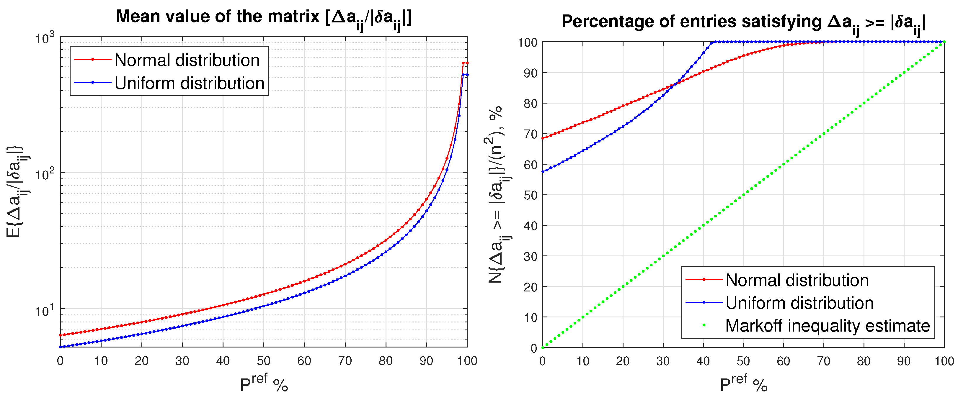
In Figure 1, we show the mean value of the matrix [ Δ a i j / | δ a i j | ] and the relative number N { Δ a i j | δ a i j | } / ( n 2 ) of the entries of the matrix | δ A | for which | δ a i j | | Δ a i j | , obtained for normal and uniform distribution of the entries of δ A and for different values of the desired probability, P r e f . For the case of normal distribution and P r e f = 90 % , the size of the probability entry bound, Δ a i j , decreases 10 times in comparison with the size of the entry bound δ A F , which allows the decrease of the mean value of the ratio Δ a i j / | δ a i j | from 638.38 to 63.838 (Table 1). For P r e f = 40 % , the probability bound, Δ a i j , is 60 times smaller than the bound δ A F , and even for this small desired probability the number of entries for which | δ a i j | | Δ a i j | is still 90.34 % .
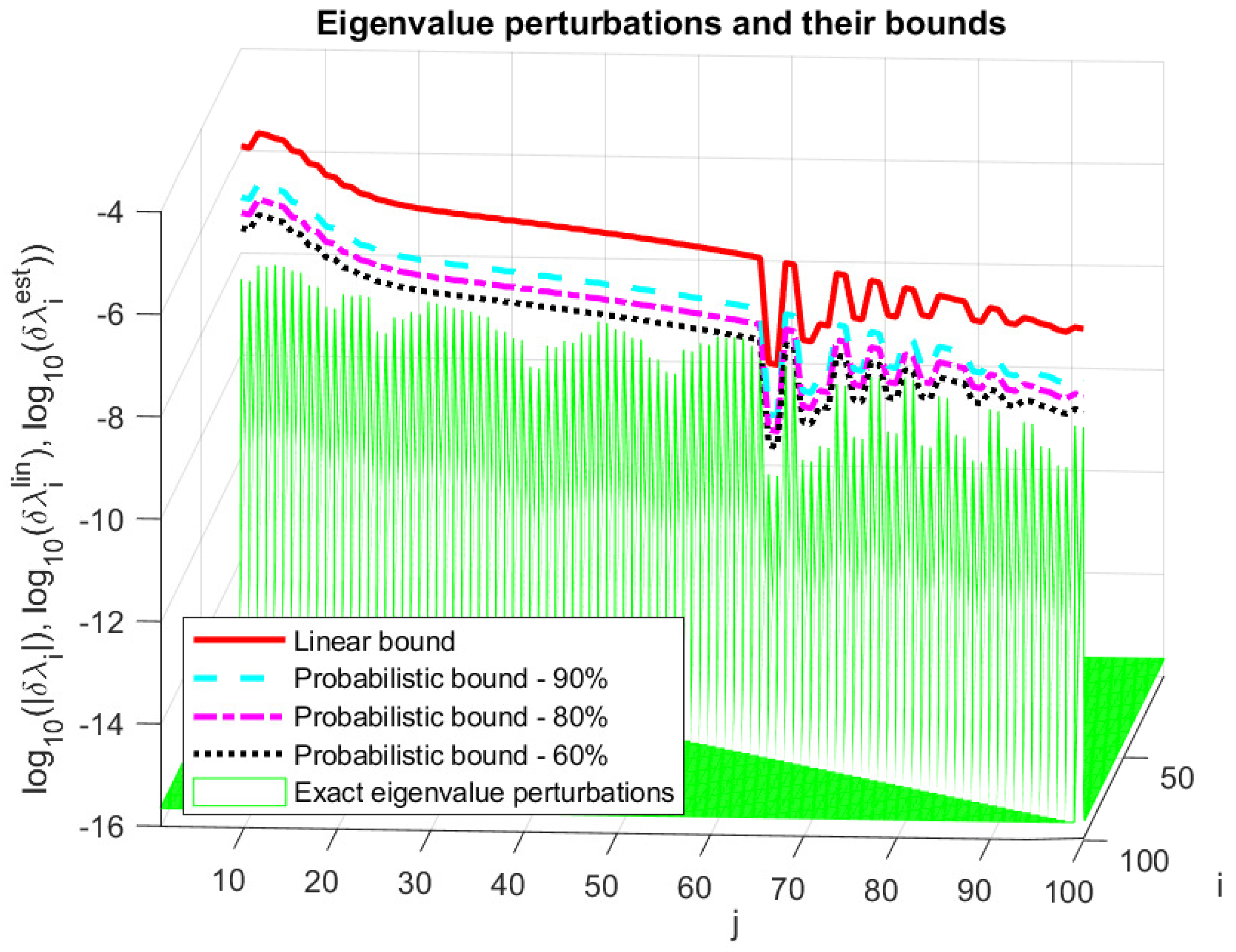
In Figure 2, we compare the asymptotic bound, δ λ i l i n , and the probabilistic estimate, δ λ i e s t , with the actual eigenvalue perturbations | δ λ i | for normal distribution of perturbation entries and probabilities P r e f = 90 % , 80 % and 60 % . (For clarity, the perturbations of the superdiagonal elements of T are hidden). The probabilistic bound, δ λ i e s t , is much tighter than the linear bound, δ λ i l i n , and the inequality | δ λ i | δ λ i e s t is satisfied for all eigenvalues and all chosen probabilities. In particular, the size of the estimate, δ λ i e s t , is 10 times smaller than the linear estimate, δ λ i l i n , for P r e f = 90 % , 20 times for P r e f = 80 % and 40 times for P r e f = 60 % .
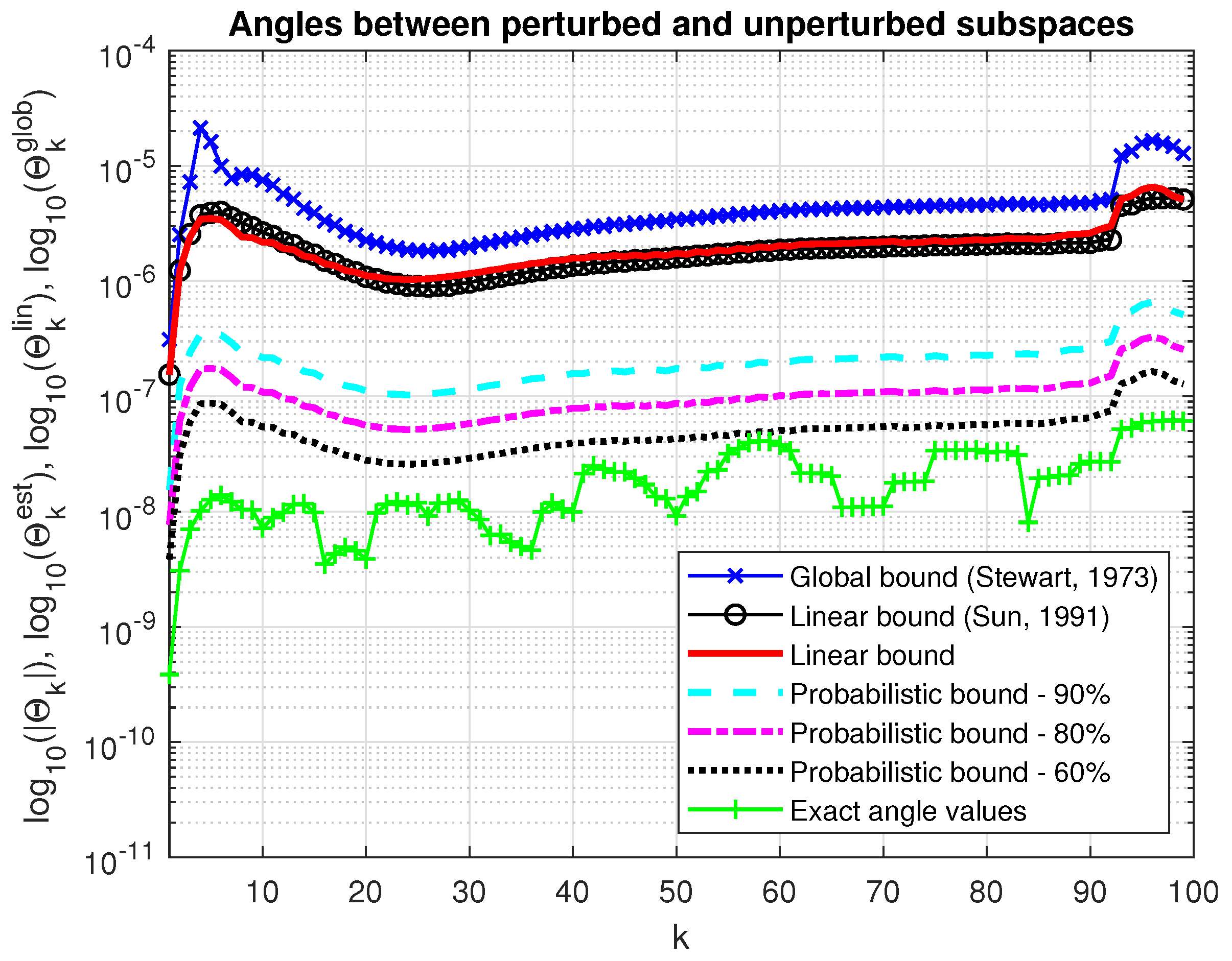
In Figure 3, we show the asymptotic bound, δ Θ k l i n , and the probabilistic estimate, δ Θ k e s t , along with the actual value | δ Θ k | of the maximum angle between the perturbed and unperturbed invariant subspace of dimensions k = 1 , 2 , , n 1 for the same probabilities P r e f = 90 % , 80 % and 60 % . The probability estimate satisfies | δ Θ k | < δ Θ k e s t for all 1 k < 100 . For comparison, we give the global bound on the maximum angle between the perturbed and unperturbed invariant subspaces computed by (20) and the first-order bound determined by (24). (The computation of the s e p -based estimate is performed by using the numerical algorithm, presented in [14].) The global bound is slightly larger than the asymptotic bounds, and the asymptotic bounds (24) and (34) coincide.

4. Perturbation Bounds for Deflating Subspaces

4.1. Problem Statement

Let A λ B be a square matrix pencil [35]. Then there exist unitary matrices U and V, such that T = U H A V and R = U H B V are both upper triangular. The pair ( T , R ) constitute the generalized Schur form of the pair ( A , B ) . The eigenvalues of A λ B are then equal to t i i / r i i , the ratios of the diagonal entries of T and R. Further on, we consider the case of regular pencils for which det ( A λ B ) 0 and in addition the matrix B is non-singular, i.e., the generalized eigenvalues are finite.
Suppose that the generalized Schur form of the pencil A λ B is reordered as
U H A V = T 11 T 12 0 T 22 , U H B V = R 11 R 12 0 R 22 ,
where T 11 λ R 11 contains k specified eigenvalues. Partitioning conformally the unitary matrices of the equivalence transformation as U = [ U 1 , U 2 ] , V = [ V 1 , V 2 ] , we obtain orthonormal bases U 1 C n × k and V 1 C n × k of the left, Y , and right, X , deflating subspace, respectively. The deflating subspaces satisfy the relations A X Y and B X Y .
Further on, we are interested in the sensitivity of the deflating subspaces corresponding to specified generalized eigenvalues of the pair ( T 11 , R 11 ) . Suppose that the matrices of the pencil A λ B are perturbed as A ˜ = A + δ A and B ˜ = B + δ B . The upper triangular matrices in the generalized Schur decomposition are represented as
U ˜ H A ˜ V ˜ = T ˜ 11 T ˜ 12 0 T ˜ 22 , U ˜ H B ˜ V ˜ = R ˜ 11 R ˜ 12 0 R ˜ 22 ,
where
U ˜ = U ˜ 1 , U ˜ 2 , V ˜ = V ˜ 1 , V ˜ 2
are the modified equivalence transformation matrices.

4.2. d i f -Based Global Bound

Let the unperturbed left and right deflation subspaces corresponding to the first k eigenvalues be denoted by Y = R ( U 1 ) and X = R ( V 1 ) , respectively, and their perturbed counterparts as X ˜ and Y ˜ .
If δ A and δ B are small, we may expect that the spaces X ˜ and Y ˜ will be close to the spaces X and Y , respectively.
Define the matrices
E = U H δ A V = E 11 E 12 E 21 E 22 , F = U H δ B V = F 11 F 12 F 21 F 22
and
M = I k T 22 T 11 T I n k , I k R 22 R 11 T I n k .
Note that matrix M is invertible if and only if the pencils T 11 λ R 11 and T 22 λ R 22 have no eigenvalues in common.
Define the difference between the spectra of T 11 λ R 11 and T 22 λ R 22 as [15]
dif ( T 11 , R 11 ; T 22 , R 22 ) = min [ S , W ] 0 T 22 S W T 11 R 22 S W R 11 F [ S , W ] F .
It is possible to prove the relationship
dif ( T 11 , R 11 ; T 22 , R 22 ) = σ min ( M ) ,
so that
M 1 2 = 1 / dif ( T 11 , R 11 ; T 22 , R 22 ) .
Assume that the spectra of T 11 λ R 11 and T 22 λ R 22 are disjoint so that
dif ( T 11 , R 11 ; T 22 , R 22 ) > 0 .
The following theorem gives an estimate of the sensitivity of a deflating subspace of a regular pencil.
Theorem 7 
([1,15]). Let the regular pencil A λ B be represented as in (38). Given the perturbation ( E , F ) , set
γ = ( E 21 , F 21 ) F , η = ( T 12 + E 12 , R 12 + F 12 ) F , δ = dif ( T 11 , R 11 ; T 22 , R 22 ) max { E 11 F + E 22 F , F 11 F + F 22 F } .
If δ > 0 and
η γ δ 2 < 1 4 ,
there are matrices P and Q satisfying
( P , Q ) F 2 γ δ + δ 2 4 γ η ,
such that the columns of V ˜ 1 = V 1 + V 2 P and U ˜ 1 = U 1 + U 2 Q span right and left deflating subspaces for A + δ A λ ( B + δ B ) . Note that
( P , Q ) F = P F 2 + Q F 2 .
It is possible to show that Equation (39) bounds the tangents of the canonical angles between X ˜ and X or Y ˜ and Y , similarly to the ordinary eigenvalue problem. Specifically, we have that
max { Φ max ( X ˜ , X ) , Θ max ( Y ˜ , Y ) } arctan 2 γ δ + δ 2 4 γ η .
Theorem 7 can be considered as a generalization of Theorem 4 for the ordinary eigenvalue problem.

4.3. Perturbation Expansion Bound

Global perturbation bounds for deflating subspaces that produce individual perturbation bounds for each subspace in a pair of deflating subspaces are presented in [18].
Theorem 8. 
Let ( A , B ) be an n × n regular matrix pair represented as in (38), and let X = R ( V 1 ) and Y = R ( U 1 ) . Moreover, let κ X , κ Y be defined by
κ X = P X 2 , κ Y = P Y 2 ,
where
P X = [ ( R 11 T I n k ) S 1 , ( T 11 T I n k ) S 1 ] , P Y = [ ( I k R 22 ) S 1 , ( I k T 22 ) S 1 ] , S = T 11 R 22 R 11 T T 22
and let
κ = κ X 2 + κ Y 2 , γ = E 21 F 21 F , η = T 12 + E 12 R 12 + F 12 F ,
ε = ( E 11 , F 11 ) F 2 + ( E 22 , F 22 ) F 2 .
If
κ ( 2 γ η + ε ) < 1 ,
then there exists a pair X ˜ = R ( V ˜ 1 ) and Y ˜ = R ( U ˜ 1 ) of k-dimensional deflating subspaces of ( A + δ A , B + δ B ) such that
Φ max ( X ˜ , X ) arctan 2 κ X γ 1 κ ε + ( 1 κ ε ) 2 4 κ 2 γ η ,
Θ max ( X ˜ , X ) arctan 2 κ Y γ 1 κ ε + ( 1 κ ε ) 2 4 κ 2 γ η .

4.4. Bound by the Splitting Operator Method

The application of the splitting operator method to the perturbation analysis of the generalized Schur decomposition is performed in [34].
Consider again the generalized Schur decomposition (38). To derive perturbation bounds of the matrices δ U 1 = U ˜ 1 U 1 and δ V 1 = V ˜ 1 V 1 , we introduce the perturbation parameter vectors
x = vec ( Low ( δ W U ) ) C p , p = n ( n 1 ) / 2 ,
and
y = vec ( Low ( δ W V ) ) C p ,
where δ W U = U H δ U and δ W V = V H δ V . Let
F = U H ( δ A ) V , G = U H ( δ B ) V
and construct the vectors
f = vec ( Low ( F ) ) C p , g = vec ( Low ( G ) ) C p .
Then, asymptotic bounds of x and y can be found by solving the linear system of equations
M x f M x g M y f M y g x y = f g ,
where
M x f = Ω ( T T I n ) Ω T , M x g = Ω ( I n T ) Ω T ,
M y f = Ω ( R T I n ) Ω T , M y g = Ω ( I n R ) Ω T
and
Ω : = diag ( Ω 1 , Ω 2 , , Ω n 1 ) , 0 p × n R p × n 2 , Ω k : = 0 ( n k ) × k , I n k R ( n k ) × n , k = 1 , 2 , , n 1 .
Hence, linear approximations of the elements of x and y can be determined from
x l i n = M , 1 : 2 p 1 2 δ A F 2 + δ B F 2 ,
y l i n = M + p , 1 : 2 p 1 2 δ A F 2 + δ B F 2 ,
= 1 , 2 , , p ,
where
M = M x f M x g M y f M y g .
The matrices | δ W U | and | δ W V | can be estimated as
| δ W U | δ W U l i n + Δ W U ,
| δ W V | δ W V l i n + Δ W V ,
where
δ W U l i n = 0 x 1 l i n x 2 l i n x n 1 l i n x 1 l i n 0 x n l i n x 2 n 3 l i n x 2 x n l i n 0 x 3 n 6 l i n x n 1 l i n x 2 n 3 l i n x 3 n 6 l i n 0 R n × n ,
δ W V l i n = 0 y 1 l i n y 2 l i n y n 1 l i n y 1 l i n 0 y n l i n y 2 n 3 l i n y 2 y n l i n 0 y 3 n 6 l i n y n 1 l i n y 2 n 3 l i n y 3 n 6 l i n 0 R n × n
and Δ W U , Δ W V contain higher-order terms in x , y . Thus, asymptotic approximation of the matrices | δ U | and | δ V | can be determined as
| δ U | δ U l i n = | U | | U H δ U | = | U | δ W U l i n ,
| δ V | δ V l i n = | V | | V H δ V | = | V | δ W V l i n .
Let V ˜ 1 and V 1 be the orthonormal bases of the perturbed and unperturbed right deflation subspace, X , of dimension k, and U ˜ 1 and U 1 be, respectively, the orthonormal bases of the perturbed and unperturbed left deflation subspace, Y , of the same dimension. Since
V ˜ 1 = V 1 + δ V 1 , V 2 H V 1 = 0 , U ˜ 1 = U 1 + δ U 1 , U 2 H U 1 = 0 ,
we have that
sin ( Φ max ( X ˜ , X ) ) = V 2 H δ V 1 2 , sin ( Θ max ( Y ˜ , Y ) ) = U 2 H δ U 1 2 .
Using these expressions, it is possible to show that
Φ max ( X ˜ , X ) = arcsin ( δ W V k + 1 : n , 1 : k p 2 ) , Θ max ( Y ˜ , Y ) = arcsin ( δ W U k + 1 : n , 1 : k p 2 ) .
Implementing the asymptotic approximations of the elements of the vectors x and y, we obtain the following result.
Theorem 9. 
Let the pair ( A , B ) be decomposed, as in (38), and assume that the Frobenius norms of the perturbations δ A and δ B are known. Set
L X = M 1 + p , 1 : 2 p 1 M 2 + p , 1 : 2 p 1 M n + p , 1 : 2 p 1 M n 1 + p , 1 : 2 p 1 M 2 n 3 + p , 1 : 2 p 1 M 3 n 6 + p , 1 : 2 p 1 C n × 2 n p ,
L Y = M 1 , 1 : 2 p 1 M 2 , 1 : 2 p 1 M n , 1 : 2 p 1 M n 1 , 1 : 2 p 1 M 2 n 3 , 1 : 2 p 1 M 3 n 6 , 1 : 2 p 1 C n × 2 n p .
Then, the following asymptotic bounds of the angles between the perturbed and unperturbed deflation subspaces of dimension 1 k < n are valid,
Φ max l i n ( X ˜ , X ) = arcsin L X k + 1 : p , 1 : 2 k p 2 δ A F 2 + δ B F 2 ,
Θ max l i n ( Y ˜ , Y ) = arcsin L Y k + 1 : p , 1 : 2 k p 2 δ A F 2 + δ B F 2 .
Consider the sensitivity of the generalized eigenvalues, i.e., the sensitivity of a simple finite generalized eigenvalue, λ i , under perturbations of the matrices A and B. If the perturbed pencil is denoted by
A ˜ + λ ˜ B ˜ = A + δ A + λ ˜ ( B + δ B ) ,
we want to know how the difference between λ ˜ and λ depends on the size of the perturbation measured by the quantity
ε = δ A F 2 + δ B F 2 .
The distance between two generalized eigenvalues λ = α / β and μ = γ / δ is measured by the so-called chordal distance, defined as [15]
χ ( λ , μ ) = | α δ β γ | | α | 2 + | β | 2 | γ | 2 + | δ | 2 .
Substituting
α = t i i , α ˜ = t ˜ i i , β = r i i , β ˜ = r ˜ i i ,
we find that
χ ( λ , λ ˜ ) = | t i i r ˜ i i r i i t ˜ i i | | t i i | 2 + | r i i | 2 | t ˜ i i | 2 + | r ˜ i i | 2
or, in a first order-approximation,
χ l i n ( λ , λ ˜ ) = | r i i δ t i i + t i i δ r i i | | t i i | 2 + | r i i | 2
The asymptotic approximations of the diagonal element perturbations of the matrices R and T satisfy
δ t i i = cond ( t i i ) δ A F 2 + δ B F 2 ,
δ r i i = cond ( r i i ) δ A F 2 + δ B F 2 ,
where the numbers cond ( t i i ) and cond ( r i i ) are determined from
cond ( t i i ) = Z i , 1 : 2 n 2 , cond ( r i i ) = Z i + n , 1 : 2 n 2 ,
Z = [ Q M 1 , I 2 n ] , Q = N a 1 N a 2 N b 1 N b 2 ,
N a 1 = Π ( T T I n ) Ω T , N a 2 = Π ( I n T ) Ω T , N b 1 = Π ( R T I n ) Ω T , N b 2 = Π ( I n R ) Ω T .
Replacing the expressions for the perturbations δ t i i and δ r i i in (58), we find that
χ ( λ ˜ , λ ) χ l i n ( λ ˜ , λ ) = cond ( λ i ) δ A F 2 + δ B F 2
where the number
cond ( λ i ) = | r i i | cond ( t i i ) + | t i i | cond ( r i i ) | t i i | 2 + | r i i | 2
can be considered as a condition number of the generalized eigenvalue, λ i .

4.5. Probabilistic Perturbation Bound

Implementing again Theorem 3, the probabilistic perturbation bounds of the perturbation parameter vectors x and y can be found from (49) and (50), respectively, replacing the quantity δ A F 2 + δ B F 2 by the ratio δ A F 2 + δ B F 2 / Ξ , where Ξ is determined according to (3) from the desired probability, P r e f , and the problem order, n. This means that the probabilistic asymptotic estimates of | δ U | and | δ V | can be obtained from (54) and (55), replacing the linear estimates x l i n , y l i n by
x e s t = x l i n / Ξ , y e s t = y l i n / Ξ ,
respectively. As a result, we obtain the probabilistic bounds on the angles between the perturbed and unperturbed deflating subspaces as
Φ max e s t ( X ˜ , X ) = arcsin L X k + 1 : p , 1 : 2 k p 2 δ A F 2 + δ B F 2 / Ξ ,
Θ max e s t ( Y ˜ , Y ) = arcsin L Y k + 1 : p , 1 : 2 k p 2 δ A F 2 + δ B F 2 / Ξ , k = 1 , 2 , , n 1 .
In the same way, we may obtain a probabilistic asymptotic estimate of the eigenvalue perturbations, replacing in (61) the expression δ A F 2 + δ B F 2 by
δ A F 2 + δ B F 2 / Ξ . This yields
χ ( λ ˜ , λ ) χ e s t ( λ ˜ , λ ) = cond ( λ i ) δ A F 2 + δ B F 2 / Ξ .

4.6. Bound Comparison

Example 2. 
Consider a 80 × 80 matrix pencil A λ B , where
A = Q A J A Q A 1 , B = Q B J B Q B 1 ,
J A = 0.1 0.1 τ τ τ τ 0.1 0.1 τ τ τ τ 0.2 0.2 τ τ 0.2 0.2 τ τ 5.0 5.0 5.0 5.0 , J B = 1 ρ ρ ρ ρ ρ 1 ρ ρ ρ ρ 1 ρ ρ ρ 1 ρ ρ 1 ρ 1 , τ = 0.05 , ρ = 0.1 ,
the matrices Q A and Q B are constructed as in Example 1,
Q A = H 2 Σ A H 1 , Q B = H 2 Σ B H 1 , H 1 = I n 2 u u T / n , H 2 = I n 2 v v T / n , u = [ 1 , 1 , 1 , , 1 ] T , v = [ 1 , 1 , 1 , , ( 1 ) n 1 ] T , Σ A = diag ( 1 , σ A , σ A 2 , , σ A n 1 ) , Σ B = diag ( 1 , σ B , σ B 2 , , σ B n 1 ) ,
H 1 , H 2 are elementary reflections, σ A is taken equal to 1.02 and σ B is taken equal to 1.01 .
In Figure 4, we give the mean value of the ratios Δ a i j / | δ a i j | and Δ b i j / | δ b i j | obtained for two random distributions and different values of P r e f between 100% and 0%, where Δ A is the probabilistic bound of | δ A | and Δ B is the probabilistic bound of | δ B | . For each P r e f , the scaling factor, Ξ, is determined from (3). The same ratios are represented numerically in Table 2 for the perturbation with normal distribution and three values of P r e f . The results show that if, instead of the deterministic estimates of δ A and δ B , we use the corresponding probabilistic estimates Δ A and Δ B with P r e f = 90 %, then the mean values of [ Δ a i j / | δ a i j | ] and [ Δ b i j / | δ b i j | ] decrease by a factor of eight. A further reduction in P r e f to 80 % leads to the decreasing of the mean values by a factor of 16.
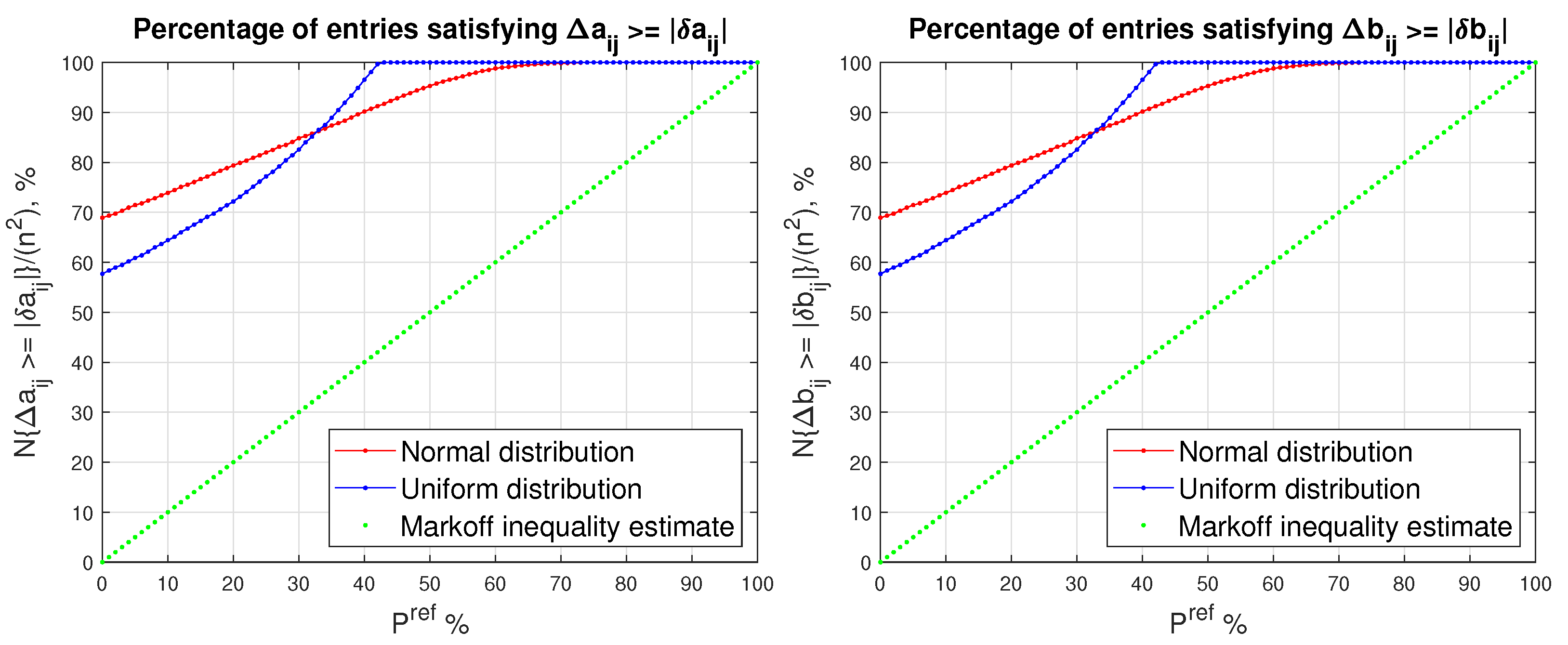
In Figure 5, we show the relative numbers N { Δ a i j | δ a i j | } / ( n 2 ) and N { Δ b i j | δ b i j | } / ( n 2 ) of the entries for which Δ a i j | δ a i j | and Δ b i j | δ b i j | , respectively. In both cases, the relative number of entries for which Δ a i j | δ a i j | and Δ b i j | δ b i j | remains 100 %, which shows that the decreasing of the estimates of δ A and δ B can be done safely.
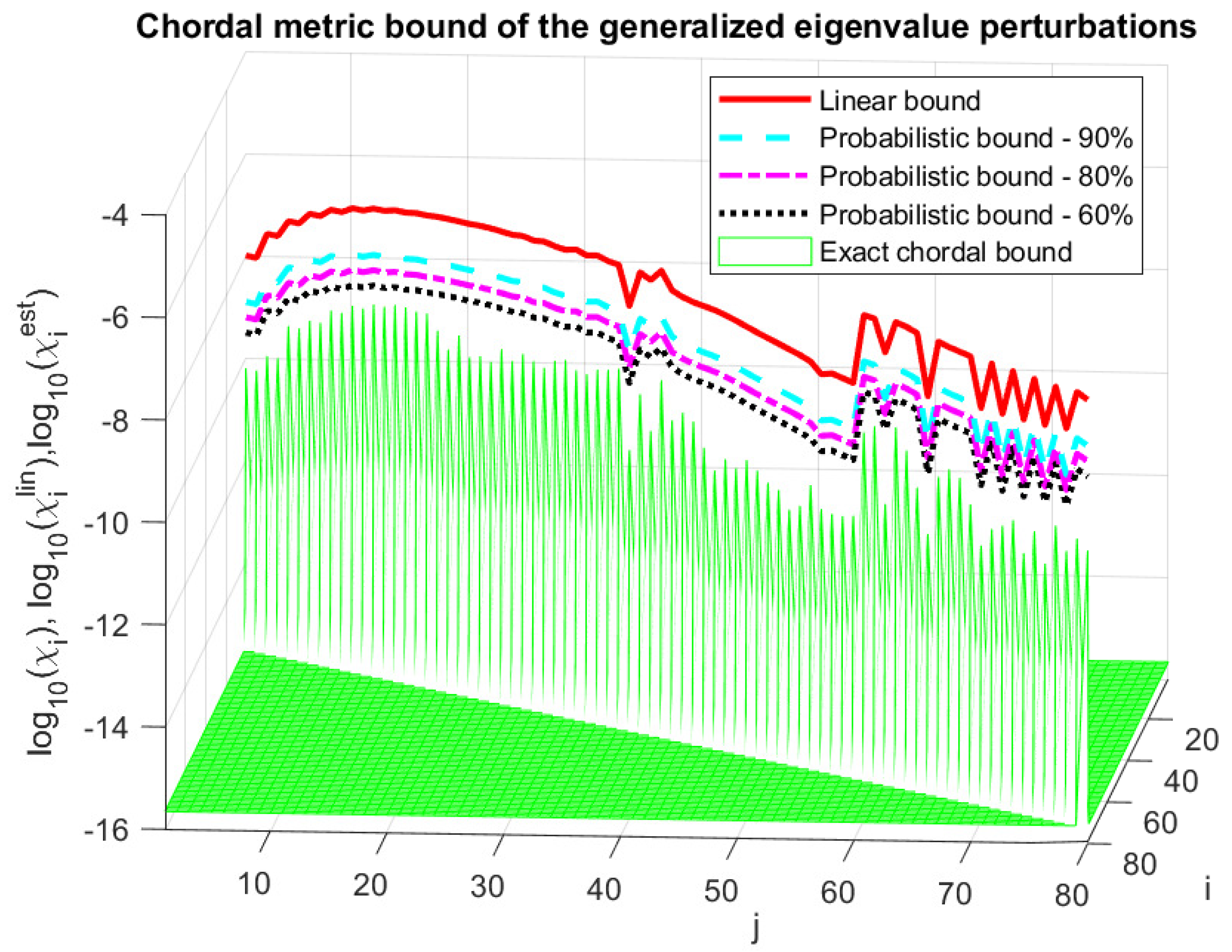
In Figure 6, we show the asymptotic chordal metric bound, χ i l i n , of the generalized eigenvalue perturbations along with the probabilistic estimates, χ i e s t , and the actual eigenvalue perturbations | χ i | for normal distribution of perturbation entries and probabilities P r e f = 90 % , 80 % and 60 % . The probabilistic bound, χ i e s t , is much tighter than the linear bound, χ i l i n , and the inequality | χ i | χ i e s t is satisfied for all eigenvalues. In particular, the size of the estimate, χ i e s t , is 8 times smaller than the linear estimate, χ i l i n , for P r e f = 90 % , 16 times for P r e f = 80 % and 32 times for P r e f = 60 % .
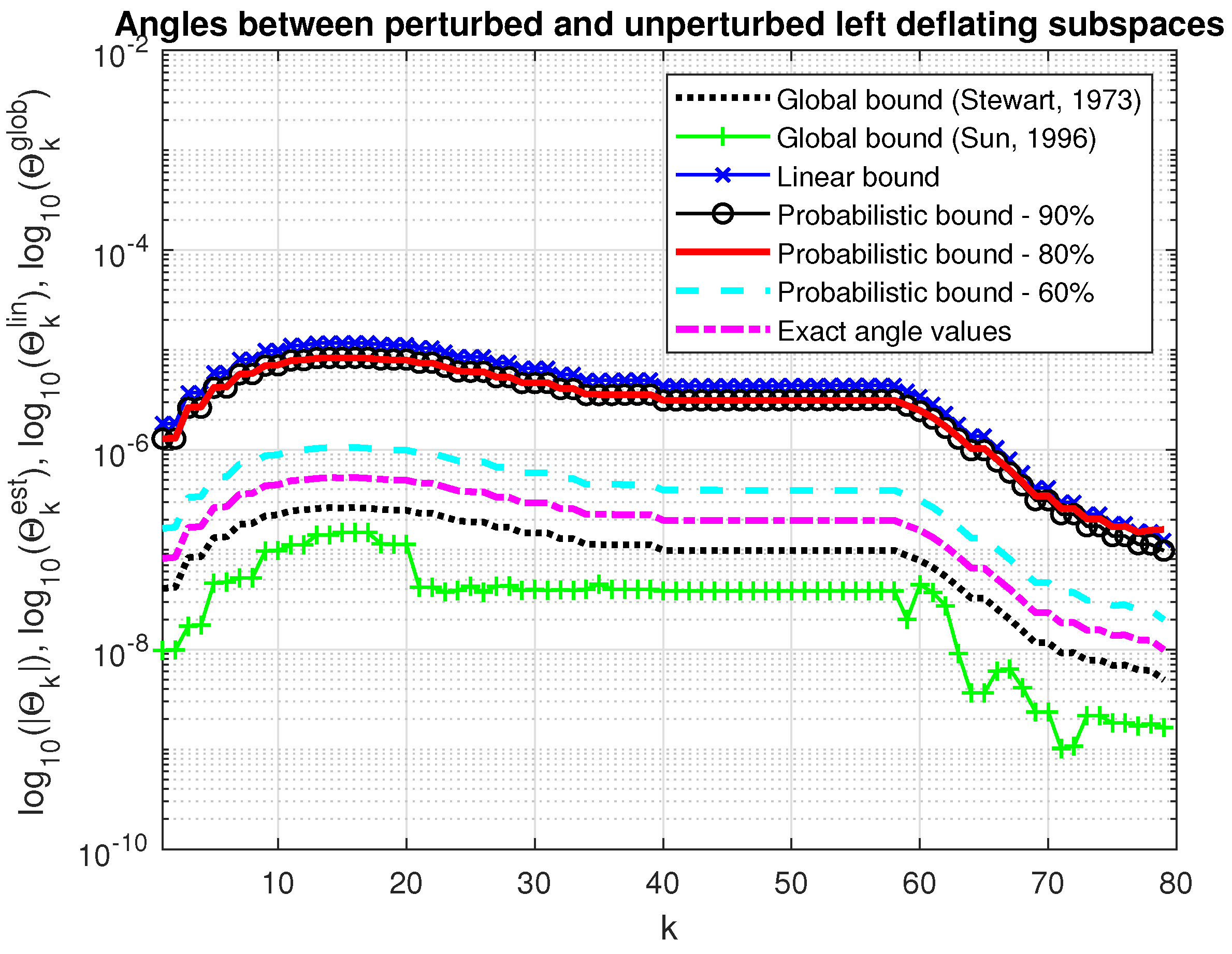
In Figure 7 and Figure 8, we show the asymptotic bounds, δ Φ k l i n and δ Θ k l i n , of the maximum angles between the perturbed and unperturbed deflating subspaces of dimension k = 1 , 2 , , n 1 along with the probabilistic estimates, δ Φ k e s t , δ Θ k e s t , and the actual values of these angles for the same probabilities P r e f = 90 % , 80 % and 60 % . The probability estimates satisfy | δ Φ k | < δ Φ k e s t , | δ Θ k | < δ Θ k e s t for all 1 k < 100 . For comparison, we give also the global bounds on the maximum angles between the perturbed and unperturbed invariant subspaces computed by (40) and (43), (44). Since the determination of the corresponding bounds requires us to know the norms of parts of the perturbations E and F, which are unknown, these norms are replaced by the Frobenius norms of the whole corresponding matrices. The global bounds practically coincide with the corresponding asymptotic bounds obtained by the splitting operator method.

5. Perturbation Bounds for Singular Subspaces

5.1. Problem Statement

Let A R m × n . The factorization
U H A V = Σ ,
where U R m × m , V R n × n are orthogonal matrices and Σ is a diagonal matrix, is called the singular value decomposition of A ([38], Section 2.6). If m n , matrix Σ has the form
Σ = Σ n 0 ( m n ) × n ) , Σ n = diag σ 1 , σ 2 , , σ n .
where the numbers σ i 0 are the singular values of A. If U = [ U 1 , U 2 ] and [ V 1 , V 2 ] are partitioned such that U 1 R m × k , V 1 R n × k , k < n , then X = R ( V 1 ) , Y = R ( U 1 ) form a pair of singular subspaces for A. These subspaces satisfy A X Y and A T Y X .
If matrix A is subject to a perturbation, δ A , then there exists another pair of orthogonal matrices, U ˜ = [ U ˜ 1 , U ˜ 2 ] , V ˜ = [ V ˜ 1 , V ˜ 2 ] , and a diagonal matrix, Σ ˜ , such that
U ˜ H ( A + δ A ) V ˜ = Σ ˜
where
Σ ˜ = Σ ˜ n 0 ( m n ) × n ) , Σ ˜ n = diag σ ˜ 1 , σ ˜ 2 , , σ ˜ n , Σ ˜ n = Σ n + δ Σ n , δ Σ n = diag δ σ 1 , δ σ 2 , , δ σ n .
The aim of the perturbation analysis of singular subspaces consists in bounding the angles between the perturbed, X ˜ = R ( V ˜ 1 ) , and unperturbed, X = R ( V 1 ) , right singular subspaces, and the angles between the perturbed, Y ˜ = R ( U ˜ 1 ) , and unperturbed, Y = R ( U 1 ) , left singular subspaces.

5.2. Global Bound

Consider first the global perturbation bound on the singular subspaces derived by Stewart [16].
Theorem 10. 
Let matrix A be decomposed, as in (65), and let X and Y form a pair of singular subspaces for A. Let δ A R m × n be given and partition U T Δ A V conformingly with U and V as
E = U T δ A V = E 11 E 12 E 21 E 22 , E 11 C k × k .
Let
η = γ = ( E 21 , E 12 T ) F
and let
δ = min 1 j < k k + 1 q m | σ j σ q | E 11 2 E 22 2 ,
where, if m n , Σ is understood to have m n zero singular values. Set
κ = 2 k 2 1 2 k 2 + 1 4 k 2 , k 2 = γ η δ .
If
γ δ < 1 2 ,
then there are matrices P R ( m k ) × k and Q R ( n k ) × k satisfying
( P , Q ) F ( 1 + κ ) γ δ < 2 γ δ
such that X ˜ = R ( V 1 + V 2 P ) and Y ˜ = R ( U 1 + U 2 Q ) form a pair of singular subspaces of A + Δ A .
Theorem 10 bounds the tangents of the angles between the perturbed, X ˜ , and unperturbed, X , right singular subspaces and the angles between the perturbed, Y ˜ , and unperturbed, Y , left singular subspaces of A. Thus, the maximum angles between perturbed and unperturbed singular subspaces fulfil
Φ max ( X ˜ , X ) arctan ( 1 + κ ) γ δ ,
Θ max ( Y ˜ , Y ) arctan ( 1 + κ ) γ δ .
Note that Theorem 10 produces equal bounds on the maximum angles between the perturbed and unperturbed right and left singular subspaces.

5.3. Perturbation Expansion Bound

Global perturbation bounds for singular subspaces that produce individual perturbation bounds for each subspace in a pair of singular subspaces are presented in [18].
Theorem 11. 
Let A R m × n ( m n ) and let U = [ U 1 , U 2 ] R m × m , V = [ V 1 , V 2 ] R n × n be orthogonal matrices with U 1 R m × k , V 1 R n × k such that
U H A V = Σ 1 0 0 Σ 2 ,
Σ 1 = diag ( σ 1 , , σ k ) , Σ 2 = Σ 21 0 , Σ 21 = diag ( σ k + 1 , , σ n ) .
Assume that σ j 0 for each j and the singular values of Σ 1 are different from the singular values of Σ 2 . Let X = R ( V 1 ) and Y = R ( U 1 ) . For δ A R m × n , let
E = U T δ A V = E 11 E 12 E 21 E 22 , E 11 R k × k .
Moreover, let
κ X = max 1 j < k k + 1 q n σ j 2 + σ q 2 | σ j 2 σ q 2 | , κ Y = max 1 j < k k + 1 q m σ j 2 + σ q 2 | σ j 2 σ q 2 | ,
where we define σ n + 1 = = σ m = 0 if m > n and let
κ = κ X 2 + κ Y 2 , γ = E 12 T F 21 F , ε = E 11 2 + E 22 2 .
If
κ ( 2 γ + ε ) < 1 ,
then there exists a pair, X ˜ = R ( V ˜ 1 ) and Y ˜ = R ( U ˜ 1 ) , of k-dimensional singular subspaces of A + δ A , such that
Φ max ( X ˜ , X ) arctan 2 κ X γ 1 κ ε + ( 1 κ ε ) 2 4 κ 2 γ 2 ,
Θ max ( Y ˜ , Y ) arctan 2 κ Y γ 1 κ ε + ( 1 κ ε ) 2 4 κ 2 γ 2 .

5.4. Bound by the Splitting Operator Method

Similarly to the perturbation analysis of the generalized Schur decomposition, performed by using the splitting operator method, it is appropriate first to find bounds on the entries of the matrices δ W U : = U T δ U n and δ W V : = V T δ V , where U n is a matrix that consists of the first n columns of U. The matrices δ W U and δ W V are related to the corresponding perturbations δ U n = U δ W U and δ V = V δ W V by orthogonal transformations.
Let us define the vectors of the subdiagonal entries of the matrices δ W U and δ W V ,
x = vec ( Low ( δ W U ) ) , y = vec ( Low ( δ W V ) ) .
We have that
x = [ u 2 T δ u 1 , u 3 T δ u 1 , , u m T δ u 1 m 1 , u 3 T δ u 2 , , u m T δ u 2 m 2 , , u n + 1 T δ u n , , u m T δ u n m n ] T , : = [ x 1 , x 2 , , x p ] T R p , y : = [ v 2 T δ v 1 , v 3 T δ v 1 , , v n T δ v 1 n 1 , v 3 T δ v 2 , , v n T δ v 2 n 2 , , v n T δ v n 1 1 ] T , : = [ y 1 , y 2 , , y q ] T R q ,
where
p = i = 1 n ( m i ) = n ( n 1 ) / 2 + ( m n ) n = n ( 2 m n 1 ) / 2 , q = n ( n 1 ) / 2 .
It is fulfilled that
x k = u i T δ u j , k = i + ( j 1 ) m j ( j + 1 ) 2 , 1 j n , j < i m , 1 k p , y = v i T δ v j , = i + ( j 1 ) n j ( j + 1 ) 2 , 1 j n , j < i n 1 , 1 q .
Further on the quantities x k , k = 1 , 2 , , p and y , = 1 , 2 , , q will be considered as perturbation parameters since they determine the perturbations δ U 1 and δ V of the singular vectors.
Let us represent the matrix δ E = U T δ A V as
δ E = δ E 1 δ E 2 , δ E 1 R n × n , δ E 2 R ( m n ) × n .
Define the vectors
x ( 1 ) = Ω 1 x , a n d x ( 2 ) = Ω 2 x ,
where
Ω 1 : = diag ( ω 1 , ω 2 , , ω n ) R q × p , ω k : = I n k , 0 ( n k ) | × ( m n ) R ( n k ) × ( m k ) , k = 1 , 2 , , n , Ω 1 Ω 1 T = I q , Ω 1 2 = 1 , Ω 2 : = diag ( ω 1 , ω 2 , , ω n ) R ( m n ) n × p , ω k : = 0 ( m n ) × ( n k ) , I m n R ( m n ) × ( m k ) , k = 1 , 2 , , n , Ω 2 Ω 2 T = I ( m n ) n , Ω 2 2 = 1 .
It is possible to show that
x = Ω 1 T x ( 1 ) + Ω 2 T x ( 2 ) .
Following the analysis performed in [30], it can be shown that the unknown vectors x ( 1 ) and y satisfy the system of linear equations
S 1 S 2 S 2 S 1 x ( 1 ) y = f g + Δ 1 Δ 2 .
where
S 1 = diag ( σ 1 , σ 1 , , σ 1 n 1 , σ 2 , , σ 2 n 2 , , σ n 1 1 ) ,
S 2 = diag ( σ 2 , σ 3 , , σ n n 1 , σ 3 , , σ n n 2 , , σ n 1 ) , S i R q × q , i = 1 , 2 ,
f = vec ( Low ( δ E 1 ) ) R q , g = vec ( ( Up ( δ E 1 ) ) T ) R q ,
and Δ 1 , Δ 2 contain higher-order terms in δ U n , δ A and δ V .
In this way, the determining of the vectors x ( 1 ) and y reduces to the solution of the system of symmetric coupled equations (75) with diagonal matrices of size q × q . The vector x ( 2 ) can be found from the separate equation
x ( 2 ) = vec ( ( δ E 2 + Δ 3 ) Σ n 1 ) ,
where Δ 3 contains higher-order terms in δ u j , δ v j , δ A and Σ n , defined in (66).
Neglecting the higher-order terms Δ 1 , Δ 2 in (75), we obtain
x ( 1 ) y = S x f S x g S y f S y g f g ,
where, taking into account that S 1 and S 2 commute, we have that
S x f = ( S 2 2 S 1 2 ) 1 S 1 R q × q , S y g = S x f , S x g = ( S 2 2 S 1 2 ) 1 S 2 R q × q , S y f = S x g .
The matrices S x f and S x g are diagonal matrices whose nontrivial entries are determined by the singular values σ 1 , , σ n .
Hence, the components of the vectors x ( 1 ) and y satisfy
| x ( 1 ) | S x f , 1 : q , S x g , 1 : q 2 f g 2 , | y | S y f , 1 : q , S y g , 1 : q 2 f g 2 , = 1 , 2 , , q .
Taking into account the diagonal form of S x f , S x g , S y f , S y g , we obtain that
| x ( 1 ) | | S x f , | | f | + | S x g , | | g | ,
| y | | S y f , | | f | + | S y g , | | g | , = 1 , 2 , , q .
Since only one element of f and g participates in (79) and (80), these elements can be replaced by δ A 2 , and we find that the linear approximations of the vectors x ( 1 ) and y fulfil
| x ( 1 ) | x ( 1 ) l i n , | y | y l i n ,
x ( 1 ) l i n = ( | S x f , | + | S x g , | ) δ A 2 ,
y l i n = ( | S y f , | + | S y g , | ) δ A 2 , = 1 , 2 , , q .
where S y g = S x f , S y f = S x g .
An asymptotic estimate of the vector x ( 2 ) is obtained from (78), neglecting the higher-order term Δ 3 . Since each element of x ( 2 ) depends only on one element of δ E 2 , we have that
x ( 2 ) l i n = vec ( Z ) , Z = δ A 2 × 1 / σ 1 1 / σ 2 1 / σ n 1 / σ 1 1 / σ 2 1 / σ n 1 / σ 1 1 / σ 2 1 / σ n .
As a result of determining the linear estimates (82)–(84), we obtain an asymptotic approximation of the vector x as
| x | x l i n ,
where
x l i n = Ω 1 T x ( 1 ) l i n + Ω 2 T x ( 2 ) l i n .
The matrices | δ W U | and | δ W V | can be estimated as
| δ W U | δ W U l i n + Δ W U ,
| δ W V | δ W V l i n + Δ W V ,
where
δ W U l i n = 0 x 1 l i n x 2 l i n x n 1 l i n x 1 l i n 0 x m l i n x m + n 3 l i n x 2 l i n x m l i n 0 x 2 m + n 6 l i n x n 1 l i n x m + n 3 l i n x 2 m + n 6 l i n 0 x n l i n x m + n 2 l i n x 2 m + n 5 l i n x ( n 1 ) ( 2 m n ) / 2 + 1 l i n x m 1 l i n x 2 m 3 l i n x 3 m 6 l i n x p l i n ,
δ W V l i n = 0 y 1 l i n y 2 l i n y n 1 l i n y 1 l i n 0 y n l i n y 2 n 3 l i n y 2 l i n y n l i n 0 y 3 n 6 l i n y n 1 l i n y 2 n 3 l i n y 3 n 6 l i n 0
and the matrices Δ W U , Δ W V contain higher-order terms in δ U , δ V . The matrices δ W U l i n and δ W V l i n are asymptotic approximations of the matrices δ W U and δ W V , respectively.
We have that
| δ U n | | U | | U T δ U n | δ U n l i n = | U | δ W U l i n ,
| δ V | | V | | V T δ V | δ V l i n = | V | δ W V l i n ,
Assume that the singular value decomposition of A is reordered as
U T A V = Σ 1 0 0 Σ 2 ,
where U = [ U 1 , U 2 ] and V = [ V 1 , V 2 ] are orthogonal matrices with U 1 R m × k and V 1 R n × k , k < n , and Σ 1 R k × k contains the desired singular values. The matrices U ˜ 1 and U 1 are the orthonormal bases of the perturbed and unperturbed left singular subspace, X , of dimension k < n , and V ˜ 1 and V 1 are the orthonormal bases of the perturbed and unperturbed right deflation subspace, Y , of the same dimension. We have that
sin ( Φ max ( X ˜ , X ) ) = V 2 T δ V 1 2 = V 1 : n , k + 1 : n T δ V 1 : n , 1 : k 2 , sin ( Θ max ( Y ˜ , Y ) ) = U 2 T δ U 1 2 = U 1 : m , k + 1 : m T δ U 1 : m , 1 : k 2 , k = 1 , , n 1 .
Using the asymptotic approximations of the elements of the vectors x and y, we obtain the following result.
Theorem 12. 
Let matrix A be decomposed, as in (92). Given the spectral norm of the perturbation δ A , set the matrices δ W U l i n and δ W V l i n in (88), (89) using the linear estimates of the perturbation parameters x and y determined from (81)–(84). Then, the asymptotic bounds of the angles between the perturbed and unperturbed singular subspaces of dimension k are given by
Φ max l i n ( X ˜ , X ) = arcsin ( δ W V l i n k + 1 : n , 1 : k 2 ) ,
Θ max l i n ( Y ˜ , Y ) = arcsin ( δ W U l i n k + 1 : m , 1 : k 2 ) , k = 1 , , n 1 .
The perturbed matrix of the singular values satisfies
δ Σ n = diag ( E ) + diag ( Δ 4 ) ,
where E = U T δ A V and Δ 4 contains higher-order terms in δ U , δ V and δ A . Neglecting the higher-order terms, we obtain for the singular value perturbation the asymptotic bound
| δ σ i | = | δ E i i | , i = 1 , 2 , , n .
Bounding each diagonal element | δ E i i | by δ A 2 , we find the normwise estimate
| δ σ i | δ A 2 ,
which is in accordance with Weyl’s theorem ([44], Chapter 1). We have in a first-order approximation that
| δ σ i | δ σ i l i n , δ σ i l i n : = δ A 2 , i = 1 , 2 , , n .

5.5. Probabilistic Perturbation Bound

Implementing a derivation similar to the one used in the proof of Theorem 3, the probabilistic estimates x e s t and y e s t of the parameter vectors x and y can be obtained from the deterministic estimates x l i n and y l i n . For this aim, the value of δ A 2 in the expressions (82) and (83) for x l i n and y l i n , respectively, is replaced by the value of δ A 2 / Ξ 2 , where Ξ 2 is determined from (4) for the specified value of P r e f . According to (85), the probabilistic perturbation bound of x fulfils
x e s t = Ω 1 T x ( 1 ) l i n / Ξ 2 + Ω 2 T x ( 2 ) l i n / Ξ 2 ,
where the estimates x ( 1 ) l i n and x ( 2 ) l i n satisfy (81) and (84), respectively. The bound of y is found from
y e s t = y l i n / Ξ 2 ,
where y l i n satisfies (83).
The bounds on | δ U n | and | δ V | are determined from (90) and (91), respectively. According to (96), the probability bound on the singular value perturbations is found from
δ σ i e s t = δ A 2 / Ξ 2 , i = 1 , 2 , , n .

5.6. Bound Comparison

Example 3. 
Consider a 400 × 200 matrix, taken as
A = U 0 Σ 0 0 ( m n ) × n V 0 T ,
where
Σ 0 = diag ( σ 0 1 , σ 0 2 , , σ 0 n ) , σ 0 i = ( n i + 1 ) / 30000 , i = 1 , 2 , , n ,
the matrices U 0 and V 0 are constructed as in Example 2,
U 0 = M 2 S U M 1 , M 1 = I m 2 e e T / m , M 2 = I m 2 f f T / m , e = [ 1 , 1 , 1 , , 1 ] T , f = [ 1 , 1 , 1 , , ( 1 ) m 1 ] T , S U = diag ( 1 , σ , σ 2 , , σ m 1 ) , V 0 = N 2 S V N 1 , N 1 = I n 2 g g T / n , N 2 = I n 2 h h T / n , g = [ 1 , 1 , 1 , , 1 ] T , h = [ 1 , 1 , 1 , , ( 1 ) n 1 ] T , S V = diag ( 1 , τ , τ 2 , , τ n 1 ) ,
and the matrices M 1 , M 2 , N 1 , N 2 are elementary reflections. The condition numbers of U 0 and V 0 with respect to the inversion are controlled by the variables σ and τ and are equal to σ m 1 and τ n 1 , respectively. In the given case, σ = 1.015 , τ = 1.03 and cond ( U 0 ) = 380.1464 , cond ( V 0 ) = 358.5979 .
The perturbation of A is taken as δ A = 10 9 × A 0 , where A 0 is a matrix with random entries with normal distribution generated by the MATLAB®function randn. This perturbation satisfies δ A 2 = 3.3800 × 10 8 . The linear estimates x l i n and y l i n , which are of size 19900, are found by using (49) and (50), respectively, computing in advance the diagonal matrices S x f and S x g . These matrices satisfy
S x f 2 = 9.0330 × 10 3 , S x g 2 = 8.3205 × 10 3 ,
which means that the perturbations in A can be increased nearly 10 4 times in x and y.
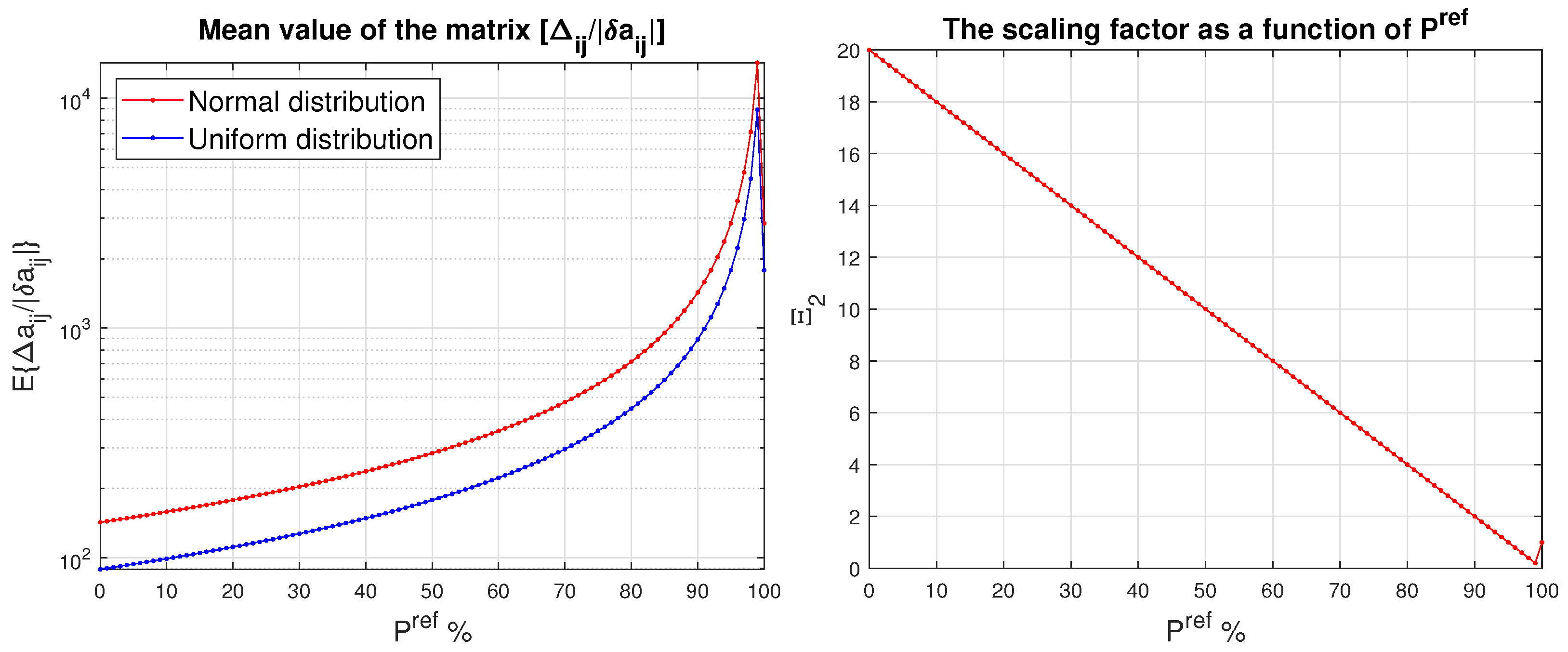
In Figure 9, we represent the mean value of the matrix [ Δ a i j / | δ a i j | ] and the scaling factor Ξ 2 as a function of P r e f . Since, in the given case we use δ A 2 instead of δ A F , the value of Ξ 2 = ( 1 P r e f ) m for a given probability P r e f is relatively small. For instance, if P r e f = 50 %, then we have that Ξ 2 = 10 and the mean value of [ Δ a i j / | δ a i j | ] is equal to 285.23 (Table 3).
In Figure 10, we compare the actual perturbations, δ σ i , of the singular values with the normwise bound (96) and the probabilistic bound (97) of the singular value perturbations for P r e f = 90 % , 80 % and 50 % . The probabilistic perturbation bound δ σ i e s t = δ A 2 / Ξ 2 is tighter than the normwise bound δ A 2 . Specifically, δ σ i e s t is 2 times smaller than δ A 2 for P r e f = 0.9 , 4 times for P r e f = 0.8 and 10 times for P r e f = 0.5 . The inequality | δ σ i | δ σ i e s t is satisfied for all singular values and probabilities due to the small values of Ξ 2 . Note that tighter probability estimates can be obtained if instead of δ A 2 we use δ A F and the scaling parameter Ξ = ( 1 P r e f ) m n .
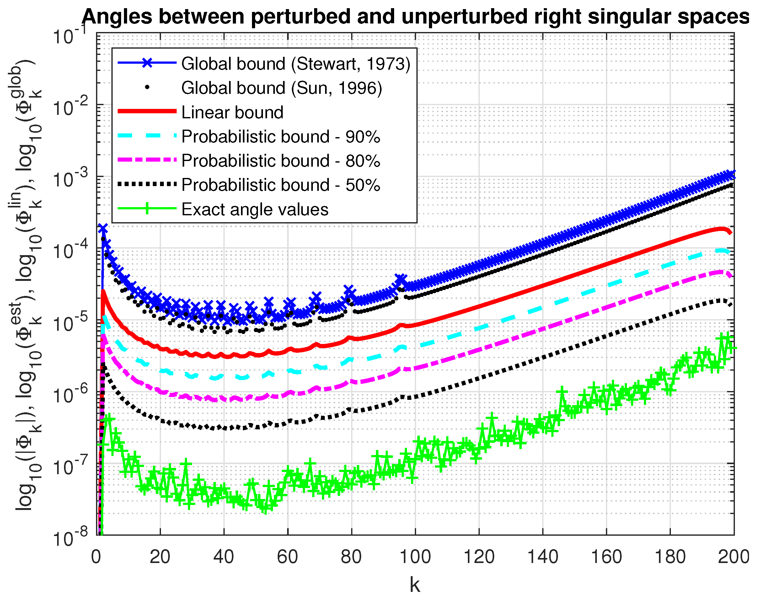
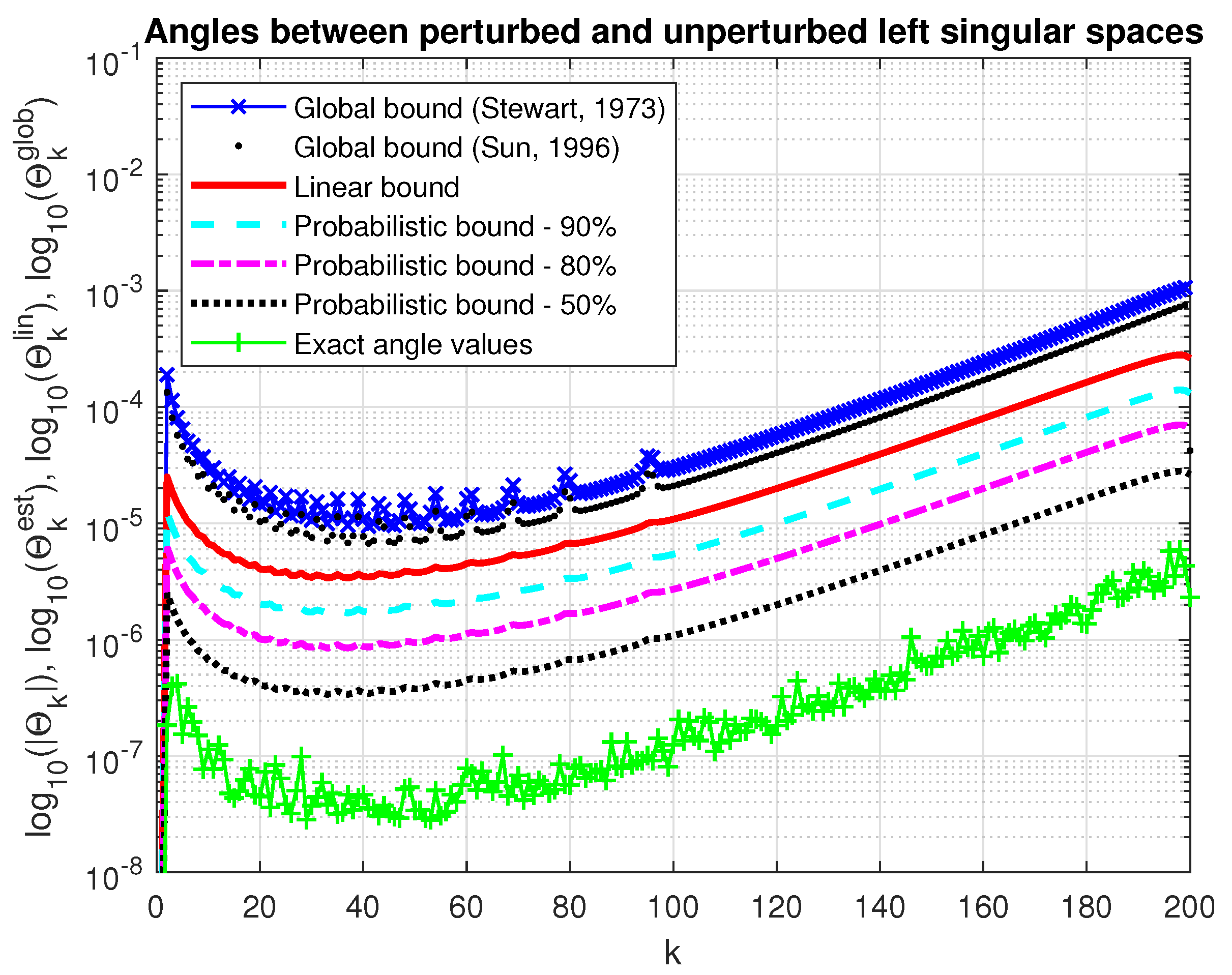
In Figure 11 and Figure 12, we show the actual values of the angles between the perturbed and unperturbed right and left singular subspaces, respectively, along with the corresponding linear bounds and probability bounds. For comparison, we give also the global bounds (69), (70) and (73), (74). As in the case of determining the deflation subspace global bounds, since the norms of parts of the perturbation matrix E are unknown, these norms are approximated by the 2-norms of the whole corresponding matrices. Clearly, the probabilistic bounds outperformall deterministic bounds. For instance, if P r e f = 0.5 , the probabilistic bounds are 10 times smaller than the deterministic asymptotic bound, as predicted by the analysis.
6. Conclusions

The splitting operator approach used in this paper allows us to derive unified asymptotic perturbation bounds of invariant, deflation and singular matrix subspaces that are comparable with the known perturbation bounds. These unified bounds make it possible to find easily probabilistic perturbation estimates of the subspaces that are considerably less conservative than the corresponding deterministic bounds, especially for high-order problems.
The proposed probability estimates have two disadvantages. First, they can be conservative due to the properties of the Markoff inequality so that the actual probability of the results obtained can be much better than those predicted by these estimates. Secondly, in the case of high-order problems, their computation requires much more memory than the known bounds due to the use of the Kronecker products.

Funding

This research received no external funding.

Notation

C ,the set of complex numbers;
j 0 = 1 ,the imaginary unit;
R ,the set of real numbers;
C n × m ,the space of n × m complex matrices;
R n × m ,the space of n × m real matrices;
A = [ a i j ] ,a matrix with entries a i j ;
a j ,the jth column of A;
a ¯ i j ,the complex conjugate of a i j ;
A i , 1 : n ,the ith row of an m × n matrix A;
A i 1 : i 2 , j 1 : j 2 ,the part of matrix A from row i 1
to i 2 and from column j 1 to j 2 ;
Low ( A ) ,the strictly lower triangular part of A;
Up ( A ) ,the strictly upper triangular part of A;
diag ( A ) ,the diagonal of A;
diag ( a 1 , a 2 , , a n ) ,the square matrix with diagonal elements equal to
a 1 , a 2 , , a n .
| A | ,the matrix of absolute values of the elements of A;
A T ,the transposed A;
A H ,the Hermitian conjugate of A;
A 1 ,the inverse of A;
0 m × n ,the zero m × n matrix;
I n ,the unit n × n matrix;
e j ,the jth column of I n ;
δ A ,the perturbation of A;
det ( A ) ,the determinant of A;
σ i ( A ) ,the ith singular value of A;
A 2 ,the spectral norm of A;
A F ,the Frobenius norm of A;
: = ,equal by definition;
⪯,relation of partial order. If a , b R n , then a b means
a i b i , i = 1 , 2 , , n ;
X = R ( X ) ,the subspace spanned by the columns of X;
U ,the unitary complement of U, U H U = 0 ;
A B ,the Kronecker product of A and B;
gap ( X , Y ) ,the gap between the subspaces X and Y ;
sep ( A , B ) ,the separation between A and B;
dif ( A , B ; C , D ) ,the difference between the spectra of A λ B and C λ D ;
vec ( A ) ,the vec mapping of A C n × m . If A is partitioned
columnwise as A = [ a 1 , a 2 , a m ] , then
vec ( A ) = [ a 1 T , a 2 T , , a m T ] T ;
P v e c ,the vec-permutation matrix. vec ( A T ) = P v e c vec ( A ) ;
P { y > y } ,the probability of the event { y > y } ;
E { ξ } ,the average value or mean of the random variable ξ ;
N { a i j b i j } ,the number of the entries of A that are
greater or equal to the corresponding entries of B.

Institutional Review Board Statement

Not applicable.

Informed Consent Statement

Not applicable.

Data Availability Statement

The datasets generated during the current study are available from the author upon reasonable request.

Acknowledgments

The author is grateful to the anonymous reviewers whose remarks and suggestions helped to improve the manuscript.

Conflicts of Interest

The author declares that the research was conducted in the absence of any commercial or financial relationships that could be construed as potential conflicts of interest.

References

  1. Stewart, G.W.; Sun, J.-G. Matrix Perturbation Theory; Academic Press: New York, NY, USA, 1990; ISBN 978-0126702309. [Google Scholar]
  2. Bhatia, R. Matrix factorizations and their perturbations. Linear Algebra Appl. 1994, 197–198, 245–276. [Google Scholar] [CrossRef]
  3. Li, R. Matrix perturbation theory. In Handbook of Linear Algebra, 2nd ed.; Hogben, L., Ed.; CRC Press: Boca Raton, FL, USA, 2014; ISBN 978-1-4665-0729-6. [Google Scholar]
  4. Adhikari, S.; Friswell, M.I. Random matrix eigenvalue problems in structural dynamics. Int. J. Numer. Methods Eng. 2006, 69, 562–591. [Google Scholar] [CrossRef]
  5. Benaych-Georges, F.; Enriquez, N.; Michail, A. Eigenvectors of a matrix under random perturbation. Random Matrices Theory Appl. 2021, 10, 2150023. [Google Scholar] [CrossRef]
  6. Benaych-Georges, F.; Nadakuditi, R.R. The eigenvalues and eigenvectors of finite, low rank perturbations of large random matrices. Adv. Math. 2011, 227, 494–521. [Google Scholar] [CrossRef]
  7. Cape, J.; Tang, M.; Priebe, C.E. Signal-plus-noise matrix models: Eigenvector deviations and fluctuations. Biometrika 2019, 106, 243–250. [Google Scholar] [CrossRef]
  8. Michaïl, A. Eigenvalues and Eigenvectors of Large Matrices under Random Perturbations. Ph.D. Thesis, Université Paris Decartes, Paris, France, 2018. Available online: https://theses.hal.science/tel-02468213 (accessed on 20 August 2024).
  9. O’Rourke, S.; Vu, V.; Wang, K. Eigenvectors of random matrices: A survey. J. Combin. Theory Ser. A 2016, 144, 361–442. [Google Scholar] [CrossRef]
  10. O’Rourke, S.; Vu, V.; Wang, K. Optimal subspace perturbation bounds under Gaussian noise. In Proceedings of the 2023 IEEE International Symposium on Information Theory (ISIT), Taipei, Taiwan, 25–30 June 2023; pp. 2601–2606. [Google Scholar] [CrossRef]
  11. Sun, J.-G. Perturbation expansions for invariant subspaces. Linear Algebra Appl. 1991, 153, 85–97. [Google Scholar] [CrossRef]
  12. Wilkinson, J. The Algebraic Eigenvalue Problem; Clarendon Press: Oxford, UK, 1965; ISBN 978-0-19-853418-1. [Google Scholar]
  13. Greenbaum, A.; Li, R.-C.; Overton, M.L. First-order perturbation theory for eigenvalues and eigenvectors. SIAM Rev. 2020, 62, 463–482. [Google Scholar] [CrossRef]
  14. Bai, Z.; Demmel, J.; Mckenney, A. On computing condition numbers for the nonsymmetric eigenproblem. ACM Trans. Math. Softw. 1993, 19, 202–223. [Google Scholar] [CrossRef]
  15. Stewart, G.W. On the sensitivity of the eigenvalue problem Ax=λBx. SIAM J. Numer. Anal. 1972, 9, 669–686. [Google Scholar] [CrossRef]
  16. Stewart, G.W. Error and perturbation bounds for subspaces associated with certain eigenvalue problems. SIAM Rev. 1973, 15, 727–764. [Google Scholar] [CrossRef]
  17. Sun, J.-G. Perturbation bounds for the generalized Schur decomposition. SIAM J. Matrix Anal. Appl. 1995, 16, 1328–1340. [Google Scholar] [CrossRef]
  18. Sun, J.-G. Perturbation analysis of singular subspaces and deflating subspaces. Numer. Math. 1996, 73, 235–263. [Google Scholar] [CrossRef]
  19. Kågström, B.; Poromaa, P. Computing eigenspaces with specified eigenvalues of a regular matrix pair (A,B) and condition estimation: Theory, algorithms and software. Numer. Algorithms 1996, 12, 369–407. [Google Scholar] [CrossRef]
  20. Benaych-Georges, F.; Nadakuditi, R.R. The singular values and vectors of low rank perturbations of large rectangular random matrices. J. Multivariate Anal. 2012, 111, 120–135. [Google Scholar] [CrossRef]
  21. Konstantinides, K.; Yao, K. Statistical analysis of effective singular values in matrix rank determination. IEEE Trans. Acoustic. Speech Signal Proc. 1988, 36, 757–763. [Google Scholar] [CrossRef]
  22. Liu, H.; Wang, R. An Exact sin Θ Formula for Matrix Perturbation Analysis and Its Applications; ArXiv e-prints in Statistics Theory [math.ST]; Cornell University Library: Ithaca, NY, USA, 2020; pp. 1–31. [Google Scholar] [CrossRef]
  23. O’Rourke, S.; Vu, V.; Wang, K. Random perturbation of low rank matrices: Improving classical bounds. Lin. Algebra Appl. 2018, 540, 26–59. [Google Scholar] [CrossRef]
  24. O’Rourke, S.; Vu, V.; Wang, K. Matrices with Gaussian noise: Optimal estimates for singular subspace perturbation. IEEE Trans. Inform. Theory 2024, 70, 1978–2002. [Google Scholar] [CrossRef]
  25. Wang, K. Analysis of Singular Subspaces under Random Perturbations; ArXiv e-Prints in Statistics Theory [math.ST]; Cornell University Library: Ithaca, NY, USA, 2024; pp. 1–68. [Google Scholar] [CrossRef]
  26. Wang, R. Singular vector perturbation under Gaussian noise. SIAM J. Matrix Anal. Appl. 2015, 36, 158–177. [Google Scholar] [CrossRef]
  27. Stewart, G.W. Stochastic perturbation theory. SIAM Rev. 1990, 32, 579–610. [Google Scholar] [CrossRef]
  28. Edelman, A.; Rao, N.R. Random matrix theory. Acta Numer. 2005, 14, 1–65. [Google Scholar] [CrossRef]
  29. Petkov, P. Probabilistic perturbation bounds of matrix decompositions. Numer Linear Alg. Appl. 2024. [Google Scholar] [CrossRef]
  30. Angelova, V.; Petkov, P. Componentwise perturbation analysis of the Singular Value Decomposition of a matrix. Appl. Sci. 2024, 14, 1417. [Google Scholar] [CrossRef]
  31. Konstantinov, M.; Petkov, P. Perturbation Methods in Matrix Analysis and Control; NOVA Science Publishers, Inc.: New York, NY, USA, 2020; Available online: https://novapublishers.com/shop/perturbation-methods-in-matrix-analysis-and-control (accessed on 20 August 2024).
  32. Petkov, P. Componentwise perturbation analysis of the Schur decomposition of a matrix. SIAM J. Matrix Anal. Appl. 2021, 42, 108–133. [Google Scholar] [CrossRef]
  33. Petkov, P. Componentwise perturbation analysis of the QR decomposition of a matrix. Mathematics 2022, 10, 4687. [Google Scholar] [CrossRef]
  34. Zhang, G.; Li, H.; Wei, Y. Componentwise perturbation analysis for the generalized Schur decomposition. Calcolo 2022, 59. [Google Scholar] [CrossRef]
  35. Stewart, G.W. Matrix Algorithms; Vol. II: Eigensystems; SIAM: Philadelphia, PA, USA, 2001; ISBN 0-89871-503-2. [Google Scholar]
  36. The MathWorks, Inc. MATLAB, Version 9.9.0.1538559 (R2020b); The MathWorks, Inc.: Natick, MA, USA, 2020; Available online: http://www.mathworks.com (accessed on 20 August 2024).
  37. Papoulis, A. Probability, Random Variables and Stochastic Processes, 3rd ed.; McGraw Hill, Inc.: New York, NY, USA, 1991; ISBN 0-07-048477-5. [Google Scholar]
  38. Horn, R.; Johnson, C. Matrix Analysis, 2nd ed.; Cambridge University Press: Cambridge, UK, 2013; ISBN 978-0-521-83940-2. [Google Scholar]
  39. Golub, G.H.; Van Loan, C.F. Matrix Computations, 4th ed.; The Johns Hopkins University Press: Baltimore, MD, USA, 2013; ISBN 978-1-4214-0794-4. [Google Scholar]
  40. Sun, J.-G. Stability and Accuracy. Perturbation Analysis of Algebraic Eigenproblems; Technical Report; Department of Computing Science, Umeå University: Umeå, Sweden, 1998; pp. 1–210. [Google Scholar]
  41. Davis, C.; Kahan, W. The rotation of eigenvectors by a perturbation. III. SIAM J. Numer. Anal. 1970, 7, 1–46. [Google Scholar] [CrossRef]
  42. Horn, R.; Johnson, C. Topics in Matrix Analysis; Cambridge University Press: Cambridge, UK, 1991; ISBN 0-521-30587-X. [Google Scholar]
  43. Bavely, C.A.; Stewart, G.W. An algorithm for computing reducing subspaces by block diagonalization. SIAM J. Numer. Anal. 1979, 16, 359–367. [Google Scholar] [CrossRef]
  44. Stewart, G.W. Matrix Algorithms; Vol. I: Basic Decompositions; SIAM: Philadelphia, PA, USA, 1998; ISBN 0-89871-414-1. [Google Scholar]
Figure 1. Mean value of [ Δ a i j / | δ a i j | ] as a function of P r e f (left) and the mean value of N { Δ a i j > | δ a i j | } / n 2 (right) as a function of P r e f for two random distributions of the entries of a 100 × 100 matrix.
Axioms 13 00597 g001
Figure 2. Eigenvalue perturbations and their linear and probabilistic bounds.
Axioms 13 00597 g002
Figure 3. Angles between the perturbed and unperturbed invariant subspaces and their bounds.
Axioms 13 00597 g003
Figure 4. Mean values of [ Δ a i j / | δ a i j | ] and [ Δ b i j / | δ b i j | ] for two random distributions as functions of P r e f .
Axioms 13 00597 g004
Figure 5. Mean values of N { Δ a i j > | δ a i j | } / n 2 and N { Δ b i j > | δ b i j | } / n 2 for two random distributions as functions of P r e f .
Axioms 13 00597 g005
Figure 6. Chordal metric perturbation bounds of the generalized eigenvalues.
Axioms 13 00597 g006
Figure 7. Angles between perturbed and unperturbed right deflating subspaces.
Axioms 13 00597 g007
Figure 8. Angles between perturbed and unperturbed left deflating subspaces.
Axioms 13 00597 g008
Figure 9. Mean value of the matrix [ Δ a i j / | δ a i j | ] (left) and the scaling factor (right) as a function of P r e f .
Axioms 13 00597 g009
Figure 10. Singular value perturbations and their bounds.
Axioms 13 00597 g010
Figure 11. Angles between the perturbed and unperturbed right singular subspaces.
Axioms 13 00597 g011
Figure 12. Angles between the perturbed and unperturbed left singular subspaces.
Axioms 13 00597 g012
Table 1. The mean value of the ratios [ Δ a i j / | δ a i j | ] and the relative number of entries for which N { Δ a i j > | δ a i j | } / n 2 , obtained for five values of P r e f , n = 100 .
P ref Ξ E { [ Δ a ij / | δ a ij | ] } N { Δ a ij > | δ a ij | } / n 2
% %
100.0 1.0000 × 10 0 6.3838 × 10 2 100.0000
90.0 1.0000 × 10 1 6.3838 × 10 1 100.0000
80.0 2.0000 × 10 1 3.1919 × 10 1 100.0000
60.0 4.0000 × 10 1 1.5959 × 10 1 98.8200
40.0 6.0000 × 10 1 1.0640 × 10 1 90.3400
Table 2. The mean value of the ratios [ Δ a i j / | δ a i j | ] and [ Δ b i j / | δ b i j | ] , obtained for three values of P r e f , n = 80 .
P ref Ξ E { [ Δ a ij / | δ a ij | ] } E { [ Δ b ij / | δ b ij | ] }
%
100.0 1.0000 × 10 0 5.5561 × 10 2 7.9274 × 10 2
90.0 8.0000 × 10 0 6.9451 × 10 1 9.9093 × 10 1
80.0 1.6000 × 10 1 3.4725 × 10 1 4.9546 × 10 1
Table 3. The mean value of the ratios [ Δ a i j / | δ a i j | ] and the relative number of entries for which N { Δ a i j > | δ a i j | } / n 2 , obtained for five values of P r e f , n = 100 .
P ref Ξ 2 E { [ Δ a ij / | δ a ij | ] } N { Δ a ij > | δ a ij | } / n 2
% %
100.0 1.0000 × 10 0 2.8523 × 10 3 100.0000
90.0 2.0000 × 10 0 1.4262 × 10 3 100.0000
80.0 4.0000 × 10 0 7.1309 × 10 2 100.0000
50.0 1.0000 × 10 1 2.8523 × 10 2 100.0000
20.0 1.6000 × 10 1 1.7827 × 10 1 100.0000
Disclaimer/Publisher’s Note: The statements, opinions and data contained in all publications are solely those of the individual author(s) and contributor(s) and not of MDPI and/or the editor(s). MDPI and/or the editor(s) disclaim responsibility for any injury to people or property resulting from any ideas, methods, instructions or products referred to in the content.