Combining Glimm’s Scheme and Operator Splitting for Simulating Constrained Flows in Porous Media

Abstract

This paper studies constrained Newtonian fluid flows through porous media, accounting for the drag effect on the fluid, modeled using a Mixture Theory perspective and a constitutive relation for the pressure—namely, a continuous and differentiable function of the saturation that ensures always preserving the problem hyperbolicity. The pressure equation also permits an ultra-small porous matrix supersaturation (that is controlled) and the transition from unsaturated to saturated flow (and vice versa). The mathematical model gives rise to a nonlinear, non-homogeneous hyperbolic system. Its numerical simulation combines Glimm’s method with an operator-splitting strategy to account for the Darcy and Forchheimer terms that cause the system’s non-homogeneity. Despite the Glimm method’s proven convergence, it is not adequate to approximate non-homogeneous hyperbolic systems unless combined with an operator-splitting technique. Although other approaches have already addressed this problem, the novelty is combining Glimm’s method with operator-splitting to account for linear and nonlinear drag effects. Glimm’s scheme marches in time using a formerly selected number of associated Riemann problems. The constitutive relation for the pressure—an increasing function of the saturation, with the first derivative also increasing, convex, and positive, enables us to obtain explicit expressions for the Riemann invariants. The results show the influence of the Darcy and Forchheimer drag terms on the flow.

1. Introduction

Transport phenomena in porous media present various applications, some of which with relevant environmental impacts, such as carbon dioxide sequestration (capturing and storing atmospheric carbon dioxide to reduce or avoid greenhouse gas emissions), penetration of chemical products contaminating the soil, or radioactive waste disposal. Among the significant petroleum applications are oil reservoir flow simulation, enhanced oil recovery (e.g., by waterflooding) and natural gas production, for instance. Another relevant application is groundwater flows (that may include contamination migration and may occur in aquifers—a geologic formation containing water that moves through it). Essentially, the study of groundwater flows is essential to the development and management of water resources.

Also, flows through porous media are applied to fuel cells (essentially hydrocarbon fuels and oxidant flow through porous media generating electricity and heat by electrochemical reactions), drying, filtration, geothermal energy management, drainage of agricultural lands, geothermal energy harvesting, solar energy collectors, and mass transfer through membranes, to cite some of the innumerous applications (see, for instance, [1,2,3,4,5,6,7]).

The volume averaging technique proposes conservation equations, hypotheses on the behavior of phases and interfaces, and constitutive assumptions at the microscopic scale, subsequently averaging the developed equations over a representative volume, referred to as REV, obtaining the equations on a macroscopic level. This methodology, initially proposed by Whitaker [8], is largely employed to describe flows through porous media. Some examples are Vafai and Tien [9], Vafai [10], Tien and Vafai [11], Alazmi and Vafai [12], Whitaker [13], and Goyeau et al. ([14].

The Mixture Theory, employed in the present work, always considers a macroscopic description of the superimposed continuous constituents of the mixture (each point in the mixture simultaneously occupied by all the mixtures’ constituents) with an apparent thermomechanical independence. The Mixture Theory adequately describes many relevant phenomena, such as the behavior of polymers (composite materials), flows through porous media or fluxes with liquid helium [15]. The conservation laws are proposed for all the constituents with additional supply terms to account for the interaction among the constituents (to deal with the constituents’ thermomechanical independence) and for the mixture as a whole (see, for instance, [16,17,18,19]). The mechanical model requires constitutive equations proposed by a systematic procedure, always satisfying the principle of objectivity and the second law of thermodynamics (e.g., [20,21]). Wang [22] employs a systematic approach using the principles of Continuum Mechanics (objectivity and the second law of thermodynamics) to propose a generalized Darcy’s law for a flow through a porous medium (in a macroscale), relating the pressure gradient, the fluid velocity and its gradient, accounting for the geometric and thermophysical properties’ effects.

Multi-scale models (e.g., [23,24,25,26]) employ conservation equations and make hypotheses on the behavior of phases and interfaces at the microscopic scale, subsequently averaging the developed equations over the REV, to obtain macroscale equations. A Mixture Theory approach is then employed on the macroscale to obtain the constitutive equations satisfying the second law of thermodynamics, giving rise to a complete mechanical model.

According to Hassanizadeh and Gray [24], the interaction stress in a Mixture Theory approach proposed by Williams [27] and Sampaio and Williams [28] is analogous to the interfacial stress used in their work [24].

There is no universal form of the second law of thermodynamics (or Clausius–Dühen inequality) used to impose restrictions on constitutive equations under a Mixture Theory context. Green and Naghdi [29] developed an entropy inequality to propose constitutive assumptions for a linear viscous fluid flowing through a linear elastic solid. Their results agree with those of Lindsay [30] regarding the flow of Newtonian fluid through an elastic solid. Considering incompressible mixtures, Costa Mattos et al. [21] proposed a systematic methodology to derive objective constitutive equations satisfying the second law by prescribing five thermodynamic potentials. The authors presented an example of an Ostwald de Waele fluid flowing through a rigid porous matrix. Francaviglia et al. [15] employed the Clausius–Dühen inequality to derive constitutive assumptions for a N component mixture with internal variables accounting for and neglecting viscosity.

Using a Mixture Theory viewpoint, Saldanha da Gama et al. [31] proposed a continuous and differentiable constitutive equation for the pressure as a function of the saturation with a continuous and increasing first derivative. The model allows for a tiny supersaturation—permitting the porous medium’s slightest deformation and maintaining the problem’s hyperbolical nature. The numerical simulation uses Glimm’s scheme, which marches in time using the solution of the associated Riemann problem. Saldanha da Gama et al. (2023) [31] presented a comprehensive review of previous works dealing with constrained hyperbolic flows through porous media and the transition of unsaturated–saturated flow. The present work may be considered an extension of [31] because the mechanical model is no longer reduced to a nonlinear non-homogeneous hyperbolic system. The non-homogeneous part of the operator is retained. Furthermore, concerning the approach used for Glimm’s method implementation, a variant of the classic Glimm’s method features four completely independent time-advance procedures. Each one of these procedures is endowed with its own random choice so that, at each time instant, the originated result corresponds to the average of these four evolutions employed.

The simulation combines Glimm’s scheme with an operator-splitting procedure, splitting away the time evolutionary part from the purely hyperbolic part. The article aims to describe the influence of the drag terms in the evolution of the saturation and velocity fields. This relationship used in this work for evaluating the drag term that contains a linear and a quadratic term (usually called Darcy and Forchheimer terms in the literature) with an important physical meaning has never been previously treated by employing a combination of Glimm’s scheme with a splitting procedure.

2. Mechanical Model

The mechanical model for the unsaturated flow through a porous medium considers a mixture of three chemically non-reacting continuous constituents with no phase change. There is a solid constituent representing the porous matrix, assumed to be very lightly deformable and at rest; a liquid constituent, which is an incompressible Newtonian fluid (denoted as the fluid constituent); and a minimal mass density gas constituent, included to account for the compressibility of the mixture. The solid and the gas constituents’ features do not require the conservation of mass and momentum to be satisfied for them. It must be fulfilled solely by the fluid constituent of the mixture, giving rise to the following system:

$$\begin{array}{l}{\displaystyle \frac{\partial {\rho }_F}{\partial t}}+\nabla \cdot ({\rho }_F{v}_F)=0\\ {\rho }_F\left[{\displaystyle \frac{\partial v_F}{\partial t}}+(\nabla v_F)v_F\right]=\nabla \cdot T_F+m_F+{\rho }_F{b}_F\end{array}.$$

(1)

In Equation (1), the equation in the first line refers to the mass balance, while the second one refers to the momentum balance. The index F represents the fluid constituent, with ${\rho }_F$ being its mass density and $v_F$ its velocity. Furthermore, $T_F$ is the partial stress tensor and $b_F$ is the body force per unit mass acting on it. The fluid constituent mass density represents the local ratio between its mass and the mixture’s whole volume. The fluid fraction $\varphi$ is defined as the ratio between the fluid constituent mass density (${\rho }_F$) and the actual fluid mass density (${\rho }_f$). This latter quantity is calculated using a Continuum Mechanics approach. The saturation $\psi$ is the ratio between the fluid fraction $\varphi$ and the porous medium porosity $\epsilon$ (also measured under a Continuum Mechanics approach). So, the following relations can be considered:

$$\varphi ={\displaystyle \frac{{\rho }_F}{{\rho }_f}}\hspace{1em}\mathrm{and}\hspace{1em}\psi ={\displaystyle \frac{\varphi }{\epsilon }}={\displaystyle \frac{{\rho }_F}{\epsilon {\rho }_f}}.$$

(2)

Furthermore, the partial stress tensor is assumed to be symmetrical in this work, automatically satisfying the angular momentum conservation for the fluid constituent.

The Mixture Theory requires additional source terms to account for the thermomechanical interaction among the mixtures’ constituents, and there is a momentum source acting on the fluid constituent represented by the term $m_F$ (with a dimension of force) because of the fluid constituent interaction with the remaining constituents of the mixture. The momentum source accounts for the drag force exerted by the solid constituent (representing the porous medium) and the negligible mass density gas constituent on the fluid constituent—referred to as the Darcy and Forchheimer terms [32,33] and for a term that attempts to model the capillary forces effect under a Mixture Theory viewpoint. Flows through unsaturated porous media present a strong dependency on the saturation, so the source term is assumed to depend also on the saturation gradient [27,34,35]:

$$m_F=-{\displaystyle \frac{{\mu }_f{\epsilon }^2}{K}}{\psi }^2{v}_F-{\displaystyle \frac{{\rho }_f{\epsilon }^2\overline{F}}{K^{1/2}}}{\psi }^2\left|v_F\right|v_F-{\displaystyle \frac{{\mu }_f{\epsilon }^{2}D}{K}}\hspace{0.17em}\nabla \psi .$$

(3)

where ${\mu }_f$ is the fluid viscosity, $\overline{F}$ is the Forchheimer number, and $K$ is the porous matrix specific permeability—all measured in a Continuum Mechanics context. The variable $D$ is a diffusion coefficient. In Equation (3), there are two drag terms; the first term exhibits a linear dependency on the fluid constituent velocity (the Darcy term), the second term presents a quadratic dependency on the fluid constituent velocity (the Forchheimer term). The third term in Equation (3), absent in saturated flows, mimics the capillary forces effect arising from the non-uniform fluid distribution in the porous matrix.

Williams [27], making an analogy with the Cauchy stress tensor, supposed the partial stress tensor $T_F$ to be proportional to the pressure and to the velocity gradient—namely to the rate of deformation tensor—acting on the fluid constituent. Allen [36] suggested the normal stresses dominance (over shear and interphase tractions) in the mixture, leading to a simplifying assumption for partial stress tensor acting on the fluid constituent $T_F$, i.e., it should be proportional to the pressure acting on it, as follows:

$$T_F=-\hspace{0.17em}\epsilon \hspace{0.17em}\psi \hspace{0.17em}\overline{p}\hspace{0.17em}I,$$

(4)

where $\overline{p}$ is a pressure and $I$ is the identity tensor.

Substituting the constitutive assumptions for the momentum source and the partial stress in the balance Equation (1), assuming that there is no influence of the body forces (essentially the gravity forces) on the flow, the following system results:

$$\begin{array}{l}{\displaystyle \frac{\partial {\rho }_F}{\partial t}}+\nabla \cdot ({\rho }_F{v}_F)=0\\ {\rho }_F\left[{\displaystyle \frac{\partial v_F}{\partial t}}+(\nabla v_F)v_F\right]=-\epsilon \hspace{0.17em}\nabla \left(\psi \overline{p}\right)-{\displaystyle \frac{{\mu }_f{\epsilon }^2}{K}}{\psi }^2{v}_F-{\displaystyle \frac{{\rho }_f{\epsilon }^2\overline{F}}{K^{1/2}}}{\psi }^2\left|v_F\right|v_F-{\displaystyle \frac{{\mu }_f{\epsilon }^{2}D}{K}}\nabla \psi \end{array}.$$

(5)

At this point, the variables are supposed to be functions solely of the time t and the coordinate on the flow direction x, with the fluid constituent velocity $v_F$ being indicated as u. In this case, the one-dimensional flow is expressed as follows:

$$\begin{array}{l}{\displaystyle \frac{\partial \psi }{\partial t}}+{\displaystyle \frac{\partial }{\partial x}}(\psi u)=0\\ {\rho }_f\left[\psi {\displaystyle \frac{\partial u}{\partial t}}+\left(\psi u\right){\displaystyle \frac{\partial u}{\partial x}}\right]=-{\displaystyle \frac{\partial }{\partial x}}\left(\psi \overline{p}\right)-{\displaystyle \frac{{\mu }_f{\epsilon }^2}{K}}{\psi }^{2}u-{\displaystyle \frac{{\rho }_f{\epsilon }^2\overline{F}}{K^{1/2}}}{\psi }^{2}u\left|u\right|-{\displaystyle \frac{{\mu }_f\epsilon D{\rho }_f^2}{K}}{\displaystyle \frac{\partial \psi }{\partial x}}\end{array}.$$

(6)

The system can be rewritten as:

$$\begin{array}{l}{\displaystyle \frac{\partial \psi }{\partial t}}+{\displaystyle \frac{\partial }{\partial x}}(\psi u)=0\\ {\displaystyle \frac{\partial }{\partial t}}(\psi u)+{\displaystyle \frac{\partial }{\partial x}}(\psi u^2)=-{\displaystyle \frac{1}{{\rho }_f}}{\displaystyle \frac{\partial }{\partial x}}\left(\psi \overline{p}\right)-{\displaystyle \frac{{\mu }_f{\epsilon }^2}{{\rho }_{f}K}}{\psi }^{2}u-{\displaystyle \frac{{\epsilon }^2\overline{F}}{K^{1/2}}}{\psi }^{2}u\left|u\right|-{\displaystyle \frac{{\mu }_f\epsilon D{\rho }_f}{K}}{\displaystyle \frac{\partial \psi }{\partial x}}\end{array}.$$

(7)

The pressure is conveniently expressed as follows:

$${\displaystyle \frac{\partial }{\partial x}}\left({\displaystyle \frac{\psi }{{\rho }_f}}\overline{p}\right)+{\displaystyle \frac{{\mu }_f\epsilon D{\rho }_f}{K}}{\displaystyle \frac{\partial \psi }{\partial x}}={\displaystyle \frac{\partial p}{\partial x}}.$$

(8)

The Darcy and the Forchheimer terms’ coefficients are conveniently expressed as follows:

$${\gamma }_1={\displaystyle \frac{{\mu }_f{\epsilon }^2}{\hspace{0.17em}{\rho }_{f}K}}\hspace{1em}\hspace{1em}\mathrm{and}\hspace{1em}\hspace{1em}{\gamma }_2={\displaystyle \frac{{\epsilon }^2\overline{F}}{K^{1/2}}}.$$

(9)

So, the mathematical model for the one-dimensional flow through porous media is expressed as follows:

$$\begin{array}{l}{\displaystyle \frac{\partial \psi }{\partial t}}+{\displaystyle \frac{\partial }{\partial x}}(\psi u)=0\\ {\displaystyle \frac{\partial }{\partial t}}(\psi u)+{\displaystyle \frac{\partial }{\partial x}}(\psi u^2+p)=-{\gamma }_1{\psi }^{2}u-{\gamma }_2{\psi }^2\left|u\right|u\end{array}.$$

(10)

The saturation $\psi$, defined in Equation (2), cannot exceed one. However, a supersaturation is allowed in this work, permitting a tiny deformation of the porous matrix (this deformation is so small that there is no need for the solid constituent to satisfy mass and momentum equations). In this context, the variable $\phi$ is the “enlarged” saturation, being given by the following:

$$\phi ={\displaystyle \frac{\varphi }{\epsilon +\delta }} \mathrm{with} \mathrm{the} \mathrm{original} \mathrm{saturation} \mathrm{satisfying}: \psi ={\displaystyle \frac{\varphi }{\epsilon }}<1+{\displaystyle \frac{\delta }{\epsilon }},\hspace{1em}\delta <<\epsilon .$$

(11)

It is important to note that this definition requires $\delta$ being a tiny positive constant. This minuscule supersaturation has already been considered in previous works, for instance, in [31,37].

The following constitutive relation is considered for the pressure [31]:

$$\begin{array}{l}p=\widehat{p}\left(\phi \right)=\phi +{\alpha }^2{\displaystyle \frac{\phi }{1-\phi }}-2\alpha \ln \left(1-\phi \right),\hspace{1em}\alpha \ge 0\\ \mathrm{with}\hspace{1em}\underset{p\to \infty }{\lim }\phi =1\end{array}.$$

(12)

The pressure $p$ was conveniently defined in Equation (8). It depends on the saturation and on a positive parameter $\alpha$. It should be noticed that Equation (12) supplies an upper bound for the saturation $\phi$, assuring a physically compatible and dependable simulation for the homogeneous portion of the hyperbolic operator of the one-dimensional flow described by Equation (10). The system hyperbolicity is ensured, regardless of the value of the fluid fraction, because the tiny, allowed supersaturation is controlled. An interesting and important feature of the constitutive relation for the pressure proposed for the pressure in Equation (12) is that the Riemann invariants can be expressed by closed-form expressions. This is very convenient for the simulation of the homogeneous portion via Glimm’s method. Also, the supersaturation has an a priori limit, even for enormous pressure values.

3. Numerical Procedure

The nonlinear non-homogeneous hyperbolic system, given by Equation (10), presented in the previous section, is simulated by combining Glimm’s method to simulate the homogeneous associated problem with an operator-splitting strategy to treat the non-homogeneous portion of the hyperbolic operator. The operator-splitting technique essentially treats a simultaneous protocol as a sequential one. It could be extended to more than one dimension; for instance, combined with a Godunov [38] scheme, it could simulate non-homogeneous two-dimensional hyperbolic systems. Although Glimm’s method has proven to capture discontinuities and shock waves with great accuracy, other well-known high-resolution schemes might also be employed. For a broad and updated review of these methods, the reader is referred to the work of Lochab and Kumar [39].

Combining an operator-splitting technique with Glimm’s scheme has been previously successfully used in numerous nonlinear hyperbolic problems with physical relevance. Sod [40] solved the gas dynamics flow equations with cylindrical symmetry, accounting for a converging cylindrical shock by combining Glimm’s method and operator splitting. Marchesin and Paes-Leme [41] simulated transient gas flows in pipelines using the gas dynamics equations to study shocks and spikes, accounting for Moody friction. They used Glimm’s scheme—a uniform sampling method—combined with an operator-splitting technique to account for Moody friction, which represents the non-homogeneous portion of the hyperbolic problem. Other examples include flows through unsaturated porous media [34,35,42], the response of nonlinear elastic rods [43], wave propagation in elasto-viscoplastic pipes subjected to damage [44], or transport of pollutants in the atmosphere [45,46,47].

Deng [48] presents different formulations of ROUND schemes (dissipative and low-dissipative) and observes that some low-dissipative ROUND schemes are extraordinarily accurate even when dealing with higher-order problems. Benchmark tests show ROUND’s superior performance on accuracy and resolution. Deng [48] also proposes a UND framework that unifies well-known second-order nonlinear schemes. His article highlights the current relevance of the theme. The much simpler and less expensive strategy used in this work can be supported by comparison with the exact solution of a Riemann problem, obtained by adjusting the initial condition and considering a limiting case in which the inhomogeneous terms tend to zero. It also allows for preserving the shock’s magnitude and position despite being a first-order scheme.

Considering the constitutive relation for the pressure presented in Equation (12), the following problem, subjected to known conditions at the time $t=t_n$, is to be approximated as follows:

$$\begin{array}{l}{\displaystyle \frac{\partial \phi }{\partial t}}+{\displaystyle \frac{\partial }{\partial x}}(\phi u)=0\\ {\displaystyle \frac{\partial }{\partial t}}(\phi u)+{\displaystyle \frac{\partial }{\partial x}}(\phi u^2+p)=-{\gamma }_1{\psi }^{2}u-{\gamma }_2{\psi }^2\left|u\right|u\\ \phi ={\left(\widehat{\phi }\right)}_n(x)\hspace{1em}\hspace{1em}\hspace{1em}\mathrm{at}\hspace{1em}\hspace{1em}t=t_n\\ \phi u={\left(\widehat{\phi }\widehat{u}\right)}_n(x)\hspace{1em}\hspace{1em}\mathrm{at}\hspace{1em}\hspace{1em}t=t_n,\end{array}.$$

(13)

with $\phi ={\left(\widehat{\phi }\right)}_n(x,t)$ and $\phi u={\left(\widehat{\phi }\widehat{u}\right)}_n(x,t)$.

It should be noted that this work is focused on something other than the convergence analysis of splitting procedures. A good example could be the convergence analysis of the Strang splitting algorithm for Vlasov-type equations, which is substantially used in electromagnetic field problems [49]. This work is focused on applying the operator-splitting technique combined with Glimm’s method. This procedure has been successfully used in the literature for various problems that are relevant to engineering, among which are a study of the damage induced by pressure transients in liquid-filled pipes at high temperatures [44], a study of the unsaturated flow through a rigid porous matrix accounting for a linear drag term [34] and a study of pollutant transport in the atmosphere when it can be used to account for the spherical geometry [46]. This work uses, for the first time, a combination of Glimm’s method and an operator-splitting technique to account for linear (Darcy) and nonlinear (Forchheimer) drag terms on a mixture theory model for an unsaturated flow through a porous matrix.

The first step is to use the decomposition below of the operator defined in Equation (13), allowing for its purely hyperbolic portion given by the homogeneous associated system, given by the following:

$$\begin{array}{l}{\displaystyle \frac{\partial \phi }{\partial t}}+{\displaystyle \frac{\partial }{\partial x}}(\phi u)=0\\ {\displaystyle \frac{\partial }{\partial t}}(\phi u)+{\displaystyle \frac{\partial }{\partial x}}(\phi u^2+p)=0\end{array}\hspace{0.17em}\mathrm{with}:$$

(14)

$$\begin{array}{l}\phi ={\left(\widehat{\phi }\right)}_n(x)\hspace{1em}\hspace{1em}\hspace{1em}\mathrm{at}\hspace{1em}\hspace{1em}t=t_n\\ \phi u={\left(\widehat{\phi }\widehat{u}\right)}_n(x)\hspace{1em}\hspace{1em}\mathrm{at}\hspace{1em}\hspace{1em}t=t_n\end{array},$$

(15)

to be separated from the time-evolutionary portion of the operator. The time evolutionary system is expressed as the following:

$$\begin{array}{l}{\displaystyle \frac{\partial \phi }{\partial t}}=0\hspace{1em}\Rightarrow \hspace{1em}\phi =\mathrm{constant}\\ {\displaystyle \frac{\partial }{\partial t}}(\phi u)=-{\gamma }_1{\phi }^{2}u-{\gamma }_2{\phi }^2\left|u\right|u\hspace{1em}\Rightarrow \hspace{1em}{\displaystyle \frac{\partial u}{\partial t}}=-{\gamma }_1\phi u-{\gamma }_2\phi \left|u\right|u\end{array}\hspace{0.17em}\mathrm{with}:$$

(16)

$$\begin{array}{l}\phi ={\left(\widehat{\phi }\right)}_{n+1}(x)\hspace{1em}\hspace{1em}\hspace{1em}\mathrm{at}\hspace{1em}\hspace{1em}t=t_n\\ \phi u={\left(\widehat{\phi }\widehat{u}\right)}_{n+1}(x)\hspace{1em}\hspace{1em}\mathrm{at}\hspace{1em}\hspace{1em}t=t_n\end{array}.$$

(17)

The numerical approximation from a given time step time $t_n$ to the successive time $t_n+\Delta t$ follows the subsequent development:

First, Glimm’s method is employed in Equations (14) and (15), allowing for us to obtain a preliminary approximation of the variables $\phi$ and $u$ (making an analogy with the predictor–corrector method, this would be the prediction step). A variant of the classic Glimm’s method is implemented in which four completely independent time-advance procedures (each one endowed with its own random choice) originate a result corresponding to the average of these four evolutions at each instant. These four sequences were employed independently, while the results were obtained from an arithmetic mean of the results of each sequence. This fact promoted a more accurate result, even for the first advance. It is remarkable that, in subsequent time instants, the evolution considers the results that originated it instead of considering the average of the results.

Subsequently, the same time step $\Delta t$ is employed in the “correction” step—namely the time evolutionary problem expressed by Equations (16) and (17), so that the solution’s approximation at the time $t_{n+1}$, given by $({\phi }_{n+1},\hspace{0.17em}{u}_{n+1})$ is reached, using as initial conditions the solution of Glimm’s method obtained in the previous “prediction” step. In this work, the approximation employs a first-order Euler approximation expressed as follows:

$$\begin{array}{l}{\displaystyle \frac{\partial u}{\partial t}}=-{\gamma }_1\phi u-{\gamma }_2\phi \left|u\right|u\\ u_{n+1}-u_n\approx \left[-{\gamma }_1\phi u_n-{\gamma }_2\phi \left|u_n\right|u_n\right]\Delta t\\ u_{n+1}=u_n+\left[-{\gamma }_1\phi u_n-{\gamma }_2\phi \left|u_n\right|u_n\right]\Delta t\end{array}.$$

(18)

The application of Glimm’s method with appropriate initial data for progressing Δt in time requires previous determination of the associated Riemann problem solution (or its approximation). The arbitrary initial condition—a function of the position is approximated by step functions, which are piecewise constant functions appropriately selected with equal-width steps because, for every two consecutive steps, a Riemann problem must be solved. The number of Riemann problems required for advancing from a time step $t_n$ to the successive time $t_{n+1}=t_n+\Delta t$ is previously chosen.

The combination of Glimm’s method with the splitting procedure allows for obtaining an approximation for the variables $\phi$ and $u$, repeating the described process until reaching a previously chosen simulation time. Note that, while Glimm’s method has a solid mathematical basis, the operator-splitting procedure has not been mathematically proven. However, it has been used by many different authors, as mentioned before.

Glimm’s method implementation also follows the same pattern described in detail by [31]. Some steps are reproduced to facilitate understanding of the methodology, since solving the problem described in the mechanical model requires Glimm’s method combination with an operator-splitting procedure. This latter is the main contribution of this work, allowing us to model problems that are physically more realistic.

Glimm’s method is a numerical technique that uses the solution of the associated Riemann problem, described in the Appendix A, to produce approximate solutions of the hyperbolic system subjected to arbitrary initial data. Glimm’s scheme suitably assembles a willingly selected number of Riemann problems to march sequentially from an instant n to a subsequent instant n + 1—it employs the Riemann problem’s solution for every two successive steps. The arbitrary initial condition—a function of the position must be approached by piecewise constant functions before using Glimm’s scheme and, consequently, finding the Riemann problem’s solution.

In other words, the initial condition for the homogeneous system presented in Equation (14) is such that:

$$\begin{array}{l}\phi (x,\hspace{0.17em}0)={\left(\phi \right)}_0(x)\\ \phi u(x,\hspace{0.17em}0)={\left(\phi u\right)}_0(x)\end{array}.$$

(19)

Equation (19) must be approximated by a piecewise constant function, and equal-width steps are adopted, so at a given time $t_i$:

$$\begin{array}{c}\phi ={\left(\widehat{\phi }\right)}_n(x)\approx {\left(\phi \right)}_{n_i}={\left(\widehat{\phi }\right)}_n\left(x_i+{\theta }_n\Delta x\right)\\ \phi u={\left(\widehat{\phi }\widehat{u}\right)}_n(x)\approx {\left(\phi u\right)}_{n_i}={\left(\widehat{\phi }\widehat{u}\right)}_n\left(x_i+{\theta }_n\Delta x\right)\end{array} \mathrm{for} x_i-{\displaystyle \frac{\Delta x}{2}}<x<x_i+{\displaystyle \frac{\Delta x}{2}}.$$

(20)

where ${\theta }_n\in \left(0,\hspace{0.17em}1\right)$ is a randomly chosen number and $\Delta x$ represents the width of the step. The generalized solution of the homogeneous problem (Equations (14) and (15)) at a time $t_{n+1}$ is given by the following:

$$\begin{array}{c}\overline{\phi }={\left(\tilde{\phi }\right)}_{n+1}(x)\approx {\left(\tilde{\phi }\right)}_{n_i}\hspace{0.17em}(x,\hspace{0.17em}{t}_{n+1})\\ \overline{\phi }\overline{u}={\left(\tilde{\phi }\tilde{u}\right)}_{n+1}(x)\approx {\left(\tilde{\phi }\tilde{u}\right)}_{n_i}\hspace{0.17em}(x,\hspace{0.17em}{t}_{n+1})\end{array}\hspace{1em}\mathrm{for}\hspace{0.17em}{x}_i<x<x_{i+1}.$$

(21)

Interactions among neighboring shocks of adjacent Riemann problems are avoided by choosing an interval $\Delta t$ so that the Courant–Friedrichs–Lewy (CFL) condition is always satisfied, ensuring the solution’s uniqueness, as follows:

$$\Delta t\le {\displaystyle \frac{\Delta x}{2{\left|\lambda \right|}_{\max }}}.$$

(22)

with ${\left|\lambda \right|}_{\max }$ representing the absolute value of the maximum shock speed considering all the Riemann problems at a specified time t. It should be emphasized that the time step used in the simulation is much smaller than the one required by the CFL condition to ensure the convergence of the operator-splitting technique. The chosen time step $\Delta t$ departed from the value given by the CFL condition given by Equation (22) and was reduced until the results were no longer affected by the time interval $\Delta t$. Note that this time step choice strategy has been previously employed (e.g., [34,35,45,47]).

4. Numerical Results

Since this work aims to describe the influence of the two components of the drag term on the evolution of saturation and velocity, namely the Darcy and Forchheimer term coefficients, the $\alpha$-parameter defined in the constitutive relation for the pressure, Equation (12), was not varied.

The results show the influence of two drag parameters, the Darcy and the Forchheimer terms coefficients, on the evolution of saturation and velocity. These two parameters that represent the linear and quadratic portion of the drag term on the momentum source, are given, respectively, by ${\gamma }_1$ and ${\gamma }_2$ and are defined in Equation (9). The $\alpha$-parameter is supposed very small ($\alpha =0.001$) throughout the article.

All the pictures in this section use a structure presenting the initial data for saturation and velocity in the first graph on the upper left side. The subsequent time instants march from left to right, following the first line of graphs and, subsequently, the second, third, and fourth (when present) ones, as indicated. The horizontal axis represents the coordinate on the flow direction x, varying from $-1.0$ to $+1.0$, while the vertical axis represents both the saturation $\phi$ and the velocity $u$.

The results are presented considering four distinct data sets. The first one (data set one) represents an initial value problem with initial data given by a step function for the saturation with $\phi$ $0.0\le x\le 1.0 : \phi =0.3$ and constant velocity defined by $\forall x : u=0.0$.

The second set (data set two) represents an initial value problem with initial data given by a distinct step function for the saturation with $-1.0\le x<-0.5 : \phi =0.5$ and $-0.5\le x\le 1.0 : \phi =0.3$, while, for velocity, the imposed initial condition is given by $-1.0\le x<-0.5 : u=0.0$, $-0.5\le x\le 0.0 : u=-1.0$, $0.0<x\le 0.5 : u=+1.0$, and $0.5<x\le 1.0 : u=0.0$.

Data sets three and four are initial value problems with boundary conditions. In both sets, the initial data are given by constant saturation ($\phi =0.2$) and velocity ($u=0$), but data set three considers a bounded domain with impermeable walls on the left and right sides. In contrast, in data set four, the bounded domain has a prescribed saturation on the left side and an impermeable wall on the right.

Figure 1, Figure 2 and Figure 3 depart from the same initial data, considering the initial data labeled data set one. In Figure 1, the Darcy and the Forchheimer terms are absent, while Figure 2 and Figure 3 present these terms. (in Figure 2 ${\gamma }_1=0.2$ and ${\gamma }_2=0.2$; while in Figure 3 ${\gamma }_1=2.0$ and and ${\gamma }_2=2.0$). The increase in the drag terms gives rise to a velocity decrease. When the drag effect is neglected (Figure 1, with ${\gamma }_1=0$ and ${\gamma }_2=0$), the higher velocities are obtained. Figure 2 and Figure 3 (the former with linear and quadratic drag term coefficients ten times smaller than the latter) are compared with Figure 1 (absence of drag). The drag presence provokes a “smoothing” effect on the saturation and velocity, which are almost constant after the eight-time interval.

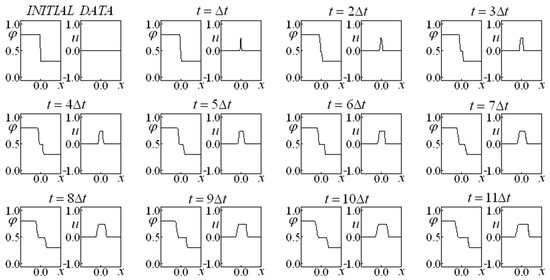
Figure 1. Saturation and Velocity Evolution for data set one, ${\gamma }_1=0$ and ${\gamma }_2=0$.

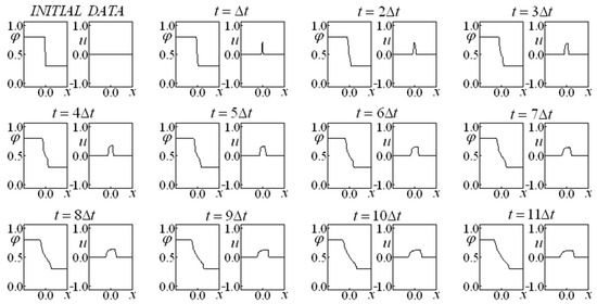
Figure 2. Saturation and Velocity Evolution for data set one, ${\gamma }_1=0.2$ and ${\gamma }_2=0.2$.

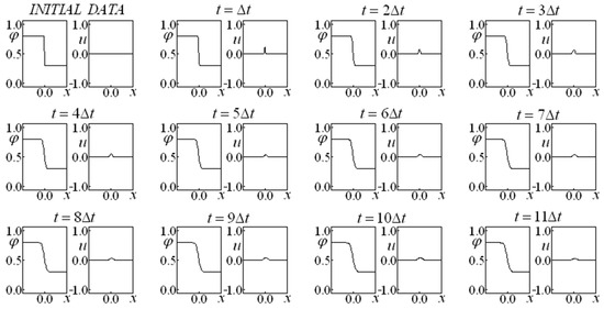
Figure 3. Saturation and Velocity Evolution for data set one, ${\gamma }_1=2.0$ and ${\gamma }_2=2.0$.

Figure 4, Figure 5, Figure 6, Figure 7, Figure 8 and Figure 9 present results obtained with initial data involving a nonzero velocity for several values of the parameters ${\gamma }_1$ and ${\gamma }_2$. Their initial data (data set two) imposes a step function for saturation and two distinct step functions for the velocity. Figure 4 represents the case in which there are no drag forces, while the other cases are affected by the drag presence. It may be noted that the higher the drag terms coefficients, the higher the “smoothing” effect on the saturation and velocity along the time.

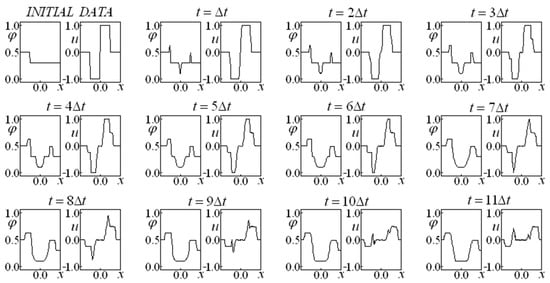
Figure 4. Saturation and Velocity Evolution for data set two, ${\gamma }_1=0$ and ${\gamma }_2=0$.

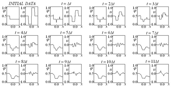
Figure 5. Saturation and Velocity Evolution for data set two, ${\gamma }_1=0.5$ and ${\gamma }_2=0.5$.

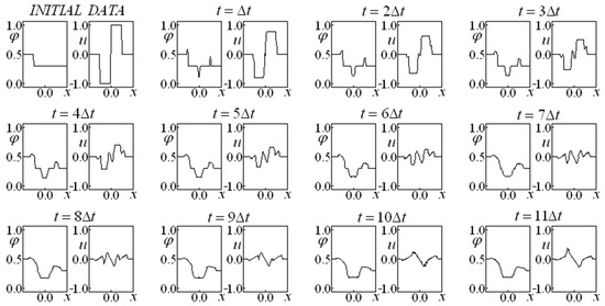
Figure 6. Saturation and Velocity Evolution for data set two, ${\gamma }_1=0.5$ and ${\gamma }_2=0.1$.

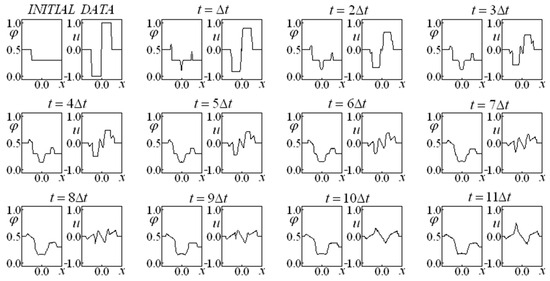
Figure 7. Saturation and Velocity Evolution for data set two, ${\gamma }_1=0.1$ and ${\gamma }_2=0.5$.

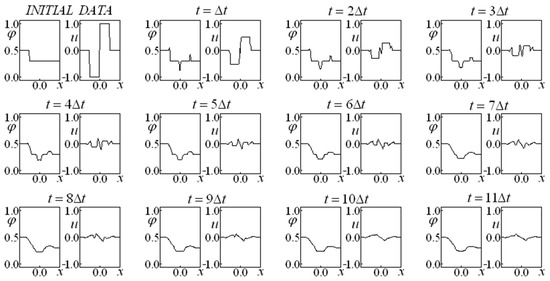
Figure 8. Saturation and Velocity Evolution for data set two, ${\gamma }_1=1.0$ and ${\gamma }_2=1.0$.

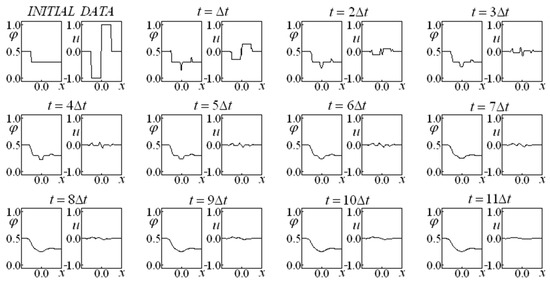
Figure 9. Saturation and Velocity Evolution for data set two, ${\gamma }_1=2.0$ and ${\gamma }_2=2.0$.

The comparison between Figure 6 (${\gamma }_1=0.5$ and ${\gamma }_2=0.1$) and Figure 7 (${\gamma }_1=0.1$ and ${\gamma }_2=0.5$) may lead to some interesting conclusions. The former (Figure 6) considers a higher coefficient for the linear drag term and a lower one for the nonlinear drag, while the latter (Figure 7) uses a smaller coefficient for the Darcy drag term and a larger one for the Forchheimer term. The “smoothness” effect is slightly higher in Figure 6 when the influence of the linear drag coefficient is stronger than the Forchherimer term coefficient.

Figure 10 and Figure 11 consider a bounded domain with impermeable walls on the left and right, departing from constant initial saturation and velocity. Comparing these two figures reveals the influence of the (linear and nonlinear) drag forces. In Figure 10, there are no drag forces (${\gamma }_1=0$ and ${\gamma }_2=0$), while, in Figure 11, the same drag coefficient is used for the linear and nonlinear terms (${\gamma }_1=1.0$ and ${\gamma }_2=1.0$).

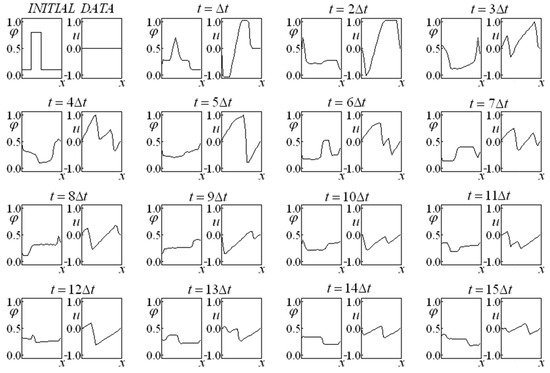
Figure 10. Saturation and Velocity Evolution for data set three, ${\gamma }_1=0$ and ${\gamma }_2=0$, with impermeable boundaries at both the left and right sides of the domain.

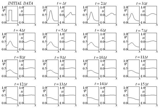
Figure 11. Saturation and Velocity Evolution for data set three, ${\gamma }_1=1.0$ and ${\gamma }_2=1.0$, with impermeable boundaries at both the left and right sides of the domain.

Figure 12, Figure 13, Figure 14 and Figure 15 present cases with a prescribed saturation on the left side and an impermeable wall on the right side, also departing from constant initial saturation and velocity, represented by data set four. The “smoothing” effect on the saturation and velocity provoked by the drag effect, observed on the unbounded problems (Figure 1, Figure 2, Figure 3, Figure 4, Figure 5, Figure 6, Figure 7, Figure 8 and Figure 9), is also observed when bounded problems (Figure 10, Figure 11, Figure 12, Figure 13, Figure 14 and Figure 15) are addressed, being more accentuated when the boundary condition is a prescribed saturation on one side and an impermeable wall at the other side.

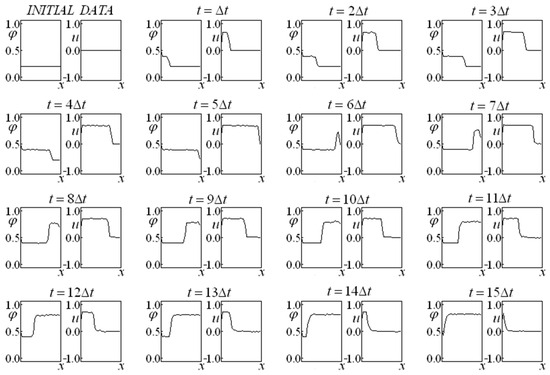
Figure 12. Saturation and Velocity Evolution for data set four, ${\gamma }_1=0$ and ${\gamma }_2=0$, with the prescribed saturation at the left side and the impermeable boundary at the right side.

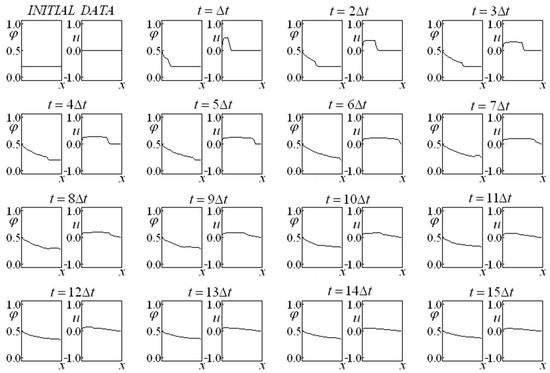
Figure 13. Saturation and Velocity Evolution for data set four, ${\gamma }_1=0.1$ and ${\gamma }_2=0.1$, with the prescribed saturation at the left side and impermeable boundary at the right side.

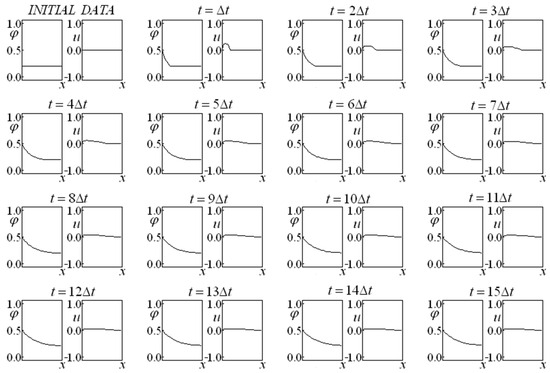
Figure 14. Saturation and Velocity Evolution for data set four, ${\gamma }_1=0.5$ and ${\gamma }_2=0.5$, with prescribed saturation at the left side and the impermeable boundary at the right side.

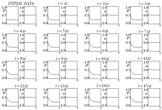
Figure 15. Saturation and Velocity Evolution for data set four, ${\gamma }_1=2.0$ and ${\gamma }_2=2.0$ with prescribed saturation at the left side and impermeable boundary at the right side.

5. Final Remarks

This article simulated a nonlinear, non-homogeneous hyperbolic system representing a mixture theory approach for constrained fluid flows through porous media, accounting for the so-called Darcy and Forchheimer terms (linear and nonlinear drag effects provoked by the porous matrix presence) on the momentum source term. The influence of these two components of the term representing drag is very relevant to real problems in engineering.

The numerical simulation combined a variant of Glimm’s method (that marches in time with a previously chosen number of associated Riemann problems) with an operator-splitting procedure. Glimm’s method variant considers four completely independent time-advance procedure evolutions (each with its own random choice) so that the average of the four evolutions gives the actual results. The operator-splitting technique is employed to deal with the system’s non-homogeneity. The convenient constitutive relation employed for treating the pressure allows for a tiny, controlled supersaturation of the porous matrix and enables explicit, closed-form expressions for the Riemann invariants. Note that this work combines Glimm’s scheme with an operator-splitting technique (a numerical procedure largely employed by several authors, with convenient modifications) to analyze the influence of the linear and nonlinear drag terms on the saturation and velocity fields of a porous matrix.

Applying this numerical technique to other problems involving nonlinear terms (like the drag term) in the non-homogeneous portion of the nonlinear hyperbolic system could be extended to previously studied problems. Examples include the distinct flows through porous media presented in [34], problems involving fluid flow and heat transfer [35] or pollutant transport problems in the atmosphere [45,46].

The simulated problems involved both unbounded domains (usual in initial value problems) and bounded domains with two different kinds of imposed boundary conditions.

This reliable tool can also adequately describe problems with transition saturated/unsaturated flow through porous media and vice versa, such as a development of Saldanha da Gama et al. (2023) [31] when the drag is maintained, resulting in a physically more realistic problem. Accurate numerical solutions would be provided by combining Glimm’s method with an operator-splitting procedure.

References

- Bear, J. Dynamics of Fluids in Porous Media; Courier Corporation: Dover, UK; New York, NY, USA, 1972. [Google Scholar]
- Bear, J. Hydraulics of Groundwater; Courier Corporation: Dover, UK; New York, NY, USA, 1979. [Google Scholar]
- Belghit, A.; Benyaich, M. Numerical Study of Heat Transfer and Contaminant Transport in an Unsaturated Porous Soil. J. Water Resour. Prot. 2014, 6, 1238–1247. [Google Scholar] [CrossRef][Green Version]
- Kaviany, M. Principles of Heat Transfer in Porous Media, Mechanical Engineering Series, 2nd ed.; Springer: Berlin/Heidelberg, Germany, 1995. [Google Scholar]
- Ma, L.; Ingham, D.B.; Pourkashanian, M.C. Application of fluid flows through. In Transport Phenomena in Porous Media III; Elsevier: Amsterdam, The Netherlands, 2005. [Google Scholar]
- Ingham, D.B.; Pop, I. Porous media in fuel cells. In Transport Phenomena in Porous Media III; Elsevier: Amsterdam, The Netherlands, 2005; pp. 418–440. [Google Scholar] [CrossRef]
- Scheidegger, A.E. The Physics of Flow through Porous Media, 3rd ed.; University of Toronto Press: Toronto, ON, USA, 1974. [Google Scholar]
- Whitaker, S. Advances in theory of fluid motion in porous media. Ind. Eng. Chem. 1969, 61, 14–28. [Google Scholar] [CrossRef]
- Vafai, K.; Tien, C.L. Boundary and Inertia Effects on Flow and Heat Transfer in Porous Media. Int. J. Heat Mass Transf. 1981, 24, 195–243. [Google Scholar] [CrossRef]
- Vafai, K. Convective Flow and Heat Transfer in Variable-Porosity Media. J. Fluid Mech. 1984, 147, 233–259. [Google Scholar] [CrossRef]
- Tien, C.L.; Vafai, K. Convective and radiative heat transfer in porous media. Adv. Appl. Mech. 1989, 27, 225–281. [Google Scholar] [CrossRef]
- Alazmi, B.; Vafai, K. Analysis of variants within the porous media transport models. J. Heat Transf. 2006, 122, 303–326. [Google Scholar] [CrossRef]
- Whitaker, S. The Forchheimer equation: A theoretical development. Transp. Porous Med. 1996, 25, 27–61. [Google Scholar] [CrossRef]
- Goyeau, B.; Benihaddadene, T.; Gobin, D.; Quintard, M. Averaged momentum equation for flow through a nonhomogeneous porous structure. Transp. Porous Med. 1997, 28, 19–50. [Google Scholar] [CrossRef]
- Francaviglia, M.; Palumbo, A.; Rogolino, P. Thermodynamics of mixtures as a problem with internal variables. Gen. Theory J. Non-Equilib. Thermodyn. 2006, 31, 419–429. [Google Scholar] [CrossRef]
- Atkin, R.J.; Craine, R.E. Continuum Theories of Mixtures. Basic Theory and Historical Development. Q. J. Mech. Appl. Math. 1976, 29, 209–244. [Google Scholar] [CrossRef]
- Bedford, A.; Drumheller, D.S. Theories of immiscible and structured mixtures. Int. J. Multiph. Flow 1983, 21, 863–960. [Google Scholar] [CrossRef]
- Bowen, R.M. Compressible porous media models by the use of the theory of mixtures. Int. J. Eng. Sci. 1982, 20, 697–735. [Google Scholar] [CrossRef]
- Rajagopal, K.R.; Tao, L. Mechanics of Mixtures, Vol. 35 of Advances in Mathematics for Applied Sciences; World Scientific: Singapore, 1995. [Google Scholar]
- Coleman, B.D.; Noll, W. The thermodynamics of elastic materials with heat conduction and viscosity. Arch. Ration. Mech. Anal. 1963, 13, 168–178. [Google Scholar] [CrossRef]
- Costa Mattos, H.S.; Martins-Costa, M.L.; Saldanha da Gama, R.M. On the modeling of momentum and energy transfer in incompressible mixtures. Int. J. Non-Linear Mech. 1995, 30, 419–431. [Google Scholar] [CrossRef]
- Wang, L. Flows through Porous Media: A Theoretical Development at Macroscale. Transp. Porous Med. 2000, 39, 1–24. [Google Scholar] [CrossRef]
- Gray, W.G.; Hassanizadeh, S.M. Unsaturated flow theory including interfacial phenomena. Water Resour. Res. 1991, 27, 1855–1863. [Google Scholar] [CrossRef]
- Hassanizadeh, S.M.; Gray, W.G. Mechanics and thermodynamics of multiphase flow in porous media including interphase boundaries, Adv. Water Res. 1990, 13, 169–186. [Google Scholar] [CrossRef]
- Murad, M.A.; Bennethum, L.S.; Cushman, J.H. A multiscale theory of swelling porous media I: Application to one-dimensional consolidation, Transp. Porous Media 1995, 19, 93–122. [Google Scholar] [CrossRef]
- Murad, M.A.; Cushman, J.H. Multiscale flow and deformation in hydrophilic swelling porous media. Int. J. Eng. Sci. 1996, 34, 313–338. [Google Scholar] [CrossRef]
- Williams, W.O. Constitutive equations for a flow of an incompressible viscous fluid through a porous medium. Q. J. Appl. Math. 1978, 36, 255–267. [Google Scholar] [CrossRef]
- Sampaio, R.; Williams, W.O. Thermodynamics of diffusing mixtures. J. Méc. 1979, 18, 19–45. [Google Scholar]
- Green, A.E.; Naghdi, P.M. The flow of fluid through an elastic solid. Acta Mech. 1970, 9, 329–340. [Google Scholar] [CrossRef]
- Lindsay, K.A. An application of a global entropy inequality to mixtures. Math. Proceed. Camb. Philos. Soc. 1973, 74, 185–197. [Google Scholar] [CrossRef]
- Saldanha da Gama, R.M.; Pedrosa Filho, J.J.; Saldanha da Gama, R.P.; da Silva, D.C.; Alexandrino, C.H.; Martins-Costa, M.L. Numerical Simulation of Constrained Flows through Porous Media Employing Glimm’s Scheme. Axioms 2023, 12, 1023. [Google Scholar] [CrossRef]
- Nield, D.A. The limitations of the Brinkmann-Forchheimer equations in modeling flow in a saturated porous medium and at the interface. Int. J. Heat Fluid Flow 1991, 12, 269–272. [Google Scholar] [CrossRef]
- Srinivasan, S.; Rajagopal, K.R. A thermodynamic basis for the derivation of the Darcy, Forchheimer and Brinkman models for flows through porous media and their generalizations. Int. J. Non-Linear Mech. 2014, 58, 162–166. [Google Scholar] [CrossRef]
- Martins-Costa, M.L.; Saldanha da Gama, R.M. Numerical simulation of one-dimensional flows through porous media with shock waves. Int. J. Numer. Methods Eng. 2001, 52, 1047–1067. [Google Scholar] [CrossRef]
- Saldanha da Gama, R.M.; Martins-Costa, M.L. Incompressible fluid flow and heat transfer through a nonsaturated porous medium. Comput. Mech. 1997, 20, 479–494. [Google Scholar] [CrossRef]
- Allen, M.B. Mechanics of multiphase fluid flows in variably saturated porous media. Int. J. Eng. Sci. 1986, 24, 339–351. [Google Scholar] [CrossRef]
- Martins-Costa, M.L.; Monte Alegre, D.; Freitas Rachid, F.B.; Jardim, L.G.C.M.; Saldanha da Gama, R.M. A hyperbolic mathematical modeling for describing the transition saturated/unsaturated in a rigid porous medium. Int. J. Non-Linear Mech. 2017, 95, 168–177. [Google Scholar] [CrossRef]
- Godunov, S.K. A Difference Scheme for Numerical Solution of Discontinuous Solution of Hydrodynamic Equations. Mat. Sb. 1959, 47, 271–307. (In Russian) [Google Scholar]
- Lochab, R.; Kumar, V. A comparative study of high-resolution methods for nonlinear hyperbolic problems. Z. Angew. Math. Mech. 2022, 102, e202100462. [Google Scholar] [CrossRef]
- Sod, G.A. A numerical study of a converging cylindrical shock. J. Fluid Mech. 1977, 83, 785–794. [Google Scholar] [CrossRef]
- Marchesin DPaes-Leme, P.J. Shocks in gas pipelines. SIAM J. Sci. Stat. Comput. 1983, 4, 105–116. [Google Scholar] [CrossRef]
- Saldanha da Gama, R.M.; Sampaio, R. A model for the flow of an incompressible Newtonian fluid through a nonsaturated infinite rigid porous medium. Comput. Appl. Math. 1987, 6, 195–205. [Google Scholar]
- Saldanha da Gama, R.M. An alternative procedure for simulating the dynamical response of non-linear elastic rods. Int. J. Numer. Methods Eng. 1990, 29, 123–139. [Google Scholar] [CrossRef]
- Freitas Rachid, F.B.; Saldanha da Gama, R.M.; Costa Mattos, H. Modelling the hydraulic transients in damageable elasto-viscoplastic piping systems. Appl. Math. Model. 1994, 18, 207–215. [Google Scholar] [CrossRef]
- Martins-Costa, M.L.; Saldanha da Gama, R.M. Glimm’s method simulation for the pollutant transport in an isothermal atmosphere. Comput. Mech. 2003, 32, 214–223. [Google Scholar] [CrossRef]
- Martins-Costa, M.L.; Saldanha da Gama, R.M. Simulation of pollutant motion and decay in polytropic atmospheres with spherical symmetry. Int. Commun. Heat Mass Transf. 2006, 33, 872–879. [Google Scholar] [CrossRef]
- Porto, E.M.; Martins-Costa, M.L.; Saldanha da Gama, R.M. An alternative procedure for simulating one-dimensional transport phenomena with shock waves in a gas. Int. J. Numer. Methods Biomed. Eng. 2011, 27, 157–172. [Google Scholar] [CrossRef]
- Deng, X. A unified framework for non-linear reconstruction schemes in a compact stencil. Part 1: Beyond second order. J. Comput. Phys. 2023, 481, 112052. [Google Scholar] [CrossRef]
- Einkemmer, L.; Ostermann, A. Convergence analysis of strang splitting for Vlasov-type equations. SIAM J. Numer. Anal. 2014, 52, 140–155. [Google Scholar] [CrossRef]
- Smoller, J. Shock-Waves and Reaction-Diffusion Equations; Cambridge University Press: New York, NY, USA, 1983. [Google Scholar]
Disclaimer/Publisher’s Note: The statements, opinions and data contained in all publications are solely those of the individual author(s) and contributor(s) and not of MDPI and/or the editor(s). MDPI and/or the editor(s) disclaim responsibility for any injury to people or property resulting from any ideas, methods, instructions or products referred to in the content. |
© 2024 by the authors. Licensee MDPI, Basel, Switzerland. This article is an open access article distributed under the terms and conditions of the Creative Commons Attribution (CC BY) license (https://creativecommons.org/licenses/by/4.0/).