Abstract
A nonlinear log-Birnbaum–Saunders regression model with additive errors is introduced. It is assumed that the error term follows a flexible sinh-normal distribution, and therefore it can be used to describe a variety of asymmetric, unimodal, and bimodal situations. This is a novelty since there are few papers dealing with nonlinear models with asymmetric errors and, even more, there are few able to fit a bimodal behavior. Influence diagnostics and martingale-type residuals are proposed to assess the effect of minor perturbations on the parameter estimates, check the fitted model, and detect possible outliers. A simulation study for the Michaelis–Menten model is carried out, covering a wide range of situations for the parameters. Two real applications are included, where the use of influence diagnostics and residual analysis is illustrated.
Keywords:
flexible log-Birnbaum–Saunders; flexible sinh-normal; influence diagnostics; Michaelis–Menten model; nonlinear regression MSC:
62E15; 62J02; 62J20
1. Introduction
Regression models are one of the most common statistical techniques used to explain the relationship between a response or output continuous variable Y and a given set of explanatory covariates or predictors , where p denotes the number of predictors. In the case where Y is a continuous random variable, linear models stand out as the most frequently used in practice. However, in certain situations, the relationship between the response variable and the set of predictors is nonlinear. In these cases, it is quite difficult to determine the nonlinear behavior of the response variable and the set of covariates. Nonlinear models usually arise from an underlying theory about the relationships between the variables under study. By definition, given a set of covariates and a function where are unknown parameters, f is linear in , , if and only if the first derivative of f with respect to does not depend on for ; otherwise, f is nonlinear. That is, in the nonlinear case, some of ’s parameters appear in f a nonlinear way.
One very general form of nonlinear regression model considers additive errors. Generally speaking, a nonlinear regression model with additive errors is defined as
where is a vector of unknown parameters, is a vector of known covariates, and is a nonlinear, injective, and continuous function, twice differentiable with respect to the elements of . The error terms are independent and identically distributed random variables. Usually it is assumed that with unknown . However, quite often, the assumption of normality of errors does not hold. Other alternative models should be considered. Among the most relevant ones, we can cite Cancho et al. [1], who proposed a nonlinear model where the error term follows Azzalini’s skew normal distribution introduced in [2], with skewness parameter , and scale parameter . Another nonlinear regression model with alpha power distributed errors was proposed in Martínez-Flórez et al. [3,4,5]. Details about the alpha power model can be seen in Durrans [6].
We highlight that all these precedents are unimodal. However, in practice, other situations are possible. As an introductory example of interest, consider, for instance, the distribution of RNA in patients with human immunodeficiency virus (HIV) undergoing highly active antiretroviral therapy (HAART). It can be seen in Li et al. [7] that the logarithm of RNA is an asymmetric bimodal distribution, which can be adjusted by a function of a given set of covariates, (for instance: level of certain biomarkers, sex, age, kind of diet, employment, etc.), and by using a nonlinear regression model with asymmetric and bimodal errors. In this context, we focus on nonlinear regression models based on the extension of the Birnbaum–Saunders (BS) distribution introduced in Martínez-Flórez et al. [8]. Our proposal may be superior for considering a mixture of distributions, since it involves fewer parameters. Influence diagnostics tools are also given. Following a traditional approach, different kinds of perturbations for the parameters in the model are introduced, which can be used to detect outliers and to assess the sensitivity of parameter estimates. Martingale-type residuals are proposed to check the fit provided by the model. All of these aim to illustrate the use of asymmetric nonlinear models to describe lifetime data.
The outline of this paper is as follows. In Section 2, the background of our proposal is established. In Section 3, the nonlinear flexible log-Birnbaum–Saunders regression model is introduced. Results from inferences based on the maximum likelihood method are given. The observed information Fisher matrix is obtained, along with its applications to this regression model. Due to the possible complexity of nonlinear models, a key point is to study the possible deficiencies in the fitted model. Therefore, Section 4 is devoted to influence diagnostics. First, the Cook generalized distance is considered. Later, local influence criteria are given to assess the effect of minor perturbations in the data and/or the proposed model on the statistical summaries. Different perturbation schemes are considered: case-weight as well as perturbation for the response variable, for explanatory variables, and for the scale parameter. Finally, martingale-type residuals are presented to detect deficiencies in the structural part of the model and detect possible outliers. A complete simulation study is given in Section 6. The two-parameter Michaelis–Menten model, widely used in kinetic chemistry, is considered. A variety of situations and error terms are covered. Two applications to real datasets can be seen in Section 7. There, a thoughtful discussion of different regression models is carried out. Moreover, the use of diagnostic criteria and residuals to improve the fitted nonlinear model is illustrated. Final conclusions are presented in Section 8. Technical details are provided in Appendix A.1, Appendix A.2 and Appendix A.3.
2. Materials and Methods
Recall that the BS distribution was introduced by Birnbaum and Saunders [9] in order to model the lifetime of certain structures under dynamic load and that a random variable (RV) T follows a BS distribution, if its probability density function (PDF) is
with , , and denoting the PDF of the distribution. In Equation (2), is a shape parameter, and is a scale parameter and the median of the distribution.
A number of regression models related to the BS distribution can be found in the literature. We first refer to the pioneering work carried out by Rieck and Nedelman [10], where the log-linear-Birnbaum–Saunders regression model was introduced. There, it was assumed that the output variable Y follows a sinh-normal (SHN) distribution, , whose PDF is
where is a shape parameter and is a location parameter. Given a random sample for , let . Rieck and Nedelman [10] proposed the linear regression model
where is a covariate vector, is a vector of unknown parameters, and the errors, , follow an SHN distribution, In this case, , and the errors are symmetric with respect to zero. Asymmetric extensions were proposed by Leiva et al. [11], who considered a skewed sinh-normal model and provided applications to pollution data in Santiago, Chile. Later, Lemonte et al. [12] proposed another asymmetric extension based on the skew-normal, and Martínez-Flórez et al. [3] introduced the asymmetric extension based on the alpha power model of Durrans [6].
Another kind of asymmetric generalization of the sinh-normal model was proposed in Martínez-Flórez et al. [8,13]. This is based on the flexible skew-normal distribution introduced in Gómez et al. [14], and it is known as the flexible sinh-normal (FSHN) distribution, , whose PDF is given by
with and denoting the cumulative distribution function (CDF) of the distribution. In Equation (5), is a shape parameter, is location, is scale, is related to the bimodality, and is skewness.
It can be seen in [8] that particular cases of interest in the FSHN model are:
- If , then the FSHN model reduces to the skewed sinh-normal distribution introduced by Leiva et al. [11].
- If then a symmetric model denoted as is obtained, which allows us to model symmetric bimodal data; see [8].
- If , then the FSHN model reduces to the sinh-normal distribution introduced by Rieck and Nedelman [10].
Furthermore, the following properties are proven in [8], which will be used subsequently.
Lemma 1.
Let . Then
- 1.
- with .
- 2.
- , .
- 3.
- , .
- 4.
- .
Remark 1.
Properties given in Lemma 1 allow us to obtain features of in terms of . For instance,
- 1.
- The p-th quantile of Y, , can be obtained from the p-th quantile, , of Z:
- 2.
- The moments of Y can be expressed in terms of the moments of the RV with . This fact will be explicitly introduced in the notation. So, we will write
Additional details can be seen in Martínez-Flórez et al. [8] and Gómez et al. [14].
The FSHN model was used in Martínez-Flórez et al. [8] to introduce the flexible Birnbaum–Saunders (FBS) linear regression model, which is based on the fact that, if , then
So, given a random sample from Equation (7), , covariates can be considered to explain the response variable in a natural way, that is,
This is called the flexible log-linear Birnbaum–Saunders regression model, whose details can be seen in [8].
In this paper, we consider a nonlinear extension of the model introduced in [8]. The interest of our proposal is based on the fact that there exist few papers dealing with nonlinear extensions of the log-BS regression model. We can cite the BS nonlinear regression model proposed by Lemonte and Cordeiro [15], the study on diagnostics and influence analysis techniques in nonlinear log-BS models with asymmetric models carried out by Lemonte [12], and the paper by Martínez-Flórez et al. [3] on the nonlinear log-BS exponentiated model.
3. Nonlinear Flexible Log-Birnbaum–Saunders
3.1. Regression Model
In this subsection, the flexible log-Birnbaum–Saunders nonlinear regression model is introduced. So, let us consider independent RVs with . Suppose now that the distribution of depends on a set of p explanatory variables, denoted by , in the following way:
- where is a p-dimensional vector of unknown parameters, and f is an injective and continuous nonlinear function, twice differentiable with respect to the elements of .
- The shape parameters do not involve ; that is, , and
Let Then, the nonlinear flexible log-Birnbaum–Saunders model is defined by
where it is assumed that the error terms, , are independent and identically distributed, Since , by applying results given in [8]
where
and is the variance of the RV with . The existence of and follow from , , where denotes the Napierian logarithm and the existence of moments of the skew-normal distribution [16]. Additional details can be seen in Appendix A.1.
Corollary 1.
Relevant nonlinear regression models that can be obtained as particular cases of the nonlinear flexible log-Birnbaum–Saunders are the following ones:
- 1.
- If , then the log-BS nonlinear regression model with asymmetric errors proposed by Lemonte and Cordeiro [15] is obtained.
- 2.
- If , then a nonlinear log-BS regression submodel with flexible sinh-normal errors is obtained. We highlight that this submodel may fit bimodal data for .
- 3.
- If , then the nonlinear extension of the Rieck and Nedelman regression model is obtained [10].
Proof.
Remark 2.
From now on, the following considerations must be taken into account:
- The general model with a scale parameter is considered, whose PDF was given in Equation (5). Also note that and .
- To emphasize the origin of our proposal, that is, the use of logarithm of a flexible Birnbaum–Saunders distribution as a regression model, the notation flexible log-Birnbaum–Saunders will be used instead of Both notations are equivalent.
3.2. Inference
In this subsection, the maximum likelihood method is applied to estimate the parameters in the model. To simplify the exposition of results, let us denote by
Proposition 1.
Let be a random sample of . Then, the log-likelihood function is
where , and denotes the function.
Proof.
Corollary 2.
Let be a random sample of . Then:
1. The score functions are
where denotes the sign function, and
2. Maximum likelihood estimators for the regression parameter and parameters are obtained as solutions for , which require numerical procedures.
Proof.
It is straightforward by applying standard calculus techniques. □
Observed Information Matrix
Let us consider the matrix
where is the Hessian matrix of the log-likelihood function . The elements of are denoted by . Their expressions are given in Appendix A.2.
Recall that the Fisher (or expected) information matrix, , is given by the expected values of the elements in . For large samples and under regularity conditions, the MLE of , , is asymptotically normal, and its asymptotic covariance matrix is the inverse of the Fisher information matrix, . Explicitly,
where denotes convergence in law or in distribution; see [17].
Let be the observed information matrix, which is obtained by replacing the unknown parameters in Equation (16) by their MLEs. Since, for large n, converges in probability to , in practice, Equation (17) is applied, taking instead of .
As for the existence of previous matrices, recall that the flexible skew-normal (FSN) and its properties are well-established. Our model is obtained by applying the transformation to an FSN variable. Therefore, taking into account that and functions are continuous and derivable, and given the good analytical properties of the FSN model, the existence of derivatives of log-likelihood in the nonlinear FLBS model follows. Moreover, for , the rows (or columns) of the information matrix are linearly independent. All these facts support that the MLEs’ regularity conditions are met in practice.
Moreover, for large n, and due to the convergence in probability of to , the inverse of submatrix in Equation (16), which corresponds to , , can be used to obtain the asymptotic variance of Specifically,
where is a matrix with , and denotes the i-th column of the matrix D evaluated at .
4. Influence Diagnostics
In this section, influence diagnostic tools are proposed. Specifically, Cook’s generalized distance is considered in Section 4.1. This is a case-deletion kind of influence diagnostic that can be used to detect influential observations on parameter estimates. Later, local influence measures are introduced in Section 4.2. Four perturbation schemes are proposed, which may be used to carry out a sensitivity study and detect influential cases affecting the obtained inferential results.
First, the notation is introduced. Following Cook [18], let be the log-likelihood corresponding to the model proposed in Equation (8), with being the vector of unknown parameters. Perturbations into the model can be introduced through a vector , which is restricted to some open subset . In practice, is a given perturbation scheme of the initial model.
Let us now consider to be the log-likelihood associated with the perturbed model for certain . It is assumed that there exists an such that for all ; that is, represents no perturbation into the model. It is also assumed that is twice continuously differentiable at (θ′ ), where θ′ and denote the transpose of and . Let us denote by and the MLEs of the unknown parameters under and , respectively.
The diagnostic curvature was introduced by Cook [18] as
where is an eigenvector of with , and is the matrix with elements . In practice, the elements of can be obtained from the relationship
evaluated at , with being the observed information matrix evaluated at and evaluated at and .
Based on Equation (18), the influence diagnostic analysis of maximum curvature, , can be carried out. So, the eigenvector associated with the largest eigenvalue of the matrix can be used to assess the local influence on the estimates of parameters in the log-BS nonlinear model. The effect of locally influential observations is determined by the perturbation of the data in the direction.
The previous tools can also be used to assess the local change in , due to the influence of , by using the likelihood displacement defined as which compares and with respect to the non-perturbed log-likelihood.
To conclude, it is worth mentioning that, in order to study influential observations, Poon and Poon [19] proposed the conformal normal curvature, , defined by
where is the trace of matrix Moreover, and are computationally equivalent. The conformal normal curvature in the direction is invariant under reparameterization and for any direction implying that is a normalized measure, which allows us to compare two curvatures.
4.1. Cook Generalized Distance
For the vector of parameters in the log-BS nonlinear model, , Cook’s generalized distance (GDC) measures the global effect on MLEs of when an observation is removed; details can be seen in [18]. If the number of regression coefficients in the fitted model is , then the global influential statistic for the log-FBS nonlinear regression model is given by
where is the estimated covariance matrix of , and is the MLE of when the -th observation is removed.
If we focus on the vector of regression coefficients , then we only need the subvector that corresponds to these coefficients, and Cook’s generalized distance reduces to
where is the submatrix of associated with vector
4.2. Local Influence Measurements
In this subsection, we deal with the effect of minor perturbations on the data, since they may cause a considerable effect on the estimates of parameters in the fitted model [20]. The local influence diagnostics are useful to check the model’s assumptions and assess the effects of minor perturbations in the dataset or in the proposed model on estimates of regression parameters, scale parameters, and other parameters. In this way, problems with the error distribution assumptions or the fitted regression model can be detected. The following perturbation schemes are addressed:
- Case-weight;
- Perturbation of the response variable;
- Perturbation of an explanatory variable;
- Perturbation of the scale parameter.
4.2.1. Case-Weight Perturbation
Let be the vector of case-weights for the log-FBS nonlinear regression model introduced in Equation (8). The relevant part of the log-likelihood for the perturbed model is
Then, for the -th observation and the j-th coefficient , it follows that
Therefore, the matrix is given by:
where is a matrix and
Moreover, is a matrix given by
where
4.2.2. Perturbation of the Response Variable
An additive perturbation scheme on the response variable is proposed as follows:
where is the standard deviation of the response variable, and . So, the relevant part of the perturbed log-likelihood is given by
where
In this case, the elements of the matrix are given by
where
4.2.3. Perturbation of an Explanatory Variable
Let us now consider the following additive perturbation for the explanatory variable :
where is the standard deviation of the variable, and Then, the relevant part of the perturbed log-likelihood is
where
and is
The elements of are
with and
Analogously, for parameters , and , we have that
where
4.2.4. Perturbation of a Scale Parameter
Now, we focus on the effect of a minor perturbation on the scale parameter , which may cause heteroscedasticity. In this subsection, the effect of this perturbation on the MLEs is studied. Let us assume that the error term in Equation (8) is distributed as , Then, the perturbed log-likelihood is
where
In this case, we have
and with
5. Residual Analysis
In this section, martingale-type residuals are considered to detect deficiencies in the fitted FBS nonlinear regression model with respect to the error distributional assumptions and to detect possible outliers. The study is based on the deviance component residual built on the martingale-type residuals proposed in Therneau et al. [21]. For the nonlinear log-FBS model, the martingale residuals can be obtained as
where is the CDF of the FSHN distribution, and .
Therneau et al. [21] proposed the deviance component residual as a transformation of the martingale-type residual. For non-censored data, they can be taken as
Here, can be used as martingale-type residuals since they are symmetrically distributed around zero.
On the other hand, Ortega et al. [22] proposed the consideration of the standardized residuals, . For the log-BS nonlinear model, they are given by
where is the i-th principal component for the generalized leverage matrix evaluated at ; details can be seen in Wei et al. [23].
The generalized leverage matrix is defined by
where is a Hessian matrix, and , with
and
In general, the distributions of martingale residuals and deviance component residuals are unknown. Based on the properties of deviance component residuals and the suggestions proposed in Atkinson [24], the residual analysis must be based on envelopes with normality plots. We will follow this recommendation in the practical applications carried out in Section 7.
6. Simulation
In order to study the performance of MLEs in the log-FBS nonlinear regression model, two simulation studies have been carried out. Both suggest the good performance of our proposal.
6.1. Simulation for the Two-Parameter Michaelis–Menten Model
Next, the two-parameter Michaelis–Menten model is introduced. This model is widely used in kinetic chemistry to describe the concentration of a substrate () in terms of the reaction rate (). In practice, it is applied to enzyme-catalyzed reactions of one substance and is used in a variety of situations, such as antigen–antibody binding, DNA–DNA hybridization, and protein–protein interactions.
The Michaelis–Menten model with log-FBS errors is given by
where the reaction rate , represents the maximum rate of reaction, is a kinetic constant, and
Properties of Equation (30) were studied by Cysneiros and Vanegas [25] by assuming that , , and the error term follows a Student’s distribution. In our simulation, we consider Equation (30) with these values of and , but the error term is FSHN distributed as
Without loss of generality, is fixed. For the shape parameters in the FSHN model, we take , and We highlight that these scenarios cover a variety of situations for the shapes of the FSHN distribution (unimodal and bimodal), as can be seen in [8].
As for the sample size, for every scenario, we consider For the explanatory variable , a random sample of a distribution was generated. In every setting, 2000 simulations were carried out by using the maxLik function of the R software and by applying the BFGS method. As statistical summaries, the standard deviation (sd) of MLEs, the absolute value of bias (), and the root of the mean squared error () are given in Table 1, Table 2, Table 3 and Table 4. In these tables, we can observe that, when the sample size increases, the standard deviations, biases, and decrease in all scenarios. It can also be determined that the bias and of and are negligible, which confirms the asymptotic unbiasedness of these estimators in the Michaelis–Menten model.

Table 1.
, sd, and for the MLEs in the nonlinear regression model.

Table 2.
, sd, and for the MLEs in the nonlinear regression model.

Table 3.
, sd, and for the MLEs of parameters in the nonlinear regression model.

Table 4.
, sd, and for the MLEs of parameters in the nonlinear regression model.
Also note that we obtained satisfactory results in our estimates for , suggesting the good performance of our model in bimodal settings.
For parameters, we highlight that the greater bias was obtained for and . However, if increases, then decreases. In all settings, the best results are obtained for negative values of , even for .
Since these simulations cover a variety of situations and shapes of the FSHN distribution, they suggest that the estimators of the parameters are consistent when the sample size increases.
As for the interest of our results in practice, we highlight the importance of the Michaelis–Menten model. Recall that, in kinetic chemistry, this model is applied in the classical case of an enzyme substrate mechanism in which the reaction timescale of the enzyme must be faster than the reaction timescale of the substrate.
6.2. Simulation for a Nonlinear Regression Model Proposed in [15]
A second simulation study is carried out for the nonlinear regression model with covariates, 4 regression coefficients, and sinh-normal errors discussed in Lemonte and Cordeiro [15]. The model is
Next, the MLE properties of parameters in this model are studied under the assumption of FSHN errors.
As statistical summaries, again we give: the standard error (sd) of estimates, , and .
The scenarios under consideration are: , and As for the parameters for the error term, we considered , and . The sample sizes in our simulations were The covariates were random variables generated as uniform . In every setting, the simulations were repeated 2000 times. The maxLik function of the R software and the BFGS method were applied.
Results are listed in Table 5 and Table 6. In general, we can see that the standard errors, the absolute bias, and the square root of the mean squared error decrease for all the parameters if the sample size increases.

Table 5.
, empirical sd, and for the MLEs of the parameters in the nonlinear regression model.

Table 6.
, empirical sd, and for the MLEs of the parameters in the nonlinear regression model.
We highlight that the estimates of parameters and , that is, for those involved in the regression model, behave well, which suggests their asymptotic unbiasedness and consistency.
7. Real Applications
In this section, two illustrations of the log-FBS nonlinear regression model are given. In Section 7.1, a discussion of linear and nonlinear regression models is carried out. The residual analysis techniques proposed in Section 5 are applied to check the model’s adequacy. On the other hand, in Section 7.2, the emphasis is put on the use of diagnostic influence techniques proposed in Section 4.
7.1. Illustration I
7.1.1. Classical Discussion of Models
Let us consider the Australian Institute of Sport (AIS) dataset available from the sn package of R [26]. It consists of measurements from high-performance athletes on various characteristics of the blood. We aim to explain the Hematocrit (Hc) variable in terms of Hemoglobin (Hg). A linear model with log-FBS errors and two nonlinear models with log-BS and log-FBS errors are considered for . First, it is established that a nonlinear model is better. Later, by using a likelihood ratio test (LRT), it is seen that a nonlinear model with log-FBS errors must be preferred. Its adequacy is checked by envelope plots for the martingale-type residuals.
The regression models under consideration are:
- Linear model for :where
- Nonlinear model for with log-BS errors:where
- Nonlinear model for with log-FBS errors:where
Table 7 provides the parameter estimates by using maximum likelihood, along with the estimated standard errors (in parentheses) and the p-values of tests for the coefficients. The proposed models are compared by using the Akaike information criterion (AIC) and corrected AIC (AICc) defined as
where is the number of parameters in the model. The better model is the one with the lowest AIC or AICc.

Table 7.
Parameter estimates (standard error) and p-values for nonlinear log-BS, linear log-FBS, and nonlinear log-FBS models, along with AIC and AICc values.
From AIC and AICc in Table 7, the nonlinear log-BS and nonlinear log-FBS models provide the better fit.
Since nonlinear log-BS and nonlinear log-FBS are nested models, they can be compared with a likelihood ratio test (LRT), where
and the test statistic is
By taking and using the estimates in Table 7, we obtain
which is greater than the critical point Therefore, the null hypothesis is rejected, and it can be stated than the nonlinear log-FBS model provides a better fit than the nonlinear log-BS one.
Moreover, Figure 1a,b give the envelopes for the martingale-type residuals for both nonlinear models. Again, these plots suggest that the nonlinear log-FBS model provides a better fit than the nonlinear log-BS one.
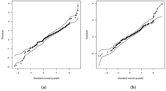
Figure 1.
Normal probability plots for with envelopes of Q-qplots for the scaled residuals for the fitted models: (a) nonlinear log-BS model and (b) nonlinear log-FBS model.
7.1.2. Discussion of Models Based on Validation Techniques
An evaluation of regression models previously proposed is next carried out by using validation techniques. Uses of cross-validation (CV) and generalized CV criteria to select models or optimal ridge parameters in partial linear regression models can be seen in [27,28], among others. In our case, we follow a validation approach.
We randomly split the 202 observations into two sets: a training set containing 101 of the data points, and a validation set with the remaining 101 observations. The regression model fitted to the training sample is later evaluated on the validation sample by using the mean squared error (MSE) as a measure of error. This process is repeated 100 times, that is, using 100 different random splits of the original sample into training and validation sets. In summary, the mean of the , , is given in Table 8.

Table 8.
MSE obtained for linear log-FBS, nonlinear log-BS, and nonlinear log-FBS models by using validation approach (50%, 50%), 100 times.
Since the nonlinear log-FBS model exhibits the smallest MSE in Table 8, this model would be preferred to describe our dataset.
As for goodness-of-fit tests to decide if the sample comes from a specific model, the Anderson–Darling test, implemented in the goftest R package, Version 1.2-3 is used [29]. The p-values of these tests are listed in Table 9. These summaries suggest that the nonlinear log-FBS model provides a good fit for this dataset.

Table 9.
Results for the Anderson–Darling goodness-of-fit test.
7.2. Illustration II: Model Discussion with Emphasis on the Use of Diagnostic Influence Techniques
The real dataset under consideration consists of 46 independent observations of a metal specimen subject to cyclic stress. This dataset has been previously studied by Rieck and Nedelman [10], Galea et al. [30] and Xie and Wei [31]. The variables involved in this study are: the response variable (), number of cycles to failure, and the explanatory covariable (), which corresponds to the work by cycle (mJ/m3). The aim is to check the number of cycles before a failure (crack) happens. Rieck and Nedelman [10] proposed to fit the linear regression model
where .
Note that Equation (31) is a linear model in the logarithm of the explanatory variable . This fact may render cumbersome the interpretation of parameters in the fitted model. An alternative is to keep the original explanatory variable and try to fit a nonlinear model. As for what nonlinear model to propose, the scatter plot of may be useful. In this case, an exponential model is suggested. So, we propose to fit the nonlinear regression model
where
Note that
with and
Remark 3.
A brief discussion to illustrate that, in this case, the nonlinear proposal is superior to the linear one is given in Appendix A.3.
The maximum likelihood estimates for the parameters in Equation (32) along with their standard errors (in parentheses) are given in Table 10.

Table 10.
Estimates of parameters in Equation (32).
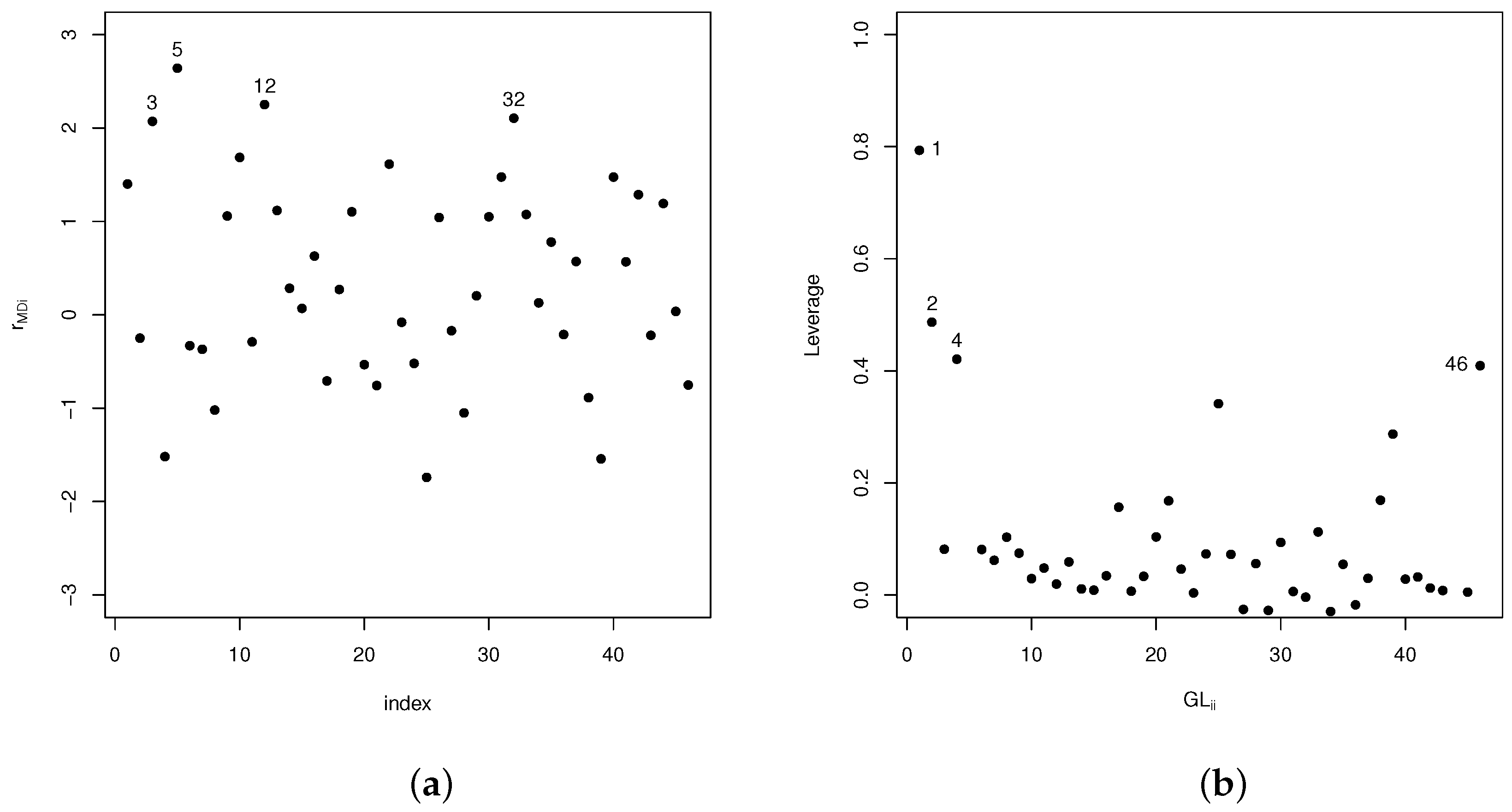
In Figure 2a,b, martingale-based residuals and the diagonal elements in matrix are plotted. These plots suggest that certain observations may be potentially influential. These are cases #1, #2, #3, #4, #5, #12, #32, and #46, among others.
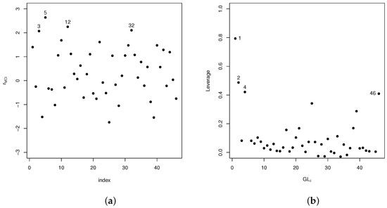
Figure 2.
(a) Plots of deviance component residuals . (b) Elements in the diagonal of the generalized Leverage matrix .
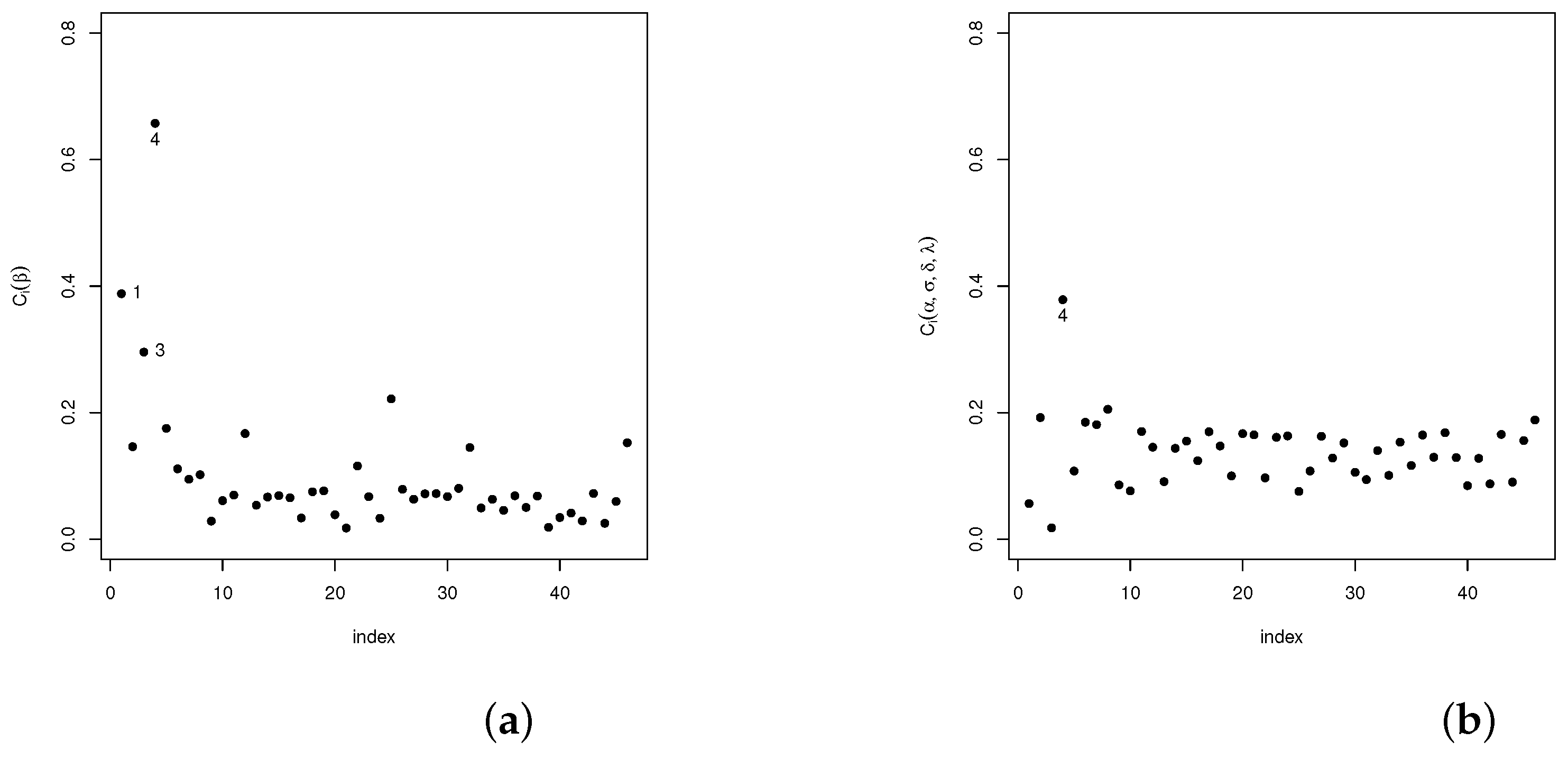
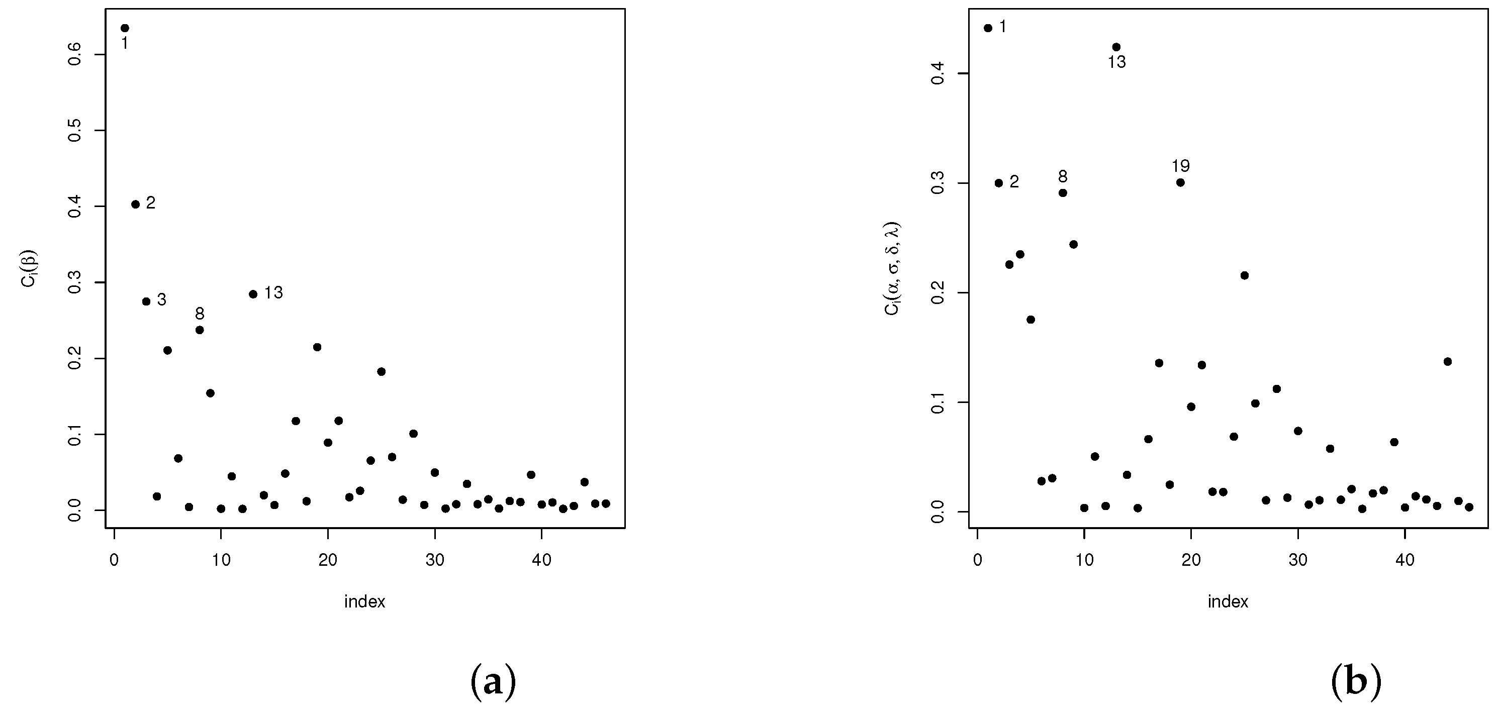
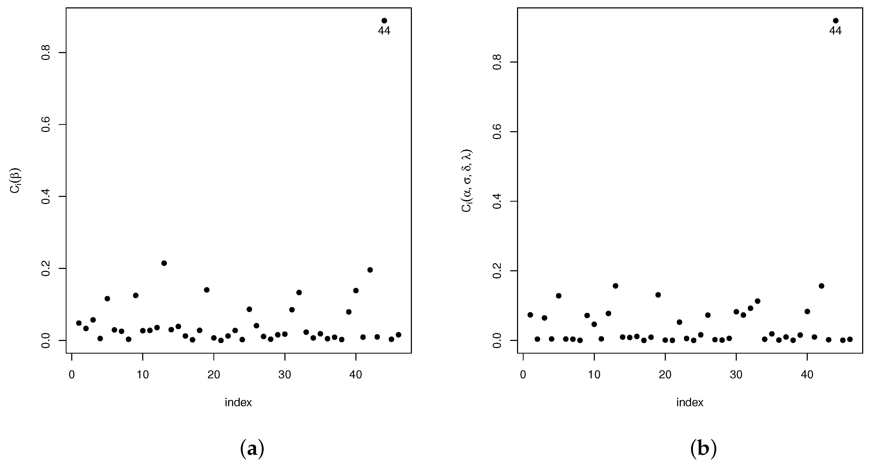
Analogously, diagnostic analyses have been carried out for the vector of parameter and the remaining parameters in the model . The statistic introduced in Section 4.1 is used in the following settings: case-weights, perturbation of the response variable, perturbed covariables, and perturbed scale parameters. Our results show that, in the case-weights setting, cases #1, #3, and #4 are detected as potentially influential, whereas for the perturbed response variable and the perturbed scale parameter setting, only case #44 was detected as potentially influential. As for the perturbed covariable setting, cases #1, #2, #3, #8, #13, and #19 are detected. The plots given in Figure 3a,b, Figure 4a,b, Figure 5a,b and Figure 6a,b show the results of these analyses.
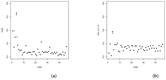
Figure 3.
Plots for the index in the case-weights scheme: (a) for and (b) for .
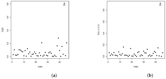
Figure 4.
Plots for the index in the perturbation of the response variable scheme: (a) for and (b) for .
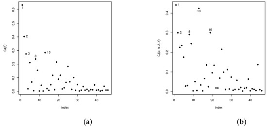
Figure 5.
Plots for the index in the perturbed covariate scheme: (a) for and (b) for .
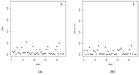
Figure 6.
Plots for the index for the perturbation of the scale parameter scheme: (a) for and (b) for .
Next, the influence of previously mentioned cases is studied thorough the relative change statistic, defined as
where denotes the maximum likelihood estimate for the parameter , including all observations, and denotes the estimate of the same parameter, deleting the influential observations.
The approximation for the standard error (SE) of proposed in Santana et al. [32] will be used:
where denotes the SE for the maximum likelihood estimate for the parameter , including all observations, and denotes the SE for the estimate of the same parameter, deleting the influential observations.
Table 11 provides the , their in parentheses, and the p-values associated with test versus for

Table 11.
Relative change, (, and p-values for model parameters.
From the results in Table 11, we may conclude that, individually, cases #2, #44, and #46 affect the estimates of the parameters and in the nonlinear regression model, as well as the scale (), shape (), and skewness () parameters. It can also be seen that cases #2 and #46 have influence on the ML-estimator of
Moreover, the joint influence of cases , and is analyzed. It can be seen that, jointly, these observations have influence on the estimates of the model parameters. As for the hypothesis tests for the parameters in the nonlinear regression model, none of the observations (#2, #44, and #46) affect their significance.
Therefore, cases #2, #44, and #46 were eliminated. The new fitted model is
whose error terms are distributed as
The plots in Figure 7a,b show the envelope plot for the martingale-type residuals and the dispersion plot for the final fitted model given in Equation (33). Both plots suggest that this is a good choice for describing this dataset.
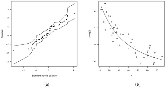
Figure 7.
(a) Normal probability plots for with envelopes of Q-qplots for the scaled residuals from the fitted model and (b) dispersion diagram for nonlinear model FSHN with errors.
8. Conclusions
In this paper, a nonlinear log-Birnbaum–Saunders regression model with additive errors is introduced. It is assumed that the errors follow the flexible sinh-normal distribution introduced in [8]. As an advantage, we highlight that this model can be used to describe a continuous response variable with asymmetric, unimodal, or bimodal behavior by using a nonlinear function of covariates. Its theoretical properties are studied, along with results from the maximum likelihood estimation of the parameters. Influence diagnostics are introduced in order to provide tools to detect influential observations and deficiencies in the fitted model. Statistics based on Cook’s generalized distance and local influence diagnostics are considered. Several perturbation schemes are proposed. Specifically, these are: case-weight, perturbations of the response variable, perturbations of an explanatory variable, and perturbations of the scale parameter. Martingale-type residual analysis is presented to detect deficiencies in the fitted model. Simulation studies are included, where the Michaelis–Menten model of interest in kinetic chemistry is considered. The simulations cover a variety of situations as for the range of parameters under consideration. In particular, we highlight that negative and positive values for the parameter that controls the unimodality or bimodality in our model are considered. Our results suggest that the estimators of the parameters are consistent and show the good performance in both unimodal and bimodal settings. To conclude, applications to real datasets are given in order to illustrate how to use our methodology.
We highlight that, in the first application, a discussion of linear and nonlinear regression models is carried out, first from a classical point of view. Several information criteria and the likelihood ratio test are applied. Martingale-type residual analysis techniques are applied to check the model’s adequacy. Second, this discussion is also carried out by using cross-validation techniques. In both cases, our proposal is superior to the other regression models under consideration. On the other hand, in the second real application, the emphasis is on the use of diagnostic influence techniques to detect influential observations.
As important novelties and advantages of our model, we highlight the nonlinearity of our proposal and the kind of distribution used for the errors, since it is assumed that they follow a flexible sinh-normal distribution. Therefore, it is useful for modeling unimodal and bimodal settings. Also, recall that it can be applied to nonnegative data and that it is of interest in reliability and medicine. Moreover, our approach is more general and reduces to other nonlinear regression models previously introduced in the literature, such as the log-BS nonlinear regression model with asymmetric errors introduced in [15].
As future research, we will consider the extension of these models to a censored continuous response variable . This kind of study is relevant, for instance, in medicine, where, quite often, we have data that can only be recorded above or below a certain threshold and that depend on the sensitivity of a laboratory test.
Author Contributions
Conceptualization, G.M.-F., I.B.-C. and H.W.G.; formal analysis, G.M.-F., I.B.-C. and H.W.G.; investigation, G.M.-F., I.B.-C. and H.W.G.; methodology, G.M.-F., I.B.-C. and H.W.G.; software, G.M.-F.; supervision, H.W.G.; validation, G.M.-F. and I.B.-C.; visualization, H.W.G. All authors have read and agreed to the published version of the manuscript.
Funding
The research of H.W. Gómez was supported by Grant SEMILLERO UA-2024 (Chile). The research of I. Barranco-Chamorro was supported by IOAP of the University of Seville, Spain. The research of G. Martínez-Flórez was supported by the Vice-rectorate for Research of the Universidad de Córdoba, Colombia, project grant FCB-06-22.
Data Availability Statement
Details about data availability have been given in Section 7. The numerical code is available upon request.
Conflicts of Interest
The authors declare no conflicts of interest.
Abbreviations
The following abbreviations for distributions are used in this manuscript:
| BS | Birnbaum–Saunders |
| SHN | sinh-normal |
| FSHN | flexible sinh-normal |
| FBS | flexible Birnbaum–Saunders |
| FLBS | flexible log-Birnbaum–Saunders |
Appendix A
Appendix A.1
Lemma A1.
Let Then,
where
and denotes the variance of the RV with .
Proof.
Since , it can be seen in [8] that , with . Recall that the PDF of is
Therefore,
Taking into account the relationship , , and the fact that, if , then (see Love [33]), then we have that
can be expressed in terms of incomplete moments of the skew-normal distribution. The existence of moments of the skew-normal distribution can be seen in Haas [16]; therefore, also exists.
Note that we can proceed similarly for or with , since the moments of the skew-normal distribution exist; see Haas [16]. Therefore, the moments of with also exist, in particular, . □
Appendix A.2
Next, the elements of the observed information matrix are given.
Corollary A1.
Let be a random sample of . Then, the elements of the observed information matrix are:
where
Proof.
It is straightforward by applying standard calculus techniques. □
Appendix A.3
In this appendix, it is shown that the nonlinear model proposed in Section 7.2 is superior to a linear model. So, for the dataset studied in Section 7.2, let us consider the linear model with sinh-normal errors or log-BS
with . Summaries for this model and the nonlinear one proposed in Equation (32) are given in Table A1. From AIC and AICc in Table A1, it can be concluded that the nonlinear flexible log-BS provides a better fit to this dataset than the linear log-BS model.

Table A1.
Parameter estimates (standard errors).
Table A1.
Parameter estimates (standard errors).
| Estimates | Log-BS | Flexible Log-BS |
|---|---|---|
| 0.5202 (0.0543) | 2.3061 (1.3846) | |
| p-value | (0.0000) | (0.0479) |
| 7.9849 (0.1546) | 10.1725 (1.4170) | |
| p-value | (0.0000) | (0.0000) |
| −0.0406 (0.0033) | −5.8413 (1.0844) | |
| p-value | (0.0000) | (0.0000) |
| −17.9475 (8.5355) | ||
| p-value | (0.0354) | |
| 0.9499 (0.3100) | ||
| p-value | (0.0021) | |
| 1.2984 (0.6121) | ||
| p-value | (0.0339) | |
| −5.6195 (2.6171) | ||
| p-value | (0.0317) | |
| AIC | 75.5638 | 53.6077 |
| AICc | 76.5394 | 56.5550 |
References
- Cancho, V.G.; Lachos, V.H.; Ortega, E.M.M. A nonlinear regression model with skew-normal errors. Stat. Papers 2010, 51, 547–558. [Google Scholar] [CrossRef]
- Azzalini, A. A class of distributions which includes the normal ones. Scand. J. Stat. 1985, 12, 171–178. [Google Scholar]
- Martínez-Flórez, G.; Bolfarine, H.; Gómez, H.W. The Log-Linear Birnbaum–Saunders Power Model. Methodol. Comput. Appl. Probab. 2017, 19, 913–933. [Google Scholar] [CrossRef]
- Bolfarine, H.; Martínez–Flórez, G.; Salinas, H.S. Bimodal symmetric-asymmetric families. Commun. Stat. Theory Methods 2018, 47, 259–276. [Google Scholar] [CrossRef]
- Martínez-Flórez, G.; Bolfarine, H.; Gómez, H.W. An alpha-power extension for the Birnbaum–Saunders distribution. Statistics 2014, 48, 896–912. [Google Scholar] [CrossRef]
- Durrans, S.R. Distributions of fractional order statistics in hydrology. Water Resour. Res. 1992, 28, 1649–1655. [Google Scholar] [CrossRef]
- Li, X.; Chu, H.; Gallant, J.E.; Hoover, D.R.; Mack, W.J.; Chmiel, J.S.; Muñoz, A. Bimodal virologic response to antiretroviral therapy for HIV infection: An application using a mixture model with left censoring. J. Epidemiol. Commun. Health 2006, 60, 811–818. [Google Scholar] [CrossRef]
- Martínez-Flórez, G.; Barranco-Chamorro, I.; Gómez, H.W. Flexible Log-Linear Birnbaum–Saunders Model. Mathematics 2021, 9, 1188. [Google Scholar] [CrossRef]
- Birnbaum, Z.W.; Saunders, S.C. A New Family of Life Distributions. J. Appl. Probab. 1969, 6, 319–327. [Google Scholar] [CrossRef]
- Rieck, J.R.; Nedelman, J.R. A log-linear model for the Birnbaum–Saunders distribution. Technometrics 1991, 33, 51–60. [Google Scholar]
- Leiva, V.; Vilca-Labra, F.; Balakrishnan, N.; Sanhueza, A. A skewed sinh-normal distribution and its properties and application to air pollution. Commun. Stat. Theory Methods 2010, 39, 426–443. [Google Scholar] [CrossRef]
- Lemonte, A.J. A log-Birnbaum–Saunders regression model with asymmetric errors. J. Stat. Comput. Simul. 2012, 82, 1775–1787. [Google Scholar] [CrossRef]
- Martínez-Flórez, G.; Barranco-Chamorro, I.; Bolfarine, H.; Gómez, H.W. Flexible Birnbaum–Saunders Distribution. Symmetry 2019, 11, 1305. [Google Scholar] [CrossRef]
- Gómez, H.W.; Elal-Olivero, D.; Salinas, H.S.; Bolfarine, H. Bimodal extension based on the skew-normal distribution with application to pollen data. Environmetrics 2011, 22, 50–62. [Google Scholar] [CrossRef]
- Lemonte, A.J.; Cordeiro, G. Birnbaum–Saunders nonlinear regression models. Comput. Stat. Data Anal. 2009, 53, 4441–4452. [Google Scholar] [CrossRef]
- Haas, M. A Note on the Moments of the Skew-Normal Distribution. Econ. Bull. 2012, 32, 3306–3312. [Google Scholar]
- Lehman, L.E. Elements of Large-Sample Theory; Springer: New York, NY, USA, 1999. [Google Scholar]
- Cook, R.D. Assessment of Local Influence. J. R. Stat. Society Ser. B (Methodol.) 1986, 48, 133–169. [Google Scholar] [CrossRef]
- Poon, W.Y.; Poon, Y.S. Conformal normal curvature and assessment of local influence. J. R. Statist. Soc. B 1999, 61, 51–61. [Google Scholar] [CrossRef]
- Barros, M.; Galea, M.; Gonzalez, M.; Leiva, V. Influence diagnostics in the tobit censored response’ model. Stat. Methods Appl. 2010, 19, 379–397. [Google Scholar] [CrossRef]
- Therneau, T.; Grambsch, P.; Fleming, T. Martingale based residuals for survival models. Biometrika 1990, 77, 147–160. [Google Scholar] [CrossRef]
- Ortega, E.M.; Bolfarine, H.; Paula, G.A. Influence diagnostics in generalized log-gamma regression models. Comput. Stat. Data Anal. 2003, 42, 165–186. [Google Scholar] [CrossRef]
- Wei, B.C.; Hu, Y.Q.; Fung, W.K. Generalized leverage and its applications. Scand. J. Stat. 1998, 25, 25–37. [Google Scholar] [CrossRef]
- Atkinson, A.C. Two graphical displays for outlying and influential observations in regression. Biometrika 1981, 68, 13–20. [Google Scholar] [CrossRef]
- Cysneiros, F.J.A.; Vanegas, L.H. Residuals and their statistical properties in symmetrical nonlinear models. Stat. Probab. Lett. 2008, 78, 3269–3273. [Google Scholar] [CrossRef]
- Azzalini, A. The R Package ’sn’: The Skew-Normal and Related Distributions such as the Skew-t and the SUN (Version 2.1.1). Available online: https://cran.r-project.org/package=sn (accessed on 15 August 2024).
- Wasserman, L. All of Nonparametric Statistics; Springer Science+Business Media Inc.: New York, NY, USA, 2006. [Google Scholar]
- Amini, M.; Roozbeh, M. Optimal partial ridge estimation in restricted semiparametric regression models. J. Multivar. Anal. 2015, 136, 26–40. [Google Scholar] [CrossRef]
- Baddeley, B. Goftest: Classical Goodness-of-Fit Tests for Univariate Distributions. R Package Version 1.2-3. Available online: https://cran.r-project.org/web/packages/goftest (accessed on 5 June 2024).
- Galea, M.; Leiva-Sánchez, V.; Paula, G.A. Influence diagnostics in log-Birnbaum–Saunders regression models. J. Appl. Stat. 2004, 31, 1049–1064. [Google Scholar] [CrossRef]
- Xie, F.C.; Wei, B.C. Diagnostics analysis for log-Birnbaum–Saunders regression models. Comput. Statist. Data Anal. 2007, 51, 4692–4706. [Google Scholar] [CrossRef]
- Santana, L.; Vilca, F.; Leiva, V. Influence analysis in skew-Birnbaum–Saunders regression models and applications. J. Appl. Stat. 2011, 38, 1633–1649. [Google Scholar] [CrossRef]
- Love, E.R. Some Logarithm Inequalities. Math. Gaz. 1980, 64, 55–57. [Google Scholar] [CrossRef]
Disclaimer/Publisher’s Note: The statements, opinions and data contained in all publications are solely those of the individual author(s) and contributor(s) and not of MDPI and/or the editor(s). MDPI and/or the editor(s) disclaim responsibility for any injury to people or property resulting from any ideas, methods, instructions or products referred to in the content. |
© 2024 by the authors. Licensee MDPI, Basel, Switzerland. This article is an open access article distributed under the terms and conditions of the Creative Commons Attribution (CC BY) license (https://creativecommons.org/licenses/by/4.0/).


