An Efficient Anti-Noise Zeroing Neural Network for Time-Varying Matrix Inverse

Abstract

The Time-Varying Matrix Inversion (TVMI) problem is integral to various fields in science and engineering. Countless studies have highlighted the effectiveness of Zeroing Neural Networks (ZNNs) as a dependable approach for addressing this challenge. To effectively solve the TVMI problem, this paper introduces a novel Efficient Anti-Noise Zeroing Neural Network (EANZNN). This model employs segmented time-varying parameters and double integral terms, where the segmented time-varying parameters can adaptively adjust over time, offering faster convergence speeds compared to fixed parameters. The double integral term enables the model to effectively handle the interference of constant noise, linear noise, and other noises. Using the Lyapunov approach, we theoretically analyze and show the convergence and robustness of the proposed EANZNN model. Experimental findings showcase that in scenarios involving linear, constant noise and noise-free environments, the EANZNN model exhibits superior performance compared to traditional models like the Double Integral-Enhanced ZNN (DIEZNN) and the Parameter-Changing ZNN (PCZNN). It demonstrates faster convergence and better resistance to interference, affirming its efficacy in addressing TVMI problems.

1. Introduction

The problem of time-varying matrix inversion (TVMI) often arises in various scientific and engineering fields. For instance, in the field of image processing, TVMI is used in real-time image restoration and denoising algorithms to enhance image quality and accuracy [1]. In the field of robotics, TVMI is applied to motion control and path planning in dynamic environments to ensure that robots can adjust and execute complex tasks in real time [2]. In the field of signal processing, TVMI is used for real-time filtering and signal recovery, especially when dealing with time-varying signals and systems [3,4]. In robotic kinematics, TVMI is used to solve kinematic inverse problems to achieve precise control and operation of robotic arms [5], among other applications. Currently, the methods to solve matrix inversion problems primarily fall into the following two categories: numerical algorithms and neural network algorithms. Numerical algorithms are essentially serial processes and are primarily suitable for small-scale and constant matrices. For example, the authors of [6] employed the iteration method to solve matrix inversion; however, the iterative process is highly complex and time-consuming [7]. Unlike traditional numerical methods, neural network methods have advantages such as parallel processing capabilities and distributed storage [8], which have been widely studied. For example, Gradient-based Recurrent Neural Networks (GNNs) [9] are used for static matrix inversion, significantly improving computational efficiency. However, many studies have reported that GNNs struggle to capture changes in variable coefficient matrices and are primarily designed for time-invariant problems [10], rendering them unsuitable for dynamic situations [11].

To effectively address the problem of the TVMI, Zhang and colleagues introduced a novel ZNN model [12] that leverages the time derivative of the error function to achieve exponential decay of the error over an indefinitely long period, effectively solving time-varying problems [13]. Furthermore, numerous scholars have continuously innovated and improved upon the ZNN framework, proposing derivatives of the ZNN models for time-varying problems. For example, the author of [14] proposed a Finite-Time ZNN (FTZNN) model that achieves finite-time convergence for the TVMI problem through a new design formula, significantly improving convergence performance compared to existing recurrent neural networks (such as GNNs) and the original ZNN model. The authors of [15] introduced the Classical Complex-Valued Noise-Tolerant ZNN (CVNTZNN) model, which was developed to address the Dynamic Complex Matrix Inversion (DCMI) problem; the authors explored the performance of the CVNTZNN model in various noise environments. Another study [16] proposed a Fixed-Time Convergent and Noise-Tolerant ZNN (FTCNTZNN) model, demonstrating superior fixed-time convergence and robustness in both noiseless and noisy environments when solving the TVMI problem.

As research has progressed, scholars have faced key issues such as convergence, robustness, and stability when using ZNN models to solve TVMI problems [17,18,19]. In terms of improving convergence, studies have shown that the design parameters of a ZNN have a significant impact on convergence speed [20]. Traditional ZNN models typically use fixed convergence parameters, and while these models can achieve effective convergence [21], the fixed parameters often require multiple additional experiments to adjust and find approximately optimal parameters. This process is inefficient and difficult to implement in practical applications. In practical applications, convergence parameters generally correspond to the inverse of inductance or capacitance in circuits [22], meaning that convergence parameters are time-varying in hardware systems. Moreover, because larger design parameter values result in better convergence, recent studies have explored various variable-parameter ZNN models to solve the TVMI problem more quickly. For example, the authors of [23] proposed a novel Exponential-enhanced-type Varying-Parameter ZNN (EVPZNN) model that significantly improves convergence speed compared to traditional Fixed-Parameter ZNN (FPZNN) [10]. In [24], P.S. Stanimirovic and others introduced a new segmented varying-parameter approach to establish a Complex Varying-Parameter ZNN (CVPZNN) that adapts to changes in the problem by dynamically adjusting parameters, thereby achieving faster convergence speeds.

In terms of improving robustness, noise resistance is a key factor to consider, as external noise is inevitable in real-life scenarios, (e.g., constant noise, linear noise, and random noise) and can affect the stability of systems [25,26]. In recent years, two types of noise-resistant ZNN models have been developed to address computational problems. One approach incorporates integral items into the design formula of the ZNN, and the other adds Activation Functions (AFs) to the ZNN. For example, in PID control methods [27], it is noted that integral terms can effectively eliminate noise, reducing system error continuously. Jin et al. proposed an Integrated Enhanced ZNN (IEZNN) model [28] that introduces integral terms into the design formula to compensate for the original ZNN’s deficiencies in handling noise. Although it shows good robustness in solving TVMI problems, its ability to suppress linear noise is not ideal. Therefore, the Double Integral-Enhanced ZNN (DIEZNN) model proposed by Liao et al. [29] further introduces double integral terms to improve the suppression of linear noise. Moreover, in reference [30], researchers examined the employment of a ZNN alongside fuzzy adaptive activation functions to tackle time-varying linear matrix problems. This strategy effectively boosts robustness against external noise by integrating activation functions. Xiao et al. [31] introduced a Versatile AF (VAF), and Jin et al. [16] proposed a Novel AF (NAF), both of which also enhance the model’s noise suppression capabilities.

To solve the TVMI problem more efficiently, this paper introduces a novel efficient anti-noise zeroing neural network (EANZNN) model. This model accelerates convergence through the use of time derivatives of error functions designed with time-varying parameters and incorporates double integral terms to suppress noise. It is worth noting that the EANZNN model employs an innovative time-varying segmentation function as a parameter, which is more flexible than the fixed parameter in the DIEZNN model. Furthermore, via theoretical analysis and simulation tests, this work shows that under the same settings, the EANZNN model performs better in resolving the TVMI issue than both the DIEZNN model and the Parameter-Changing ZNN (PCZNN) model [32].

The remainder of this paper is divided into the following four sections. Section 2 provides a detailed description of the TVMI problem and introduces the design of the PCZNN, DIEZNN, and EANZNN models. Section 3 rigorously analyzes the convergence and robustness of the EANZNN model. Section 4 compares the performance of the EANZNN and PCZNN models in handling the TVMI problem under linear and constant noise and in noise-free environments through experiments. Finally, Section 5 presents a comprehensive summary of the work. The following represent the noteworthy contributions of this study.

•

Unlike previous ZNN models, the novel EANZNN model designed in this paper employs an innovative piecewise time-varying parameter that includes an upper bound. This design accelerates the model’s convergence speed while maintaining good convergence performance. Additionally, a double integral term is introduced to solve TVMI problems under constant and linear noise, enhancing the model’s convergence speed and noise resistance.

•

Theoretical analysis based on Lyapunov stability theory rigorously demonstrates that the EANZNN model possesses excellent convergence and robustness when addressing the TVMI problem.

•

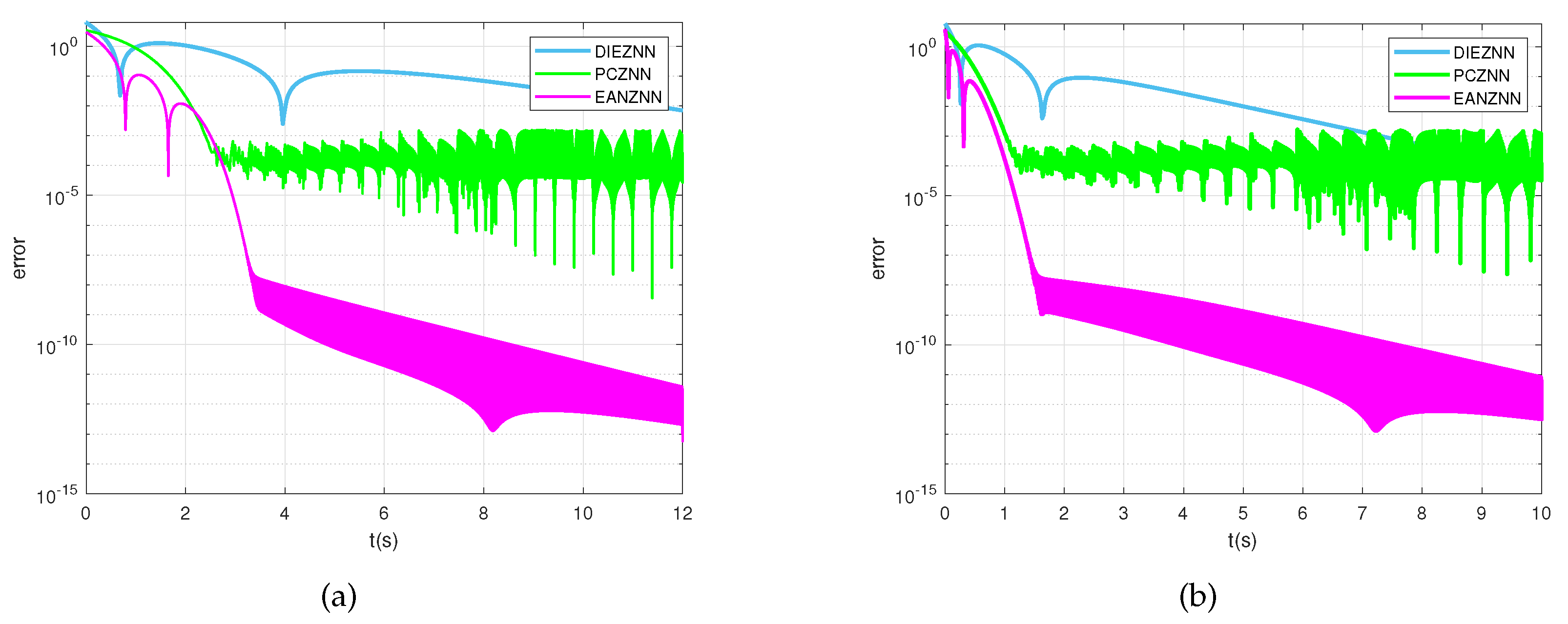
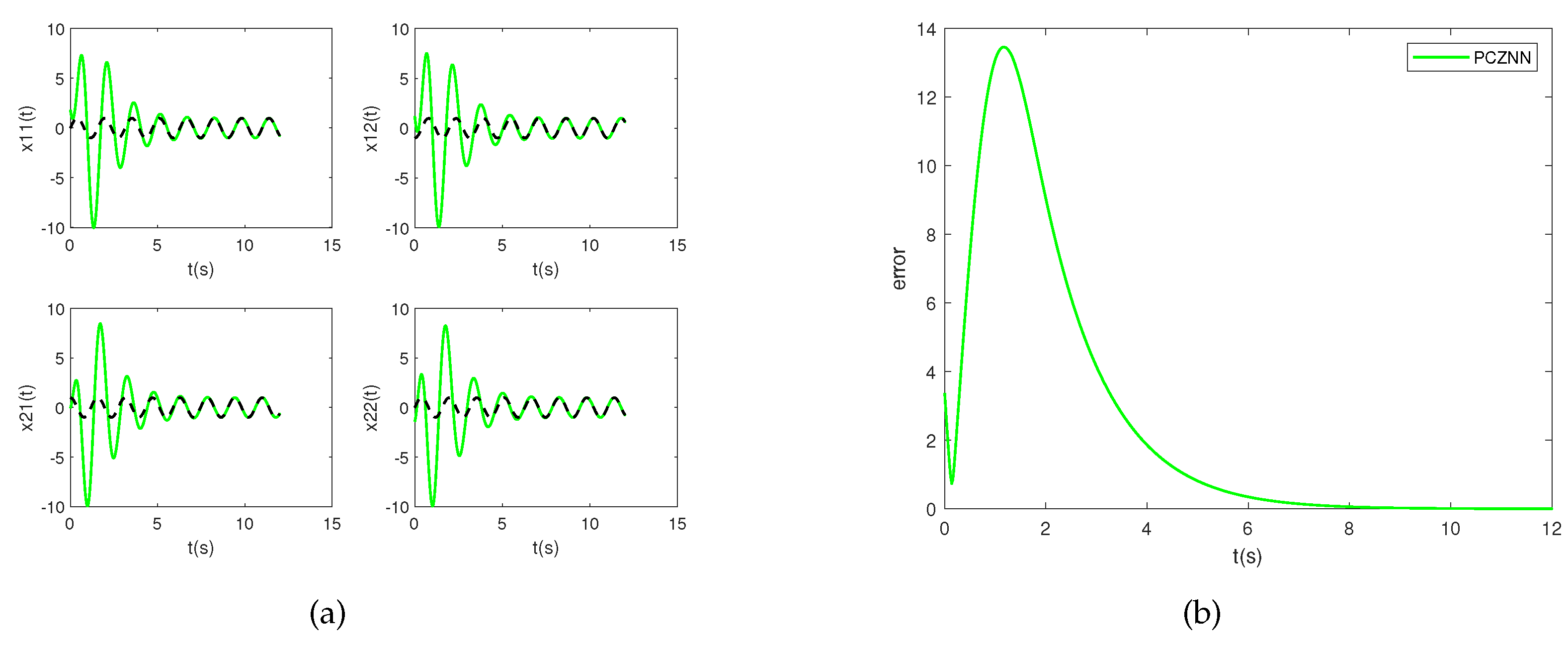
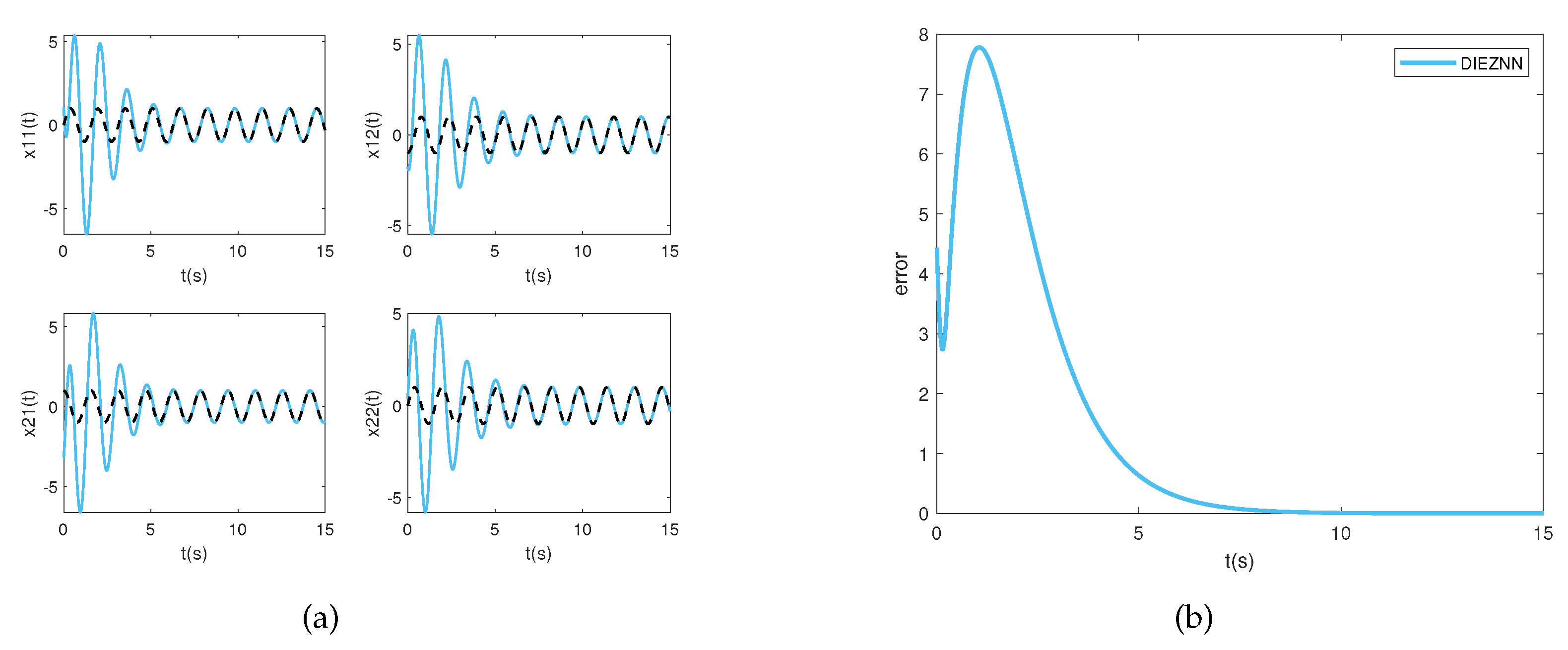
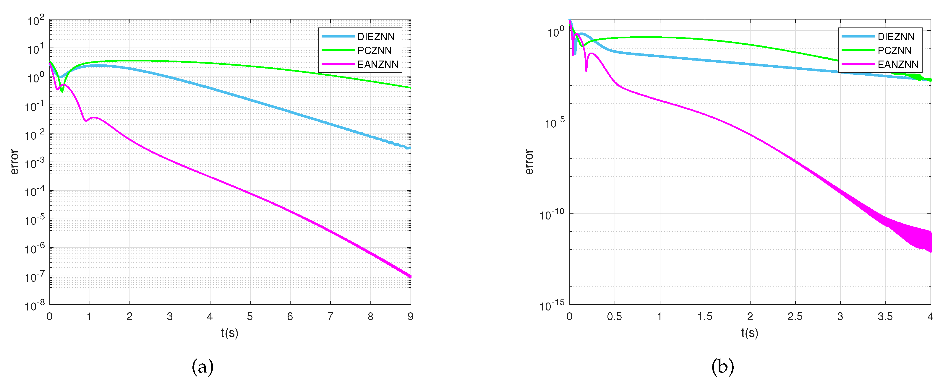
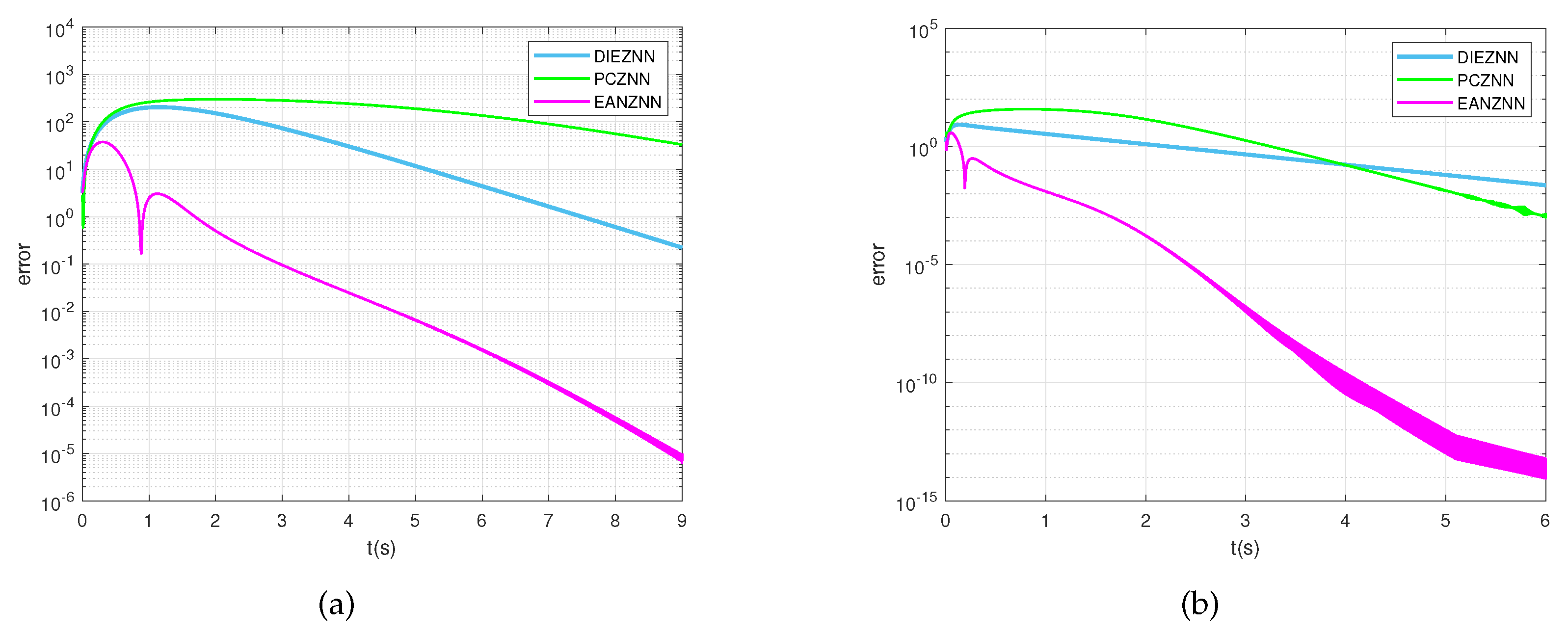
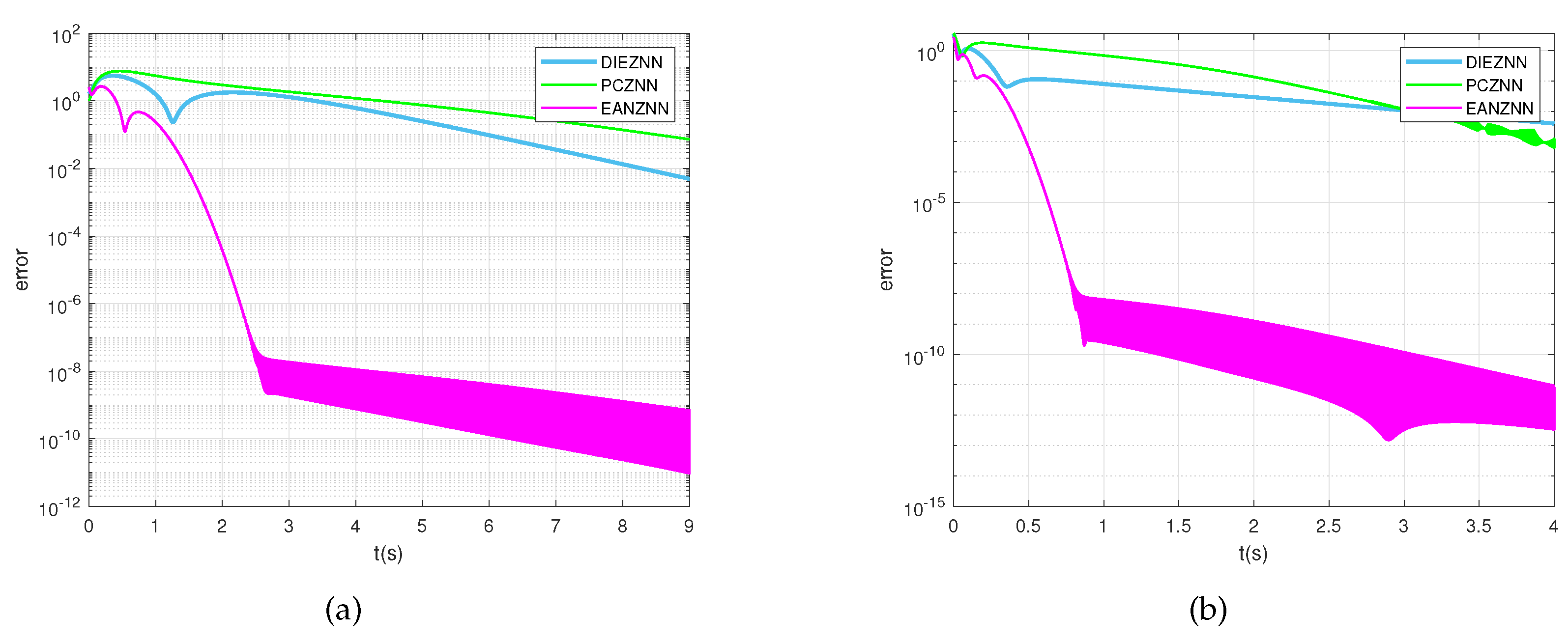
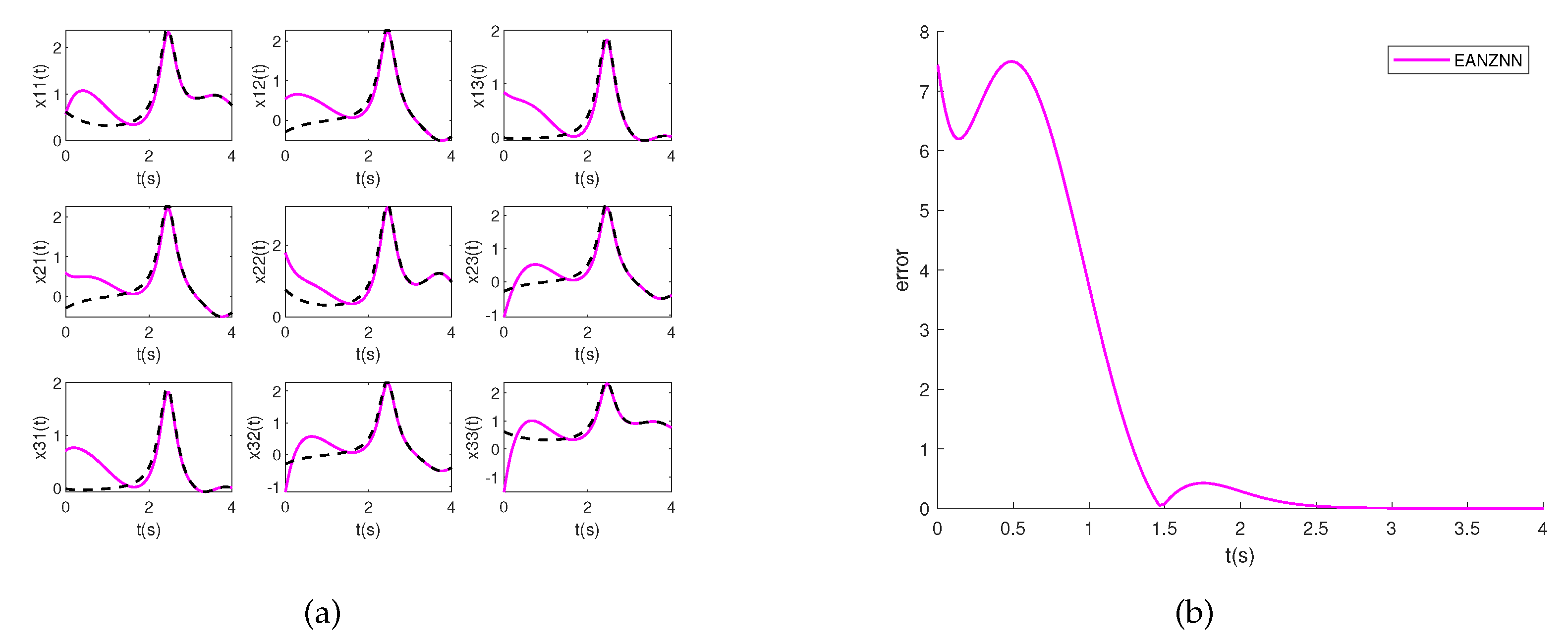
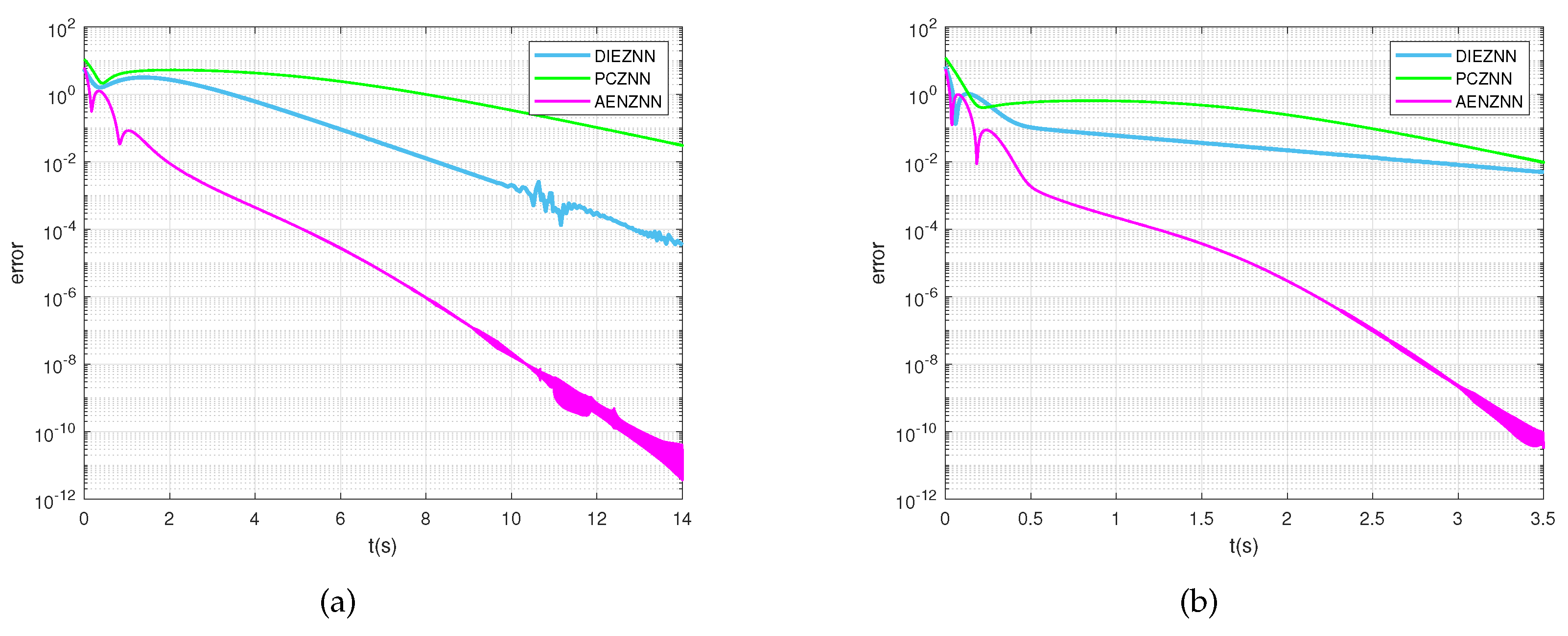
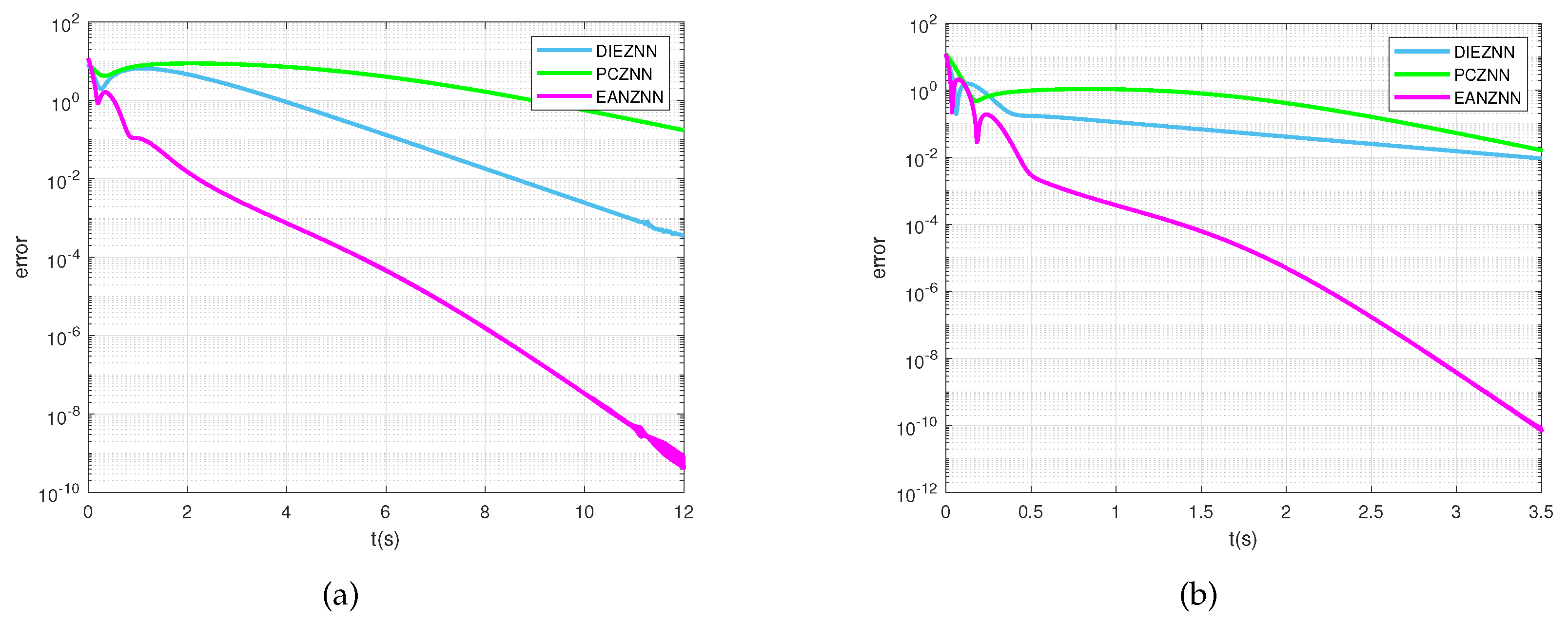
Experimental results show that under noise-free conditions, the EANZNN model achieves a faster convergence speed in solving the TVMI issue compared to the DIEZNN and PCZNN models. Under constant and linear noise conditions, the EANZNN model not only converges faster but also demonstrates superior robustness.

2. TVMI Description and Model Design

This section describes the time-varying matrix inversion (TVMI) problem. Subsequently, it introduces the relevant models and elaborates on the design process of the EANZNN model, which includes double integral terms. The importance of this paper stems from our proposed EANZNN model’s ability to efficiently and precisely solve the TVMI problem.

2.1. Description of TVMI

The TVMI problem can be mathematically formulated as follows:

$$A\left(t\right)U\left(t\right)=I\in {\mathbb{R}}^{n\times n},\mathrm{or}U\left(t\right)A\left(t\right)=I,$$

(1)

where $A\left(t\right)\in {\mathbb{R}}^{n\times n}$ represents a known time-varying, non-singular, smooth coefficient matrix; $U\left(t\right)\in {\mathbb{R}}^{n\times n}$ stands for an unknown invertible matrix; and I signifies a unit matrix of suitable dimensions. The aim of this paper is to use the designed model to solve for $U\left(t\right)$ in Equation (1), with the theoretical solution of $U^{*}\left(t\right)=A^{-1}\left(t\right)\in {\mathbb{R}}^{n\times n}$.

2.2. Relevant Model Design

A ZNN, as a specialized type of recurrent neural network, is typically used to address time-varying problems. Its design process can generally be divided into the following three steps [33]:

• First, define an appropriate error function based on the specific problem to be solved;
• Design an evolution formula that ensures the error function converges to zero;
• Substitute the defined error function into the evolution formula to obtain the corresponding ZNN model.

According to the design steps of the ZNN, to solve the online TVMI problem (1), we first define the error function for TVMI (1) as follows:

$$E\left(t\right)=A\left(t\right)U\left(t\right)-I.$$

(2)

To ensure the convergence of $A\left(t\right)$ towards its theoretical inverse denoted by $U^{-1}\left(t\right)$, it is necessary for the error function ($E\left(t\right)\in {\mathbb{R}}^{n\times n}$) to iteratively approach zero, meaning that each element of the error function is $e_{ij}\left(t\right)\to 0$ for all $i,j\in \{1,\cdots ,n\}$. To achieve this goal and improve the model’s performance, Xiao et al. [32] designed a method using power-type time-varying parameters instead of traditional fixed parameters. Compared to fixed parameters, this design achieves super-exponential convergence and accelerates the convergence speed. Due to $t\in [0,+\infty ]$, the design formula is expressed as follows:

$$\dot{E}\left(t\right)=-\lambda \left(t\right)E\left(t\right),$$

(3)

and the time-varying parameter ($\lambda \left(t\right)$) is defined as

$$\lambda \left(t\right)=\left\{\begin{array}{cc}p{e}^t,\hfill & \hfill 0<p\le 1\\ p^t+2pt+p,\hfill & \hfill p>1.\end{array}\right.$$

(4)

Next, the time derivative of $E\left(t\right)$ in Equation (2) is computed to obtain $\dot{E}\left(t\right)=\dot{A}\left(t\right)U\left(t\right)+A\left(t\right)\dot{U}\left(t\right)$. Substituting Equation (2) and $\dot{E}\left(t\right)$ into Equation (3), the PCZNN model proposed by Xiao et al. [32] to solve the TVMI problem is derived as follows:

$$A\left(t\right)\dot{U}\left(t\right)=-\dot{A}\left(t\right)U\left(t\right)-\lambda \left(t\right)(A\left(t\right)U\left(t\right)-I).$$

(5)

In real-world situations, external noise interference is inevitably encountered, often characterized by random noise and linear noise. Therefore, Liao et al. [29] introduced a DIEZNN model with double integration to effectively suppress noise, as outlined below.

$$\begin{array}{cc}\hfill A\left(t\right)U\left(t\right)=& -A\left(t\right)U\left(t\right)-(2u+1)\left(A\right(t\left)U\right(t)-I)\hfill \\ \hfill & -(u^2+2u){\int }_0^t\left(A\right(\sigma \left)U\right(\sigma )-I)d\sigma \hfill \\ \hfill & -u^2{\int }_0^t{\int }_0^{\sigma }\left(A\right(\tau \left)U\right(\tau )-I)d\tau d\sigma .\hfill \end{array}$$

(6)

Please note that $u>0$ is a parameter used to adjust the convergence speed.

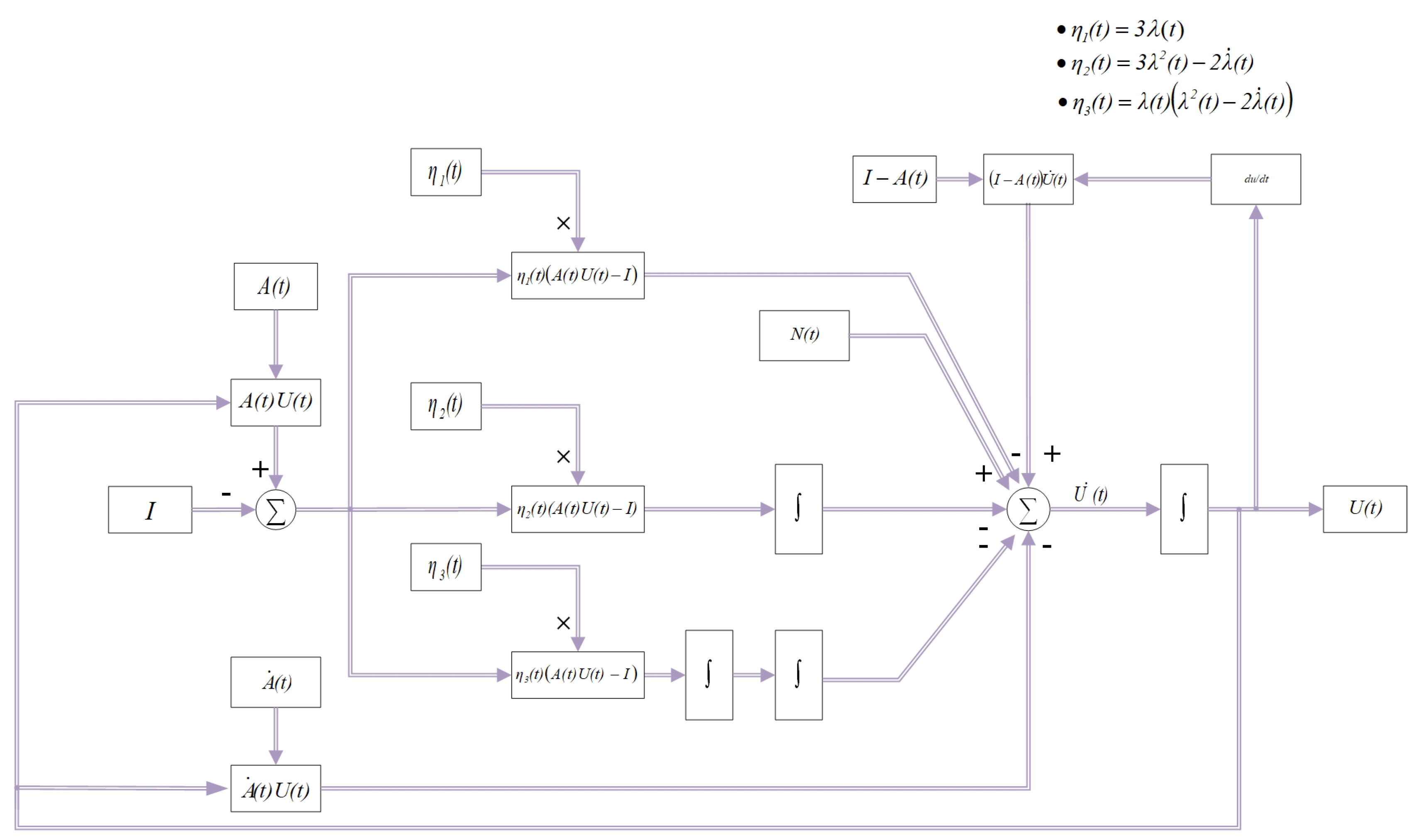
2.3. EANZNN Model Design

In this section, a novel efficient anti-noise zeroing neural network (EANZNN) model is proposed. To track the inversion process, we initially establish an error function that mirrors the one defined in Equation (2). On this basis, inspired by the design methodology detailed in references [32,34], we design the error function ($Y\left(t\right)$) to satisfy the following two equations:

$$\left\{\begin{array}{c}Y\left(t\right)=\dot{E}\left(t\right)+\lambda \left(t\right)E\left(t\right),\hfill \\ Y\left(t\right)=-{\int }_0^t\lambda \left(\sigma \right)Y\left(\sigma \right)d\sigma .\hfill \end{array}\right.$$

(7)

If the time-varying design parameter ($\lambda \left(t\right)$) continues to increase, it may exceed the feasible range or the target limits, which may lead to solution failure. To address this issue, an upper bound is established for the growth of $\lambda \left(t\right)$. Specifically, once t exceeds $t_0$, $\lambda \left(t\right)$ is fixed at a constant value ($\lambda \left(t_0\right)$) no longer increases with t. The explicit definition of $\lambda \left(t\right)$ is provided below.

$$\lambda \left(t\right)=\left\{\begin{array}{cc}p{e}^t,\hfill & \mathrm{if}0<p\le 1\mathrm{and}t\le t_0,\hfill \\ p^t+2pt+p,\hfill & \mathrm{if}p>1\mathrm{and}t\le t_0,\hfill \\ \lambda \left(t_0\right),\hfill & \mathrm{if}t>t_0.\hfill \end{array}\right.$$

(8)

where $t_0$ is defined as 20 s in this document.

Combining the above equations, it can be further deduced that

$$\begin{array}{cc}\hfill Y\left(t\right)& =\dot{E}\left(t\right)+\lambda \left(t\right)E\left(t\right)\hfill \\ \hfill & =-{\int }_0^t\lambda \left(\sigma \right)\left(\dot{E}\left(\sigma \right)+\lambda \left(\sigma \right)E\left(\sigma \right)\right)d\sigma \hfill \\ \hfill & =-\lambda \left(t\right)E\left(t\right)-{\int }_0^t({\lambda }^2\left(\sigma \right)-\dot{\lambda }\left(\sigma \right))E\left(\sigma \right)d\sigma .\hfill \end{array}$$

(9)

Equation (9) is restated as

$$\dot{E}\left(t\right)=-2\lambda \left(t\right)E\left(t\right)-{\int }_0^t({\lambda }^2\left(\sigma \right)-\dot{\lambda }\left(\sigma \right))E\left(\sigma \right)d\sigma .$$

(10)

Similarly to the error function ($Y\left(t\right)$), we can construct the new error function ($G\left(t\right)$) as

$$\left\{\begin{array}{c}G\left(t\right)=\dot{E}\left(t\right)+2\lambda \left(t\right)E\left(t\right)+{\int }_0^t({\lambda }^2\left(\sigma \right)-\dot{\lambda }\left(\sigma \right))E\left(\sigma \right)d\sigma ,\hfill \\ G\left(t\right)=-{\int }_0^t\lambda \left(\sigma \right)G\left(\sigma \right)d\sigma ,\hfill \end{array}\right.$$

(11)

similarly obtaining

$$\begin{array}{cc}\hfill \dot{E}\left(t\right)& +2\lambda \left(t\right)E\left(t\right)+{\int }_0^t\left({\lambda }^2\left(\sigma \right)-\dot{\lambda }\left(\sigma \right)\right)E\left(\sigma \right)d\sigma \hfill \\ \hfill & =-{\int }_0^t\lambda \left(\sigma \right)\left(\dot{E}\left(\sigma \right)+2\lambda \left(\sigma \right)E\left(\sigma \right)+{\int }_0^{\sigma }(({\lambda }^2\left(\tau \right)-\dot{\lambda }\left(\tau \right))E\left(\tau \right)d\tau \right)d\sigma \hfill \\ \hfill & =-{\int }_0^t\left(\lambda \left(\sigma \right)\dot{E}\left(\sigma \right)+2{\lambda }^2\left(\sigma \right)E\left(\sigma \right)\right)d\sigma \hfill \\ \hfill & -{\int }_0^t\left(\lambda \left(\sigma \right){\int }_0^{\sigma }({\lambda }^2\left(\tau \right)-\dot{\lambda }\left(\tau \right))E\left(\tau \right)d\tau \right)d\sigma \hfill \\ \hfill & =-\lambda \left(t\right)E\left(t\right)-{\int }_0^t(2{\lambda }^2\left(\sigma \right)-\dot{\lambda }\left(\sigma \right))E\left(\sigma \right)d\sigma \hfill \\ \hfill & -{\int }_0^t{\int }_0^{\sigma }\lambda \left(\sigma \right)\left(({\lambda }^2\left(\tau \right)-\dot{\lambda }\left(\tau \right))E\left(\tau \right)\right)d\tau d\sigma .\hfill \end{array}$$

(12)

Therefore, we obtain the design of the EANZNN model as follows:

$$\begin{array}{cc}\hfill \dot{E}\left(t\right)=& -3\lambda \left(t\right)E\left(t\right)-{\int }_0^t(3{\lambda }^2\left(\sigma \right)-2\dot{\lambda }\left(\sigma \right))E\left(\sigma \right)d\sigma \hfill \\ \hfill & -{\int }_0^t{\int }_0^{\sigma }\lambda \left(\sigma \right)\left(({\lambda }^2\left(\tau \right)-\dot{\lambda }\left(\tau \right))E\left(\tau \right)\right)d\tau d\sigma .\hfill \end{array}$$

(13)

Additionally, under the influence of noise, the design formula for EANZNN is given by

$$\begin{array}{cc}\hfill \dot{E}\left(t\right)=& -3\lambda \left(t\right)E\left(t\right)-{\int }_0^t(3{\lambda }^2\left(\sigma \right)-2\dot{\lambda }\left(\sigma \right))E\left(\sigma \right)d\sigma \hfill \\ \hfill & -{\int }_0^t{\int }_0^{\sigma }\lambda \left(\sigma \right)\left(({\lambda }^2\left(\tau \right)-\dot{\lambda }\left(\tau \right))E\left(\tau \right)\right)d\tau d\sigma +N\left(t\right),\hfill \end{array}$$

(14)

where $N\left(t\right)\in {\mathbb{R}}^{n\times n}$ represents external noise.

Finally, we incorporate the time derivative of $E\left(t\right)$ into Equation (14) to obtain the design formulation of EANZNN.

$$\begin{array}{cc}\hfill A\left(t\right)\dot{U}\left(t\right)=& -\dot{A}\left(t\right)U\left(t\right)-3\lambda \left(t\right)\left(A\left(t\right)U\left(t\right)-I\right)\hfill \\ \hfill & -{\int }_0^t\left(3{\lambda }^2\left(\sigma \right)-2\dot{\lambda }\left(\sigma \right)\right)(A\left(\sigma \right)U\left(\sigma \right)-I)d\sigma \hfill \\ \hfill & -{\int }_0^t{\int }_0^{\sigma }\lambda \left(\sigma \right)\left(({\lambda }^2\left(\tau \right)-\dot{\lambda }\left(\tau \right))\left(A\left(\tau \right)U\left(\tau \right)-I\right)\right)d\tau d\sigma +N\left(t\right).\hfill \end{array}$$

(15)

By transforming Equation (15), we can obtain the block-diagram form of the noise-disturbed EANZNN model (15) as follows:

$$\begin{array}{cc}\hfill \dot{U}\left(t\right)& =(I-A\left(t\right))\dot{U}\left(t\right)-\dot{A}\left(t\right)U\left(t\right)-3\lambda \left(t\right)\left(A\left(t\right)U\left(t\right)-I\right)\hfill \\ \hfill & -{\int }_0^t\left(3{\lambda }^2\left(\sigma \right)-2\dot{\lambda }\left(\sigma \right)\right)(A\left(\sigma \right)U\left(\sigma \right)-I)d\sigma \hfill \\ \hfill & -{\int }_0^t{\int }_0^{\sigma }\lambda \left(\sigma \right)\left(({\lambda }^2\left(\tau \right)-\dot{\lambda }\left(\tau \right))\left(A\left(\tau \right)U\left(\tau \right)-I\right)\right)d\tau d\sigma +N\left(t\right).\hfill \end{array}$$

(16)

where $A\left(t\right)$ and $\dot{A}\left(t\right)$ are the system inputs; ${\eta }_1\left(t\right)$, ${\eta }_2\left(t\right)$, and ${\eta }_3\left(t\right)$ represent $3\lambda \left(t\right)$, $3{\lambda }^2\left(t\right)-\dot{2\lambda }\left(t\right)$, and $\lambda \left(t\right)\left({\lambda }^2\left(t\right)-\dot{\lambda }\left(t\right)\right)$ respectively; $N\left(t\right)$ denotes external noise; and $U\left(t\right)$ is the state variable. In robotic control systems, the time-varying matrix inversion problem frequently arises in tasks such as motion control, path planning, and state estimation within dynamic environments. In practical applications, robots need to solve the matrix inverse in real time to accurately execute control commands. However, due to factors such as sensor noise, environmental interference, and computational errors, directly solving the matrix inverse can be challenging. The ZNN model effectively handles time-varying problems by updating the inverse matrix in real time, ensuring timely responses of the robotic control system, even in the presence of noise interference. As shown in Figure 1, the EANZNN model with noise interference can be implemented using summators, multipliers, amplifiers, and integrators to solve $U\left(t\right)$.

Figure 1. Structure diagram of the EANZNN model (15) for handling noise interference in the TVMI problem.

3. Theoretical Analyses

Theoretical analysis is conducted to examine the convergence and robustness of the EANZNN model (15) with respect to the TVMI problem (Equation (1)), and the following theoretical proof process is provided.

3.1. Convergence

In the primary theoretical analysis, we explore how well the EANZNN model (15) converges when operating in an ideal noise-free setting.

Theorem 1.

Given a matrix ($A\left(t\right)\in {\mathbb{R}}^{n\times n}$), when the EANZNN model (15) resolves the TVMI problem (1) in a noise-free scenario, the state matrix ($U\left(t\right)\in {\mathbb{R}}^{n\times n}$) converges from the initial state ($U\left(0\right)\in {\mathbb{R}}^{n\times n}$) to the theoretical inverse ($A^{-1}\left(t\right)\in {\mathbb{R}}^{n\times n}$). Specifically, as $t\to \infty$, the error norm ${\parallel E\left(t\right)\parallel }_F$ tends to zero.

Proof. 

According to Section 2.3, we have

$$\left\{\begin{array}{c}G\left(t\right)=-{\int }_0^t\lambda \left(\sigma \right)G\left(\sigma \right)d\sigma ,\hfill \\ \dot{G}\left(t\right)=-\lambda \left(t\right)G\left(t\right).\hfill \end{array}\right.$$

Its element-wise form is

$$\left\{\begin{array}{c}{g}_{ij}\left(t\right)=-{\int }_0^t\lambda \left(\sigma \right)g_{ij}\left(\sigma \right)d\sigma ,\hfill \\ {\dot{g}}_{ij}\left(t\right)=-\lambda \left(t\right)g_{ij}\left(t\right).\hfill \end{array}\right.$$

(17)

We design a Lyapunov function as

$$v\left(t\right)=g_{ij}^2\left(t\right)>0.$$

Combining Equation (17) (${\dot{g}}_{ij}\left(t\right)=-\lambda \left(t\right)g_{ij}\left(t\right)$), we obtain

$$\dot{v}\left(t\right)=2g_{ij}\left(t\right){\dot{g}}_{ij}\left(t\right)=-2\lambda \left(t\right)g_{ij}^2\left(t\right).$$

According to the expression of the design parameter ($\lambda \left(t\right)$) presented in Section 2.3, it is known that when $t\in [0,+\infty ]$, we have $\lambda \left(t\right)>0$. As a result, we obtain $\dot{v}\left(t\right)<0$. Since $v\left(t\right)$ is positive and definite and $\dot{v}\left(t\right)$ is negative and definite, based on the Lyapunov’s asymptotic stability theory [35], we can obtain

$$\underset{t\to \infty }{lim}\left|g_{ij}\left(t\right)\right|=0.$$

(18)

Similarly, based on the expression for the design parameter ($\lambda \left(t\right)$) described in Section 2.3, it is known that as $t\ge t_0$, $\lambda \left(t\right)$ is fixed at a constant value, which we denote as $\omega$. Given that ${\dot{g}}_{ij}\left(t\right)=-\lambda \left(t\right)g_{ij}\left(t\right)$, we can deduce the following:

$$\underset{t\to \infty }{lim}|{\dot{g}}_{ij}\left(t\right)|=\underset{t\to \infty }{lim}|-\omega g_{ij}\left(t\right)|=0.$$

(19)

The elemental form of $Y\left(t\right)$ in Equation (7) is expressed as $y_{ij}\left(t\right)={\dot{e}}_{ij}\left(t\right)+\lambda \left(t\right)e_{ij}\left(t\right)$, where $y_{ij}$ and $e_{ij}$ denote the $ij$th elements of $Y\left(t\right)$ and $E\left(t\right)$, respectively. Similarly, the element-wise form of $G\left(t\right)$ in Equation (11) is $g_{ij}\left(t\right)={\dot{e}}_{ij}\left(t\right)+2\lambda \left(t\right)e_{ij}\left(t\right)+{\int }_0^t({\lambda }^2\left(\sigma \right)-\dot{\lambda }\left(\sigma \right))e_{ij}\left(\sigma \right)d\sigma$. From these equations, we obtain

$$g_{ij}\left(t\right)=y_{ij}\left(t\right)+{\int }_0^t\lambda \left(\sigma \right)y_{ij}\left(\sigma \right)d\sigma .$$

Then, we derive the above equation to obtain

$${\dot{g}}_{ij}\left(t\right)={\dot{y}}_{ij}\left(t\right)+\lambda \left(t\right)y_{ij}\left(t\right).$$

Given that $\lambda \left(t\right)$ is fixed at a constant value ($\omega$) for $t\ge t_0$, as $t\to \infty$, we can derive the following equivalent substitution from Equation (19):

$$\underset{t\to \infty }{lim}\left|{\dot{y}}_{ij}\left(t\right)+\omega y_{ij}\left(t\right)\right|=0.$$

(20)

Based on Equation (20), we can deduce the following:

$$\underset{t\to \infty }{lim}\left|{\dot{y}}_{ij}\left(t\right)\right|=\underset{t\to \infty }{lim}\left|-\omega y_{ij}\left(t\right)\right|.$$

We establish the following Lyapunov function:

$$s\left(t\right)=y_{ij}^2\left(t\right)>0.$$

Differentiating the equation provided above, we obtain

$$\dot{s}\left(t\right)=2y_{ij}\left(t\right){\dot{y}}_{ij}\left(t\right)=-2\omega y_{ij}^2\left(t\right)<0.$$

As $t\to \infty$, it can be known that $s\left(t\right)$ is positive and definite and $\dot{s}\left(t\right)$ is negative and definite. Based on Lyapunov’s asymptotic stability theory, we can obtain

$$\underset{t\to \infty }{lim}\left|y_{ij}\left(t\right)\right|=0.$$

(21)

Subsequently, substituting the expression $y_{ij}\left(t\right)={\dot{e}}_{ij}\left(t\right)+\lambda \left(t\right)e_{ij}\left(t\right)$ from Equation (21) yields the following equation:

$$\underset{t\to \infty }{lim}|{\dot{e}}_{ij}\left(t\right)+\omega e_{ij}\left(t\right)|=0.$$

(22)

Therefore, we have

$$\underset{t\to \infty }{lim}\left|{\dot{e}}_{ij}\left(t\right)\right|=\underset{t\to \infty }{lim}\left|-\omega e_{ij}\left(t\right)\right|.$$

Following the same method, we define the following Lyapunov function:

$$h\left(t\right)=e_{ij}^2\left(t\right)>0.$$

By differentiating the preceding equation, we obtain

$$\dot{h}\left(t\right)=2e_{ij}\left(t\right){\dot{e}}_{ij}\left(t\right)=-2\omega e_{ij}^2\left(t\right)<0.$$

Similarly, as $t\to \infty$, it can be known that $h\left(t\right)$ is positive and definite and $\dot{h}\left(t\right)$ is negative and definite. Based on Lyapunov’s theory of asymptotic stability, it follows that

$$\underset{t\to \infty }{lim}\left|e_{ij}\left(t\right)\right|=0.$$

Since $\underset{t\to \infty }{lim}\left|e_{ij}\left(t\right)\right|=0$, its corresponding matrix form can also be expressed as

$$\underset{t\to \infty }{lim}{\parallel E\left(t\right)\parallel }_F=0.$$

As a result, the demonstration is finished.  □

3.2. Robustness

In practical scenarios, external noise interference is common and nearly unavoidable. Therefore, it is essential to consider its impact. This section investigates the robustness of the EANZNN model (15) under the interference of matrix-type external noise ($N\left(t\right)$).

Theorem 2.

Given a matrix ($A\left(t\right)\in {\mathbb{R}}^{n\times n}$), when the EANZNN model (15) resolves the TVMI problem (1) under the interference of external constant matrix-type noise ($N\left(t\right)=K\in {\mathbb{R}}^{n\times n}$), the state matrix ($U\left(t\right)\in {\mathbb{R}}^{n\times n}$) converges from the initial state ($U\left(0\right)\in {\mathbb{R}}^{n\times n}$) to the theoretical inverse ($A^{-1}\left(t\right)\in {\mathbb{R}}^{n\times n}$). Specifically, as $t\to \infty$, the error norm (${\parallel E\left(t\right)\parallel }_F$) tends to zero.

Proof. 

The noise ($N\left(t\right)$) is specified by

$$N\left(t\right)=K,$$

where $K\in {\mathbb{R}}^{n\times n}$ is a constant matrix, and the form of the corresponding element is

$$n_{ij}\left(t\right)=k_{ij}.$$

Considering the noise ($N\left(t\right)$) described in Equation (15), we have

$$\left\{\begin{array}{c}{g}_{ij}\left(t\right)=-{\int }_0^t\lambda \left(\sigma \right)g_{ij}\left(\sigma \right)d\sigma +n_{ij}\left(t\right),\hfill \\ {\dot{g}}_{ij}\left(t\right)=-\lambda \left(t\right)g_{ij}\left(t\right)+{\dot{n}}_{ij}\left(t\right).\hfill \end{array}\right.$$

By differentiating $n_{ij}\left(t\right)$, we find

$${\dot{n}}_{ij}\left(t\right)=0.$$

Therefore, we have

$$\left\{\begin{array}{c}{g}_{ij}\left(t\right)=-{\int }_0^t\lambda \left(\sigma \right)g_{ij}\left(\sigma \right)d\sigma +k_{ij}\left(t\right),\hfill \\ {\dot{g}}_{ij}\left(t\right)=-\lambda \left(t\right)g_{ij}\left(t\right).\hfill \end{array}\right.$$

(23)

Similar to the derivation of Equation (18), we conclude that

$$\underset{t\to \infty }{lim}\left|g_{ij}\left(t\right)\right|=0.$$

Similarly, considering that Equation (23) includes ${\dot{g}}_{ij}\left(t\right)=-\lambda \left(t\right)g_{ij}\left(t\right)$, we have

$$\underset{t\to \infty }{lim}\left|{\dot{g}}_{ij}\left(t\right)\right|=\underset{t\to \infty }{lim}\left|-\omega g_{ij}\left(t\right)\right|=0.$$

(24)

Given that Equation (24) is identical to Equation (19), it can be deduced that

$$\underset{t\to \infty }{lim}\left|y_{ij}\left(t\right)\right|=0,$$

(25)

due to

$$y_{ij}\left(t\right)={\dot{e}}_{ij}\left(t\right)+\lambda \left(t\right)e_{ij}\left(t\right).$$

Consequently, substituting this expression into Equation (25), we derive

$$\underset{t\to \infty }{lim}|{\dot{e}}_{ij}\left(t\right)+\omega e_{ij}\left(t\right)|=0.$$

Since the aforementioned equation is identical to Equation (22), we obtain

$$\underset{t\to \infty }{lim}\left|e_{ij}\left(t\right)\right|=0.$$

The corresponding matrix form is written as follows:

$$\underset{t\to \infty }{lim}{\parallel E\left(t\right)\parallel }_F=0.$$

As a result, the demonstration is finished.  □

Theorem 3.

Given a matrix ($A\left(t\right)\in {\mathbb{R}}^{n\times n}$), when the EANZNN model (15) resolves the TVMI problem (1) under the interference of linear noise ($N\left(t\right)=Kt+B\in {\mathbb{R}}^{n\times n}$), the state matrix ($U\left(t\right)\in {\mathbb{R}}^{n\times n}$) converges from the initial state ($U\left(0\right)\in {\mathbb{R}}^{n\times n}$) to the theoretical inverse ($A^{-1}\left(t\right)\in {\mathbb{R}}^{n\times n}$). Specifically, as $t\to \infty$, the error norm (${\parallel E\left(t\right)\parallel }_F$) tends to zero.

Proof. 

The noise ($N\left(t\right)$) is specified by

$$N\left(t\right)=Kt+B,$$

where $K,B\in {\mathbb{R}}^{n\times n}$ represents constant matrices, and their corresponding elemental forms are represented as

$$n_{ij}\left(t\right)=k_{ij}t+b_{ij}.$$

Considering the linear noise ($N\left(t\right)$) described in Equation (15), we have

$$\left\{\begin{array}{c}{g}_{ij}\left(t\right)=-{\int }_0^t\lambda \left(\sigma \right)g_{ij}\left(\sigma \right)d\sigma +n_{ij}\left(t\right),\hfill \\ {\dot{g}}_{ij}\left(t\right)=-\lambda \left(t\right)g_{ij}\left(t\right)+{\dot{n}}_{ij}\left(t\right).\hfill \end{array}\right.$$

Taking the derivative of $n_{ij}\left(t\right)$, we obtain

$${\dot{n}}_{ij}\left(t\right)=k_{ij}.$$

Therefore, we obtain

$$\left\{\begin{array}{c}{g}_{ij}\left(t\right)=-{\int }_0^t\lambda \left(\sigma \right)g_{ij}\left(\sigma \right)d\sigma +n_{ij}\left(t\right),\hfill \\ {\dot{g}}_{ij}\left(t\right)=-\lambda \left(t\right)g_{ij}\left(t\right)+k_{ij}.\hfill \end{array}\right.$$

(26)

To analyze the limit ($\underset{t\to \infty }{lim}\left|{\dot{g}}_{ij}\left(t\right)\right|$) and considering that as $t\to \infty$, $\lambda \left(t\right)$ is fixed at a constant value ($\omega$) for $t\ge t_0$, we can rewrite Equation (26) as

$$\left\{\begin{array}{c}{g}_{ij}\left(t\right)=-{\int }_0^t\omega g_{ij}\left(\sigma \right)d\sigma +n_{ij}\left(t\right),\hfill \\ {\dot{g}}_{ij}\left(t\right)=-\omega g_{ij}\left(t\right)+k_{ij}.\hfill \end{array}\right.$$

After differentiating the expression for ${\dot{g}}_{ij}\left(t\right)$ in the aforementioned equation once again, we obtain the following result:

$${\ddot{g}}_{ij}\left(t\right)=-\omega {\dot{g}}_{ij}\left(t\right).$$

We define the following Lyapunov function:

$$\theta \left(t\right)={\dot{g}}_{ij}^2\left(t\right)>0.$$

Differentiating the above expression, we obtain

$$\dot{\theta }\left(t\right)=2{\dot{g}}_{ij}\left(t\right){\ddot{g}}_{ij}\left(t\right)=-2\omega {\dot{g}}_{ij}^2\left(t\right)<0.$$

As $t\to \infty$, $\theta \left(t\right)$ is positive and definite, and $\dot{\theta }\left(t\right)$ is negative and definite. According to Lyapunov’s theorem of asymptotic stability, we can derive

$$\underset{t\to \infty }{lim}\left|{\dot{g}}_{ij}\left(t\right)\right|=0.$$

Substituting $g_{ij}\left(t\right)=y_{ij}\left(t\right)+{\int }_0^t\lambda \left(\sigma \right)y_{ij}\left(\sigma \right)d\sigma$ into the above equation, we further obtain

$$\underset{t\to \infty }{lim}|{\dot{y}}_{ij}\left(t\right)+\omega y_{ij}\left(t\right)|=0.$$

(27)

Noting that Equation (27) is identical to Equation (20), we can infer

$$\underset{t\to \infty }{lim}\left|y_{ij}\left(t\right)\right|=0.$$

Since $y\left(t\right)={\dot{e}}_{ij}\left(t\right)+\lambda \left(t\right)e_{ij}\left(t\right)$,

$$\underset{t\to \infty }{lim}|{\dot{e}}_{ij}\left(t\right)+\omega e_{ij}\left(t\right)|=0.$$

This equation is similar to Equation (22), from which it follows that

$$\underset{t\to \infty }{lim}\left|e_{ij}\left(t\right)\right|=0.$$

The corresponding matrix form is written as follows:

$$\underset{t\to \infty }{lim}{\parallel E\left(t\right)\parallel }_F=0.$$

As a result, the demonstration is finished.  □

4. Example Verification

Remark 1.

The experimental data and results presented in this paper were obtained using MATLAB R2021a Version. Initially, the EANZNN model (15) was built in MATLAB, where the design parameter (p) was set, and the initial state matrix ($U\left(0\right)$) was randomly generated to handle the given time-varying matrix ($A\left(t\right)$). Next, the matrix differential equation was converted into a vector differential equation using the "kron" function (Kronecker product technique) in Matlab, followed by solving the differential equation using the ode45 solver. Through iterative updates, the dynamic system outputs the real-time state solution ($U\left(t\right)$). Additionally, the Frobenius norm (${\Vert ·\Vert }_F$) was calculated to obtain real-time data and results of the error function ($E\left(t\right)$).

In this section, we further verify the effectiveness and superiority of the EANZNN model (15) in solving the TVMI problem (1) under noise-free and external noise conditions through three examples. To clearly demonstrate the experimental results and the advantages of the EANZNN model (15), we also compared it with the existing PCZNN model (5) and DIEZNN model (6) under the same conditions, considering the results with different design parameters ($u=p=0.8$, $u=p=2$, $u=p=3$, and $u=p=15$). These simulations were all conducted on a laptop equipped with a Windows 10 64-bit operating system, Intel Core i7-11800H CPU (2.30 GHz), and 16 GB of memory.

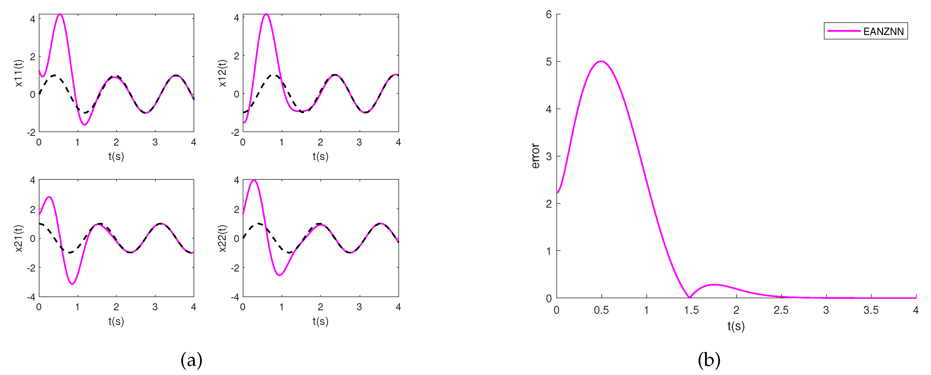
4.1. Experiment 1—Convergence

To validate the effectiveness and convergence of the EANZNN model in solving the TVMI problem, we used simple 2 × 2 time-varying coefficient matrices ($A\left(t\right)$) (28), with random initial values ($U\left(0\right)$) and various design parameters. In the experiment, we conducted a comparative analysis of the EANZNN model relative to the PCZNN and DIEZNN models under noise-free conditions.

We considered the following time-varying invertible matrix ($A\left(t\right)$) for the TVMI problem:

$$A\left(t\right)=\left[\begin{array}{cc}sin\left(4t\right)& cos\left(4t\right)\\ -cos\left(4t\right)& sin\left(4t\right)\end{array}\right]\in {\mathbb{R}}^{2\times 2}.$$

(28)

Obviously, the theoretical solution ($U^{*}\left(t\right)$) of the corresponding TVMI can be readily computed as

$$U^{*}\left(t\right)=A^{-1}\left(t\right)=\left[\begin{array}{cc}sin\left(4t\right)& -cos\left(4t\right)\\ cos\left(4t\right)& sin\left(4t\right)\end{array}\right]\in {\mathbb{R}}^{2\times 2}.$$

This inverse serves as a benchmark to evaluate the accuracy of the solutions obtained by the PCZNN, DIEZNN, and EANZNN models for the TVMI problem.

Figure 2 presents the convergence trajectories of the error norm (${\parallel E\left(t\right)\parallel }_F$) when solving the TVMI problem using the PCZNN, DIEZNN, and EANZN models under a noise-free environment. As can be seen, starting from the randomly generated initial state ($U\left(0\right)\in {[-2,2]}^{2\times 2}$), all three models converge to approximately zero. With design parameters of $u=p=0.8$, as illustrated in Figure 2a, the error norm (${\left|\right|E\left(t\right)\left|\right|}_F$) for DIEZNN converges to just above ${10}^{-3}$ within 12 s. PCZNN’s convergence accuracy stabilizes at around ${10}^{-4}$, while EANZNN exhibits higher precision, achieving a convergence accuracy of ${10}^{-5}$ within 3 s and further converging to ${10}^{-11}$ within 12 s. Figure 2b shows the results with design parameters of $u=p=3$. It can be seen that EANZNN significantly outperforms the other two models in terms of convergence speed and precision. Specifically, the error norm (${\left|\right|E\left(t\right)\left|\right|}_F$) for EANZNN rapidly decreases to ${10}^{-3}$ within 1 s and further improves to approximately ${10}^{-13}$ over time. In contrast, PCZNN and DIEZNN only converge to above ${10}^{-8}$ within 10 s. Among them, PCZNN stabilizes around ${10}^{-4}$, while DIEZNN converges above ${10}^{-5}$. These comparative results indicate that the proposed EANZNN model demonstrates significant advantages in noise-free environments, not only achieving faster convergence but also reaching higher convergence accuracy in a shorter time, showcasing its superior performance in handling the TVMI problem.

Figure 2. The error norm (${\left|\right|E\left(t\right)\left|\right|}_F$) computed for the TVMI of the matrix equation (28) using PCZNN, DIEZNN, and EANZNN under noise-free conditions. (a) u = p= 0.8; (b) u = p = 3.

4.2. Experiment 2—Robustness

Next, to verify the robustness and convergence of the EANZNN model, we conducted further experiments under different noise conditions. Specifically, we solved the TVMI problem in the presence of constant and linear noise. We continued using the time-varying matrix ($A\left(t\right)$) (28) defined in the previous experiment and considered different noise intensities and design parameters. Through these experiments, we assessed the performance of the EANZNN model under noise interference and compared it with that of the PCZNN and DIEZNN models.

Although all three models converge under noise-free conditions, it is more important to consider model validation under external noise. Figure 3, Figure 4 and Figure 5 display the convergence trajectories of the state ($U\left(t\right)$) and the error norm (${\left|\right|E\left(t\right)\left|\right|}_F$) synthesized by the PCZNN, DIEZNN, and EANZNN models under linear noise conditions ($N\left(t\right)={[10+10t]}^{2\times 2}$). Here, the symbol ${[10t+10]}^{2\times 2}$ represents a $2\times 2$ matrix where each element is $10t+10$, which was used to simulate the impact of linear noise at different times (t). In these figures, the initial state ($U\left(0\right)$) is randomly generated as $U\left(0\right)\in {[-2,2]}^{2\times 2}$, and the model parameters are set to $u=1$ and $p=1$. The theoretical state solution is depicted by the black dashed line, while the state solutions of the PCZNN, DIEZNN, and EANZNN models are represented by the green solid line, light-blue solid line, and magenta solid line, respectively.

Figure 3. Simulation results of solving the TVMI problem for matrix Equation (28) using PCZNN with $p=1$ under conditions of linear noise ($N\left(t\right)={[10+10t]}^{2\times 2}$). (a) State $U\left(t\right)$; (b) error norm ${\left|\right|E\left(t\right)\left|\right|}_F$.

Figure 4. Simulation results of solving the TVMI problem for matrix Equation (28) using DIEZNN with $u=1$ under conditions of linear noise ($N\left(t\right)={[10+10t]}^{2\times 2}$). (a) State $U\left(t\right)$; (b) error norm ${\left|\right|E\left(t\right)\left|\right|}_F$.

Figure 5. Simulation results of solving the TVMI problem for matrix Equation (28) using EANZNN with $p=1$ under conditions of linear noise ($N\left(t\right)={[10+10t]}^{2\times 2}$). (a) State $U\left(t\right)$; (b) Error norm ${\left|\right|E\left(t\right)\left|\right|}_F$.

Figure 3a displays the state solution, while Figure 3b illustrates the error norm for PCZNN. From Figure 3a, it can be visually observed that under linear noise conditions ($N\left(t\right)={[10+10t]}^{2\times 2}$), PCZNN converges to zero in approximately 12 s. Figure 4a and Figure 4b show the state solution and error norm of DIEZNN, respectively. It can be observed from Figure 4b that DIEZNN converges to zero in approximately 15 s and remains stable under this linear noise.

Figure 5a and Figure 5b depict the state solution and the error norm of EANZNN, respectively. It is evident that EANZNN can converge to zero under linear noise conditions ($N\left(t\right)={[10+10t]}^{2\times 2}$). From Figure 5b, it can be observed that EANZNN converges to zero in approximately 3.5 s with a design parameter of $p=1$ and remains stable under this linear noise. Therefore, it can be concluded from the aforementioned findings that when subjected to linear noise conditions ($N\left(t\right)={[10+10t]}^{2\times 2}$), EANZNN exhibits the shortest computation time to resolve the TVMI problem, showcasing its superior convergence and robustness.

Next, several other external noises ($N\left(t\right)$) were investigated to further illustrate the superior noise suppression performance of EANZNN.

• Linear noise: $N\left(t\right)={[12t+0.8]}^{2\times 2}$;
• Linear noise: $N\left(t\right)={[1000t+100]}^{2\times 2}$;
• Constant noise: $N\left(t\right)={\left[20\right]}^{2\times 2}$.

Figure 6a,b show the error norm (${\left|\right|E\left(t\right)\left|\right|}_F$) when solving the TVMI problem under linear noise conditions ($N\left(t\right)={[12t+0.8]}^{2\times 2}$) using the PCZNN, DIEZNN, and EANZNN models. Figure 6a presents the results for $u=p=2$, where PCZNN does not converge to near zero within 9 s, while DIEZNN converges to approximately $3.12\times {10}^{-3}$ around 9 s. Compared with these two models, EANZNN converges the fastest, with the error norm (${\left|\right|E\left(t\right)\left|\right|}_F$) starting to be less than ${10}^{-5}$ after approximately 6 s. Figure 6b shows the results when the parameters of the three models are $u=p=15$. It is evident that the error norm (${\left|\right|E\left(t\right)\left|\right|}_F$) of EANZNN is less than ${10}^{-5}$ after about 1.8 s, whereas the error norms (${\left|\right|E\left(t\right)\left|\right|}_F$) of the other two models only converge to ${10}^{-3}$ or higher.

Figure 6. Under linear noise ($N\left(t\right)={[12t+0.8]}^{2\times 2}$), the error norm (${\left|\right|E\left(t\right)\left|\right|}_F$) for the TVMI of the matrix equation (28) is computed using PCZNN, DIEZNN, and EANZNN. (a) $u=p=2$; (b) $u=p=15$.

The error norm (${\left|\right|E\left(t\right)\left|\right|}_F$) of PCZNN, DIEZNN, and EANZNN under linear noise conditions ($N\left(t\right)={[1000t+100]}^{2\times 2}$) is shown in Figure 7. Figure 7a presents the results when the parameters of the three models are $u=p=2$. PCZNN does not converge to a near-zero value within 9 s, whereas DIEZNN converges to $2.27\times {10}^{-1}$ within the same time frame and EANZNN converges to ${10}^{-5}$. Figure 7b shows the results when the parameters for the three models are set to $u=p=15$; in comparison, the error norm ${\left|\right|E\left(t\right)\left|\right|}_F$ of EANZNN starts to be less than ${10}^{-7}$ after 3 s, while both PCZNN and DIEZNN do not converge to ${10}^{-5}$ within 3 s. In summary, when the linear noise increases, the convergence performance of EANZNN far surpasses that of DIEZNN and PCZNN.

Figure 7. Under linear noise ($N\left(t\right)={[1000t+100]}^{2\times 2}$), the error norm (${\left|\right|E\left(t\right)\left|\right|}_F$) for the TVMI of the matrix equation (28) is computed using PCZNN, DIEZNN, and EANZNN. (a) $u=p=2$; (b) $u=p=15$.

Furthermore, Figure 8a,b display the error norm (${\left|\right|E\left(t\right)\left|\right|}_F$) of PCZNN, DIEZNN, and EANZNN under constant noise ($N\left(t\right)={\left[20\right]}^{2\times 2}$). As illustrated in Figure 8a, under the influence of constant noise ($N\left(t\right)={\left[20\right]}^{2\times 2}$), for the case of $u=p=2$, the error norm (${\left|\right|E\left(t\right)\left|\right|}_F$) of the EANZNN model rapidly declines and stabilizes below $1.831\times {10}^{-8}$ within approximately 3 s. In contrast, the PCZNN and DIEZNN models do not achieve lower error levels within the 9 s observation period, with error norms only converging to above ${10}^{-3}$. With the increase in design parameters, as shown in Figure 8b, when $u=p=15$, the residuals decrease for all models. However, EANZNN achieves significantly quicker convergence than PCZNN and DIEZNN. Therefore, it is clear that the presented EANZNN exhibits greater convergence performance in resolving the TVMI problem in the presence of constant noise as compared to PCZNN and DIEZNN.

Figure 8. Under linear noise ($N\left(t\right)={\left[20\right]}^{2\times 2}$), the error norm (${\left|\right|E\left(t\right)\left|\right|}_F$) for the TVMI of the matrix equation (28) is computed using PCZNN, DIEZNN, and EANZNN. (a) $u=p=2$; (b) $u=p=15$.

4.3. Experiment 3—High-Dimensional Matrix

In order to further illustrate the efficiency and superiority of the constructed EANZNN in computing the TVMI, we consider the following two high-dimensional example equations:

$$A\left(t\right)=\left[\begin{array}{ccc}2.1+sin\left(1.5t\right)& cos\left(1.5t\right)& {\displaystyle \frac{cos\left(1.5t\right)}{2}}\\ cos\left(1.5t\right)& 2.1+sin\left(1.5t\right)& cos\left(1.5t\right)\\ {\displaystyle \frac{cos\left(1.5t\right)}{2}}& cos\left(1.5t\right)& 2.1+sin\left(1.5t\right)\end{array}\right],$$

(29)

and

$$A\left(t\right)=\left[\begin{array}{ccccc}1.1+sin\left(t\right)& 0.3cos\left(t\right)& 0.2sin\left(2t\right)& 0.1cos\left(2t\right)& 0.2sin\left(t\right)\\ 0.3cos\left(t\right)& 1.2+cos\left(t\right)& 0.3sin\left(t\right)& 0.2cos\left(2t\right)& 0.1sin\left(2t\right)\\ 0.2sin\left(2t\right)& 0.3sin\left(t\right)& 1.3+sin\left(t\right)& 0.1cos\left(t\right)& 0.2cos\left(2t\right)\\ 0.1cos\left(2t\right)& 0.2cos\left(2t\right)& 0.1cos\left(t\right)& 1.4+0.5sin\left(t\right)& 0.3sin\left(2t\right)\\ 0.2sin\left(t\right)& 0.1sin\left(2t\right)& 0.2cos\left(2t\right)& 0.3sin\left(2t\right)& 1.5+cos\left(t\right)\end{array}\right].$$

(30)

Figure 9a illustrates the individual entries of the state solutions ($U\left(t\right)$) of the TVMI problem, which were computed using the EANZNN method. The state solutions of $U\left(t\right)$ all converge to the theoretical solution within a short period of time, as can be observed. Observing Figure 9b, it is noted that the corresponding error norm (${\left|\right|E\left(t\right)\left|\right|}_F$) synthesized by EANZNN converges to zero in approximately 3 s. This further affirms that the performance of the established EANZNN remains unaffected by variations in matrix dimensions during the resolution of the TVMI problem.

Figure 9. Simulation results of solving the TVMI problem for matrix equation (29) using EANZNN with $p=1$ under the conditions of linear noise ($N\left(t\right)={[10+10t]}^{3\times 3}$). (a) State $U\left(t\right)$; (b) Error norm ${\left|\right|E\left(t\right)\left|\right|}_F$.

By observing Figure 10, it can be noted that for the inversion of a high-dimensional matrix (29), when $u=p=2$, the error norm (${\left|\right|E\left(t\right)\left|\right|}_F$) of EANZNN begins to decrease below ${10}^{-10}$ after 10 s. Specifically, both PCZNN and DIEZNN fail to converge to ${10}^{-6}$ within 14 s, with DIEZNN’s error norm reducing to approximately $3.66\times {10}^{-5}$ at 14 s, while PCZNN’s error norm decreases to about $3.19\times {10}^{-2}$ at the same time. Figure 10b also shows that when the parameters are adjusted to $u=p=15$, all models’ error norms (${\left|\right|E\left(t\right)\left|\right|}_F$) are able to converge to nearly zero. However, EANZNN displays the fastest convergence rate, with its error norm dropping below $1\times {10}^{-8}$ within 3 s, whereas the error norms of PCZNN and DIEZNN only converge to above ${10}^{-3}$ within 3.5 s. This confirms the superior convergence performance of EANZNN compared to PCZNN and DIEZNN when addressing the TVMI problem for high-dimensional matrices.

Figure 10. Under the condition of linear noise ($N\left(t\right)={[12t+0.8]}^{3\times 3}$), the error norm (${\left|\right|E\left(t\right)\left|\right|}_F$) for the TVMI of the matrix equation (29) is computed using PCZNN, DIEZNN, and EANZNN. (a) $u=p=2$; (b) $u=p=15$.

Similarly, Figure 11 shows the inversion of high-dimensional matrices (30) under noisy conditions using the PCZNN, DIEZNN, and EANZNN models. As shown in Figure 11a, when $u=p=2$, the error norm (${\Vert E\left(t\right)\Vert }_F$) for PCZNN does not converge to near zero within 12 s. DIEZNN requires 12 s to reach an error norm of ${10}^{-3}$, while EANZNN achieves the same error norm in just 4 s and further reduces the error norm to approximately ${10}^{-10}$ over time. As illustrated in Figure 11b, with increased design parameters $u=p=15$, the convergence speed significantly accelerates. EANZNN reaches an error norm of ${10}^{-11}$ within 3.5 s, whereas PCZNN and DIEZNN only converge to above ${10}^{-2}$ within the same time frame.The experimental results indicate that EANZNN outperforms DIEZNN and PCZNN in terms of convergence speed and accuracy, even under noisy high-dimensional matrix conditions.

Figure 11. Under the condition of linear noise ($N\left(t\right)={[12t+0.8]}^{5\times 5}$), the error norm (${\left|\right|E\left(t\right)\left|\right|}_F$) for the TVMI of the matrix equation (30) is computed using PCZNN, DIEZNN, and EANZNN. (a) $u=p=2$. (b) $u=p=15$.

Based on the simulation results reported above, it is evident that EANZNN demonstrates superior robustness and convergence compared to PCZNN and DIEZNN when tackling the TVMI problem, irrespective of external noise conditions.

5. Conclusions

To effectively address the TVMI problem, we first investigated the design of segmented time-varying parameters. Based on this, we designed an EANZNN model incorporating double integrals. Additionally, we provided rigorous theoretical proofs of the convergence and robustness of EANZNN. Simulation experiments on matrices of different dimensions and under different noise conditions demonstrated that EANZNN achieves quicker convergence and greater resilience to noise than the DIEZNN and PCZNN models. These results unequivocally showcase the superiority of EANZNN in addressing TVMI challenges. Moving forward, our plan includes further improving the convergence speed of EANZNN through the development of novel nonlinear activation functions.

References

- Fang, W.; Zhen, Y.; Kang, Q.; Xi, S.D.; Shang, L.Y. A simulation research on the visual servo based on pseudo-inverse of image jacobian matrix for robot. Appl. Mech. Mater. 2014, 494, 1212–1215. [Google Scholar] [CrossRef]
- Xiao, L.; Zhang, Z.; Li, S. Solving time-varying system of nonlinear equations by finite-time recurrent neural networks with application to motion tracking of robot manipulators. IEEE Trans. Syst. Man Cybern. Syst. 2018, 49, 2210–2220. [Google Scholar] [CrossRef]
- Steriti, R.J.; Fiddy, M.A. Regularized image reconstruction using SVD and a neural network method for matrix inversion. IEEE Trans. Signal Process. 1993, 41, 3074–3077. [Google Scholar] [CrossRef]
- Cho, C.; Lee, J.G.; Hale, P.D.; Jargon, J.A.; Jeavons, P.; Schlager, J.B.; Dienstfrey, A. Calibration of time-interleaved errors in digital real-time oscilloscopes. IEEE Trans. Microw. Theory Tech. 2016, 64, 4071–4079. [Google Scholar] [CrossRef]
- Guo, D.; Zhang, Y. Zhang neural network, Getz–Marsden dynamic system, and discrete-time algorithms for time-varying matrix inversion with application to robots’ kinematic control. Neurocomputing 2012, 97, 22–32. [Google Scholar] [CrossRef]
- Ramos, H.; Monteiro, M.T.T. A new approach based on the Newton’s method to solve systems of nonlinear equations. J. Comput. Appl. Math. 2017, 318, 3–13. [Google Scholar] [CrossRef]
- Jäntschi, L Eigenproblem Basics and Algorithms. Symmetry 2023, 15, 2046. [CrossRef]
- Li, X.; Xu, Z.; Li, S.; Su, Z.; Zhou, X. Simultaneous obstacle avoidance and target tracking of multiple wheeled mobile robots with certified safety. IEEE Trans. Cybern. 2021, 52, 11859–11873. [Google Scholar] [CrossRef]
- Zhang, Y.; Li, S.; Weng, J.; Liao, B. GNN model for time-varying matrix inversion with robust finite-time convergence. IEEE Trans. Neural Netw. Learn. Syst. 2022 35, 559–569. [CrossRef]
- Zhang, Y.; Ge, S.S. Design and analysis of a general recurrent neural network model for time-varying matrix inversion. IEEE Trans. Neural Netw. 2005, 16, 1477–1490. [Google Scholar] [CrossRef]
- Zhang, Y.; Chen, K.; Tan, H.Z. Performance analysis of gradient neural network exploited for online time-varying matrix inversion. IEEE Trans. Autom. Control 2009, 54, 1940–1945. [Google Scholar] [CrossRef]
- Zhang, Y.; Li, Z. Zhang neural network for online solution of time-varying convex quadratic program subject to time-varying linear-equality constraints. Phys. Lett. A. 2009, 373, 1639–1643. [Google Scholar] [CrossRef]
- Zhang, Y.; Qi, Z.; Qiu, B.; Yang, M.; Xiao, M. Zeroing neural dynamics and models for various time-varying problems solving with ZLSF models as minimization-type and euler-type special cases [Research Frontier]. IEEE Comput. Intell. Mag. 2019, 14, 52–60. [Google Scholar] [CrossRef]
- Xiao, L. A new design formula exploited for accelerating Zhang neural network and its application to time-varying matrix inversion. Theor. Comput. Sci. 2016, 647, 50–58. [Google Scholar] [CrossRef]
- Xiao, L.; Zhang, Y.; Zuo, Q.; Dai, J.; Li, J.; Tang, W. A noise-tolerant zeroing neural network for time-dependent complex matrix inversion under various kinds of noises. IEEE Trans. Ind. Inform. 2019, 16, 3757–3766. [Google Scholar] [CrossRef]
- Jin, J.; Zhu, J.; Zhao, L.; Chen, L. A fixed-time convergent and noise-tolerant zeroing neural network for online solution of time-varying matrix inversion. Appl. Soft Comput. 2022, 130, 109691. [Google Scholar] [CrossRef]
- Guo, D.; Li, S.; Stanimirović, P.S. Analysis and application of modified ZNN design with robustness against harmonic noise. IEEE Trans. Ind. Inform. 2019, 16, 4627–4638. [Google Scholar] [CrossRef]
- Dzieciol, H.; Sillekens, E.; Lavery, D. Extending phase noise tolerance in UDWDM access networks. In Proceedings of the 2020 IEEE Photonics Society Summer Topicals Meeting Series (SUM), Cabo San Lucas, Mexico, 13–15 July 2020; IEEE: New York, NY, USA, 2020; pp. 1–2. [Google Scholar]
- Xiao, L.; Tan, H.; Jia, L.; Dai, J.; Zhang, Y. New error function designs for finite-time ZNN models with application to dynamic matrix inversion. Neurocomputing 2020, 402, 395–408. [Google Scholar] [CrossRef]
- Jin, J.; Zhu, J.; Gong, J.; Chen, W. Novel activation functions-based ZNN models for fixed-time solving dynamirc Sylvester equation. Neural Comput. Appl. 2022, 34, 14297–14315. [Google Scholar] [CrossRef]
- Zhang, Y.; Jiang, D.; Wang, J. A recurrent neural network for solving Sylvester equation with time-varying coefficients. IEEE Trans. Neural Netw. 2002, 13, 1053–1063. [Google Scholar] [CrossRef]
- Hu, Z.; Xiao, L.; Dai, J.; Xu, Y.; Zuo, Q.; Liu, C. A unified predefined-time convergent and robust ZNN model for constrained quadratic programming. IEEE Trans. Ind. Inform. 2020, 17, 1998–2010. [Google Scholar] [CrossRef]
- Zhang, Z.; Zheng, L.; Wang, M. An exponential-enhanced-type varying-parameter RNN for solving time-varying matrix inversion. Neurocomputing 2019, 338, 126–138. [Google Scholar] [CrossRef]
- Stanimirović, P.S.; Katsikis, V.N.; Zhang, Z.; Li, S.; Chen, J.; Zhou, M. Varying-parameter Zhang neural network for approximating some expressions involving outer inverses. Optim. Methods Softw. 2020, 35, 1304–1330. [Google Scholar] [CrossRef]
- Han, L.; Liao, B.; He, Y.; Xiao, X. Dual noise-suppressed ZNN with predefined-time convergence and its application in matrix inversion. In Proceedings of the 2021 11th International Conference on Intelligent Control and Information Processing (ICICIP), Dali, China, 3–7 December 2021; IEEE: New York, NY, USA, 2021; pp. 410–415. [Google Scholar]
- Xiao, L.; He, Y.; Dai, J.; Liu, X.; Liao, B.; Tan, H. A variable-parameter noise-tolerant zeroing neural network for time-variant matrix inversion with guaranteed robustness. IEEE Trans. Neural Netw. Learn. Syst. 2022, 33, 1535–1545. [Google Scholar] [CrossRef] [PubMed]
- Johnson, M.A.; Moradi, M.H. PID Control; Springer: Berlin/Heidelberg, Germany, 2005. [Google Scholar]
- Jin, L.; Zhang, Y.; Li, S. Integration-enhanced Zhang neural network for real-time-varying matrix inversion in the presence of various kinds of noises. IEEE Trans. Neural Netw. Learn. Syst. 2015, 27, 2615–2627. [Google Scholar] [CrossRef]
- Liao, B.; Han, L.; Cao, X.; Li, S.; Li, J. Double integral-enhanced Zeroing neural network with linear noise rejection for time-varying matrix inverse. CAAI Trans. Intell. Technol. 2024, 9, 197–210. [Google Scholar] [CrossRef]
- Dai, J.; Yang, X.; Xiao, L.; Jia, L.; Li, Y. ZNN with fuzzy adaptive activation functions and its application to time-varying linear matrix equation. IEEE Trans. Ind. Inform. 2021, 18, 2560–2570. [Google Scholar] [CrossRef]
- Xiao, L.; Zhang, Y.; Dai, J.; Chen, K.; Yang, S.; Li, W.; Liao, B.; Ding, L.; Li, J. A new noise-tolerant and predefined-time ZNN model for time-dependent matrix inversion. Neural Netw. 2019, 117, 124–134. [Google Scholar] [CrossRef]
- Xiao, L.; Tao, J.; Dai, J.; Wang, Y.; Jia, L.; He, Y. A parameter-changing and complex-valued zeroing neural-network for finding solution of time-varying complex linear matrix equations in finite time. IEEE Trans. Ind. Inform. 2021, 17, 6634–6643. [Google Scholar] [CrossRef]
- Jin, L.; Li, S.; Liao, B.; Zhang, Z. Zeroing neural networks: A survey. Neurocomputing 2017, 267, 597–604. [Google Scholar] [CrossRef]
- Liao, B.; Hua, C.; Cao, X.; Katsikis, V.N.; Li, S. Complex noise-resistant zeroing neural network for computing complex time-dependent Lyapunov equation. Mathematics 2022, 10, 2817. [Google Scholar] [CrossRef]
- Nguyen, N.T.; Nguyen, N.T. Lyapunov stability theory. In Model-Reference Adaptive Control: A Primer; Springer: Berlin/Heidelberg, Germany, 2018; pp. 47–81. [Google Scholar]
Disclaimer/Publisher’s Note: The statements, opinions and data contained in all publications are solely those of the individual author(s) and contributor(s) and not of MDPI and/or the editor(s). MDPI and/or the editor(s) disclaim responsibility for any injury to people or property resulting from any ideas, methods, instructions or products referred to in the content. |
© 2024 by the authors. Licensee MDPI, Basel, Switzerland. This article is an open access article distributed under the terms and conditions of the Creative Commons Attribution (CC BY) license (https://creativecommons.org/licenses/by/4.0/).