Abstract
Different non-Bayesian and Bayesian techniques were used to estimate the pseudo-Lindley (PsL) distribution’s parameters in this study. To derive Bayesian estimators, one must assume appropriate priors on the parameters and use loss functions such as squared error (SE), general entropy (GE), and linear-exponential (LINEX). Since no closed-form solutions are accessible for Bayes estimates under these loss functions, the Markov Chain Monte Carlo (MCMC) approach was used. Simulation studies were conducted to evaluate the estimators’ performance under the given loss functions. Furthermore, we exhibited the adaptability and practicality of the PsL distribution through real-world data applications, which is essential for evaluating the various estimation techniques. Also, the acceptance sampling plans were developed in this work for items whose lifespans approximate the PsL distribution.
Keywords:
pseudo Lindley distribution; maximum likelihood estimates; Bayesian estimator; general entropy loss functions; Cramer–Von Mises; acceptance sampling plans MSC:
47N30
1. Introduction
Quality control and parameter estimation are pivotal for ensuring product reliability and accuracy in various industries. In this paper, we explored two interconnected concepts to enhance quality assurance and statistical inference: the construction of an acceptance sampling plan tailored to the pseudo-Lindley distribution, and the estimation of pseudo-Lindley distribution parameters using Bayesian and non-Bayesian methods.
The pseudo-Lindley (PsL) distribution, known for its flexibility in modeling lifetime data and reliability analysis, provides a robust framework for statistical analysis in diverse fields [1,2,3]. Our study delved into the intricate interplay between acceptance sampling strategies and parameter estimation techniques within this distribution context.
Firstly, we addressed constructing an acceptance sampling plan that is customized for the PsL distribution. Acceptance sampling plans are fundamental tools in quality control, allowing for efficient batch assessment while reducing inspection costs. By developing a tailored sampling plan for the PsL distribution, we aimed to optimize decision-making processes regarding batch acceptance or rejection based on statistical analysis. In the literature, some relevant works have provided insights into the construction, optimization, and application of acceptance sampling plans. For example, Refs. [4,5,6,7,8,9].
The Lindley (Li) distribution and its various extensions have been extensively studied and analyzed in the context of acceptance sampling plans. Ref. [10] created both single and double acceptance sampling plans for products with lifespans following the power Lindley distribution. These plans were developed considering both infinite and finite lot sizes. Operating characteristic curves for these sampling plans were derived, and they were generated for different parameter values. Ref. [11] developed an acceptance sampling plan (ASP) tailored for scenarios where the life test is truncated at a predetermined time. Specifically, they focused on situations where a product’s lifetime follows a two-parameter quasi-Lindley distribution. Their work contributes to the understanding and application of acceptance sampling plans in settings with specific lifetime distribution characteristics. Ref. [12] examined continuous acceptance sampling plans for truncated Lindley distribution and optimized CUSUM schemes using the Gauss–Chebyshev integration method. Ref. [13] introduced an acceptance sampling inspection plan designed for cases where the quality characteristic follows either the Lindley or power Lindley distributions. Ref. [14] created an acceptance sampling plan for a truncated life test with products following a two-parameter Lindley distribution. They determined the necessary minimum sample size and failure threshold for lot acceptance across various combinations of Lindley-distributed parameters, the termination time of the test, and the quality-and-risk standards agreed upon by suppliers and buyers. Ref. [15] studied the single acceptance sampling plan for the odd Lindley Pareto distribution. Finally, [16] employed the modified Lindley distribution for analyzing product lifetimes and deciding on batch acceptance or rejection when a life test concludes at a predetermined time. This study introduces single, double, and multiple acceptance sampling strategies, and optimal sample sizes for each were calculated to ensure that the actual mean lifespan exceeds the specified mean lifespan at the consumer’s risk level. Additionally, this research examined operating characteristic functions across different quality levels and determined the minimum ratios of an actual mean lifespan to prescribe the mean lifespan at specified levels of producer’s risk for each acceptance sampling plan.
Secondly, we delved into estimating PsL distribution parameters using both Bayesian and non-Bayesian methodologies. Parameter estimation is critical for accurately modeling data and making informed decisions in statistical inference. By incorporating prior knowledge into parameter estimation, Bayesian methods offer robustness and flexibility in uncertain environments. In contrast, non-Bayesian methods provide straightforward and computationally efficient alternatives. In this context, various authors have examined and investigated parameter estimation methods for the Lindley distribution and its extensions (which have two parameters), such as Ref. [17]—where the simulation and estimation issues of the Lindley distribution were studied using a maximum likelihood (ML) estimator. Refs. [18,19] suggested two-parameter weighted Lindley (WL) and power Lindley (PL) distribution using the mixture and power transformed methods, respectively. In a simulation study, they discussed the coverage probability (CP), the width of the confidence interval (CI), the bias, and the mean square error (MSE) of the ML estimates of the parameters. Ref. [20] estimated the parameters of the PL distribution using Bayesian estimation (BE) under a hybrid censored sample of lifetime data. Ref. [21] used three non-Bayesian estimator methods, i.e., ML, least squares (LS), and maximum product spacings (MPS) estimators, to estimate the PL parameters, and the BEs were built under the assumption of a quadratic loss function. Pak et al. [22] investigated the BEs of the PL distribution using the squared error (SE), general entropy (GE), and linear-exponential (LINEX) loss functions, among others. Every one of the BEs was calculated with gamma priors that were assumed for the various parameters. On the other hand, Ghitany et al. [23] studied the estimating problem under complete samples using the ML estimation and bootstrap methods, where and were two independent random variables. Joukar et al. [24] investigated and studied using MLE and BE to estimate problem under progressively type-II censored samples. Ref. [25] suggested a new extension of the Li distribution as an alternative to the Weibull (W), Li, exponentiated exponential (EE), and Gamma (Ga) distributions, which are called generalized Lindley (GL) distribution. Two classical estimation methods were used including the method of moments (MOM) and ML estimators. Singh et al. [26,27] investigated the BE of GL parameters under progressive and completely censored samples. Asgharzadeh et al. (2016) [28] suggested a new WL distribution. This distribution consists of the WL distribution [18] and the well-known Li distribution as special cases. Finally, Shanker et al. [29,30] introduced quasi-Lindley (QL) and Janardan (J) distributions using the mixture method; the probability density functions (PDF) of QL and J were gound to be more flexible than the Li and Exp distributions, and the MOM and the MLE were used to estimate the different parameters. Several researchers have investigated and evaluated the performance of BEs under different assumptions for prior beliefs and various types of loss functions, including both symmetric and asymmetric ones. As previously discussed in studies on the Li distribution and its two-parameter extensions, there is also a wealth of literature exploring BEs. For example, see [15,31,32,33,34,35,36]; for more details, see [37].
In this study, acceptance sampling plans (ASP) were developed for the PsL model, assuming that the life test will end at a specified time. Additionally, both Bayesian and non-Bayesian methods for estimating PsL parameters were explored.
The remainder of this paper is organized as follows: The definition of the PsL distribution is provided in Section 2. Section 3 describes developing the proposed ASP’s structure. Classical inference methods are covered in Section 4. In Section 5, BE methods are explored when assuming independent priors, employing various loss functions, including SE, LINEX, and GE loss functions. To demonstrate the distribution’s flexibility, a simulated exercise is presented in Section 6. We compared different estimation methods applied to real-life data, as detailed in Section 7, and Section 8 provides the summary.
2. Pseudo Lindley Distribution
Zeghdoudi et al. [38,39] proposed the pseudo-Lindley (PsL) distribution as a new extension of the Li distribution, which is a mixture of Exp() and Ga() distributions with the mixing probability . They found that the hazard rate function (HRF) of the PsL distribution was increasing, discussed some mathematical properties, and used MLE to estimate the parameters of the PsL distribution. Gane et al. [40] explored the estimators of the parameters using the MOM, and they constructed statistical tests based on the asymptotic laws derived from these estimators. The efficiency of these tests for different data sizes was used in verifying the reliability and was demonstrated through simulation studies.
The probability density function (PDF) and cumulative distribution function (CDF) of the PsL distribution are defined as follows:
and
where the corresponding reliability and HRF are given by
and
The quantile function is given as follows:
where is the negative Lambert-W function and
The mean, variance, median, and mode of the PsL distribution are given, respectively, as follows: , and
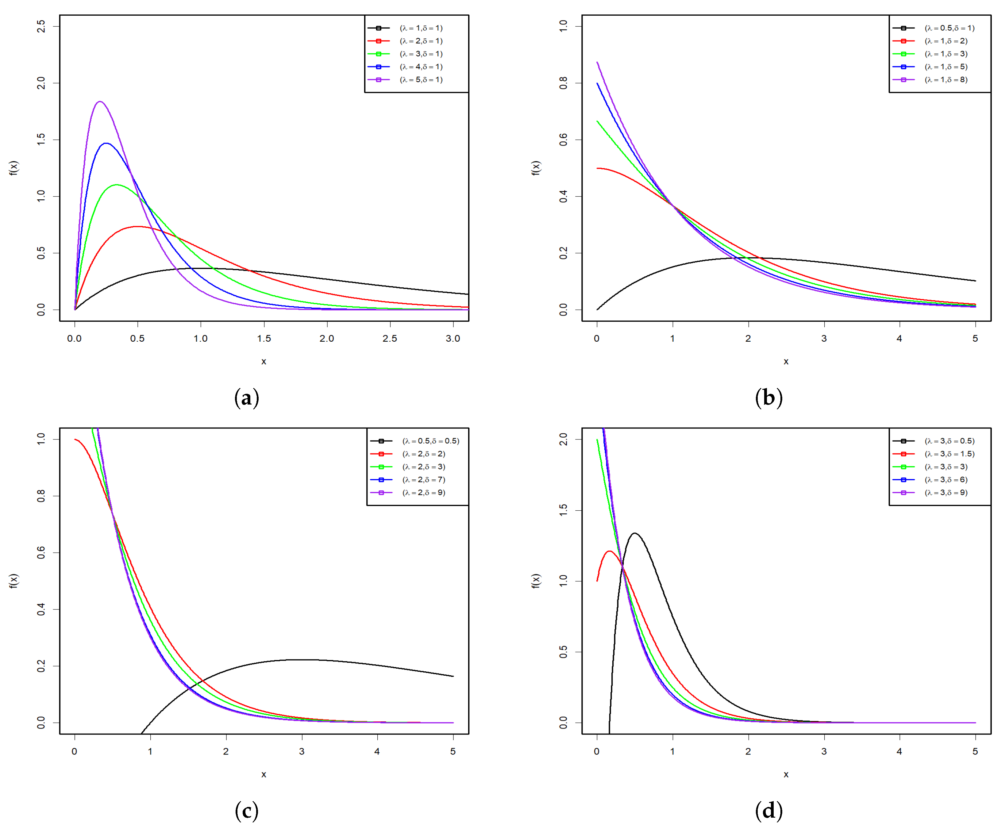
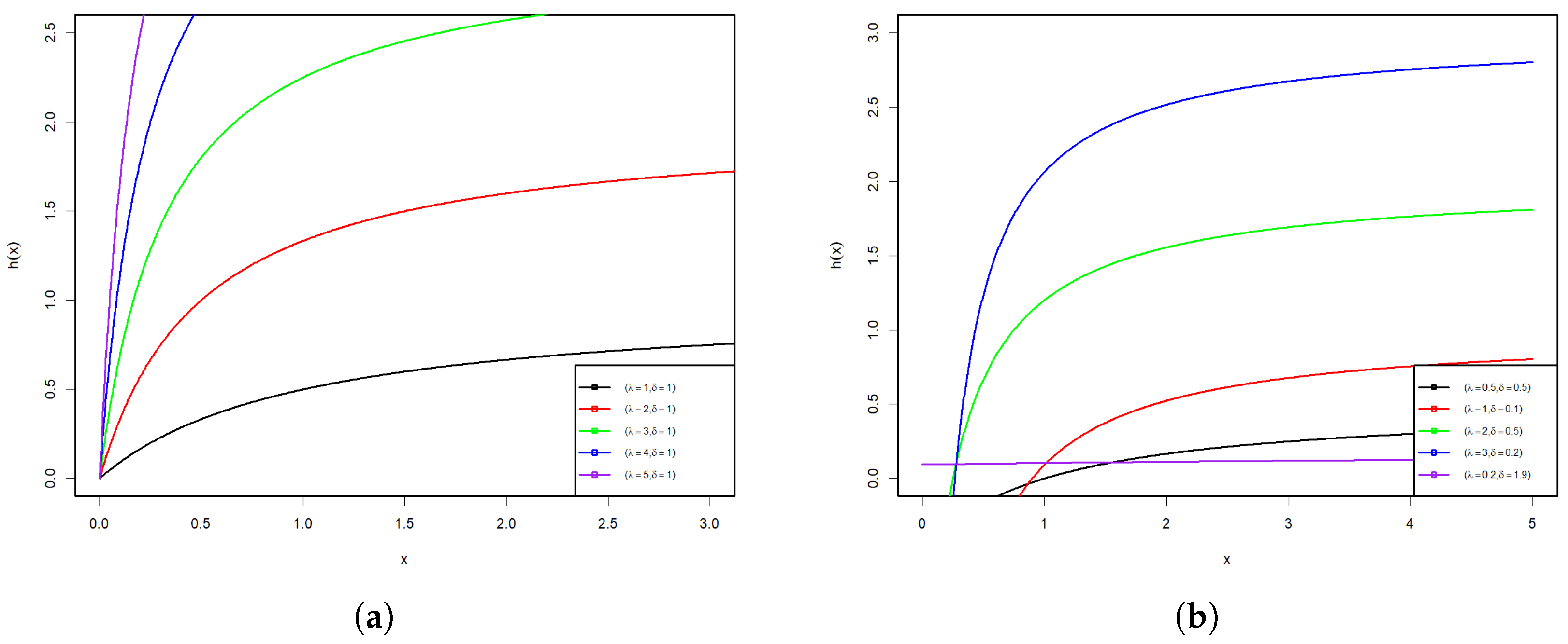
Figure 1 and Figure 2 display some graphs of the PDF and HRF of the PsL distribution for various parameter values. Figure 1a–d shows that the PDF of the PsL distribution has many shapes, such as right-skew, inverted bathtub, and inverse-J shaped, along with different Kurtosis. Conversely, Figure 2a,b reveals that the HRF of PsL distribution is increasing and constant.
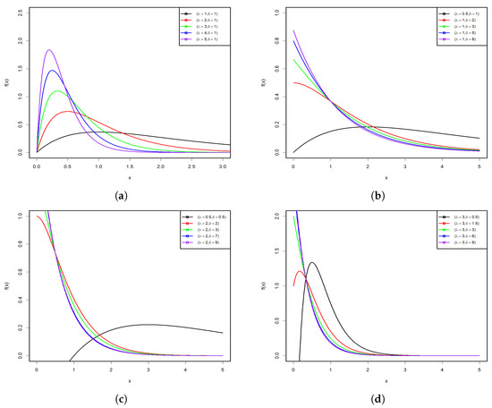
Figure 1.
PDF plots of the PsL distribution for various parameter values.
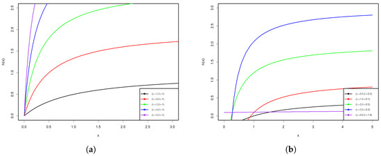
Figure 2.
HRF plots of the PsL distribution for various parameter values.
3. Acceptance Sampling Plans
Assuming that the lifespan of the product conforms to the PsL distribution characterized by two parameters—which are denoted as and , as described in Equation (2)—and that the declared median, denoted as M, of the units asserted by a manufacturer is , then our objective is to conclude whether the proposed batch should be accepted or rejected based on the condition that the actual median lifespan of the units exceeds the predetermined threshold . A common procedure in life testing involves concluding the test at a predefined time t and recording the count of failures. To determine the median lifetimes, the experiment is carried out throughout units. The ASP has been extensively investigated in various studies like [8,9,15,41,42,43,44]. Ref. [43] describes the concept of accepting the offered batch based on evidence that , with a probability of at least (consumer’s risk), by taking into account the ASP. The process to determine this is as follows: Obtain a random sample comprising n units from the proposed batch and perform an experiment throughout t units of time. If, through the experiment, fewer units (referred to as the acceptance number)—denoted by c—fail, then the entire lot is accepted; otherwise, the lot is rejected. As per the suggested ASP, the accepting probability of a batch is determined by considering batches of sufficient size to facilitate the application of the binomial distribution. This probability is expressed as
where , which is defined by (2). The function denotes the operational characteristic of the sampling plan, which represents the acceptance probability of the lot relative to the failure probability. Moreover, utilizing the formula , can be expressed accordingly:
The challenge is identifying the lowest positive integer n given specific values of and . Consequently, the function of operating characteristics can be reformulated as follows:
where the is given by (6). The n smallest values that meet the inequality (7) and their corresponding operational characteristic probabilities are determined and presented in Table 1, Table 2, Table 3, Table 4, Table 5 and Table 6 for the assumed parameters as follows:

Table 1.
Sampling plan for the PsL distribution with and .

Table 2.
Sampling plan for the PsL distribution with and .

Table 3.
Sampling plan for the PsL distribution with and .

Table 4.
Sampling plan for the PsL distribution with and .

Table 5.
Sampling plan for the PsL distribution with and .

Table 6.
Sampling plan for the PsL distribution with and .
- Consumer risk assumptions: is taken as 0.25, 0.5, and 0.95.
- Acceptance numbers for each proposed lot: c is set as 0, 2, 8, and 10.
- The factor median lifetime, denoted as a, is assumed as 0.25, 0.45, 0.60, 0.80, and 1. If a = 1, then for all values of and .
- Six parameter cases for the PsL distribution were considered , , , , and (0.20.
From the results presented in Table 1, Table 2, Table 3, Table 4, Table 5 and Table 6, we observed the following findings:
- Concerning the parameters of the ASP, as both and c increase, the necessary sample sizes n increases and the corresponding decreases.
- When the value of a increases, the sample size n decreases and increases.
- In all tables, for , we had since ; thus, all outcomes for any parameter vector were identical.
4. Classical Inference Methods
Here, we estimate the PsL distribution parameters using various non-Bayesian methods, including ML, LS, AD, MPS, and CVM estimation methods.
Assuming that , then the log-likelihood (L) function for the PsL distribution is given by
Taking the logarithm of the L function and simplifying gives
For and , the partial derivatives of the ℓ are given as follows
and
To find the MLEs of the PsL distribution, we had to find the values of and that maximize the ℓ function in (9), when (10) and (11) equate to zero. This can be conducted using numerical optimization techniques like the Newton-Raphson method in the R studio programming language.
Subject to certain regularity conditions, the MLEs () exhibited an approximate bi-variate normal distribution with mean (), which are denoted as , as well as a covariance matrix, which is denoted as , where
The asymptotic variances for the and were determined by the diagonal elements of matrix . Subsequently, the confidence interval for both and can be established using a normal approximation in the following equations: and .
Assume that the are the order-random observations associated with a random sample of size k drawn from the PsL distribution.
The LS estimation method can be used to estimate the parameters and of the PsL distribution based on a set of observed data by minimizing the LS function for the PsL distribution concerning and , which is defined in the following equations:
The AD method is a statistical method used for goodness-of-fit testing and the estimation of parameters in probability distributions. The AD method was introduced by [45]. The AD estimators of and for the PsL distribution were calculated by minimizing the AD function, which is given as follows:
The MPS estimator is a non-parametric method for estimating the unknown parameters of a probability distribution based on the product of spacings between ordered sample values (Ferguson & Klass, 1972) [46]. The MPS estimators of and for the PsL distribution were determined by minimizing the
where is the uniform spacings from the PsL distribution, and . Then, we have
The CVM method of estimation for the PsL distribution involves finding the parameters and that minimize the CVM function , which measures the discrepancy between the empirical distribution function of a sample and the theoretical function of the PsL distribution. The CVM estimators of and were obtained by minimizing
5. Bayesian Estimation (BE) Methods
BE is a statistical method that allows for the inference of unknown parameters by combining prior knowledge and observed data. In BE, a prior distribution is specified for the parameter(s) of interest, which represents the beliefs or assumptions about the parameter(s) before observing any data. Then, the observed data are used to update the prior distribution to a posterior distribution using Bayes’ theorem.
Here, we suppose that parameter has a gamma prior distribution and has a shifted gamma prior distribution due to [47,48]. Therefore, we have
and the joint prior distribution of the is obtained as follows:
The corresponding joint posterior of is given as follows:
so
where , and are called hyper-parameters, while K is called the normalizing constant.
In the context of this study, an exploration of three diverse loss functions was carried out, where, among these, the SE loss function was widely utilized, which is given by
where the is an estimator of the . Moreover, employing the SE loss function within the Bayesian framework results in an equal penalty for both overestimation and underestimation. A solution for such challenges is to utilize the LINEX and GE loss functions.
The definition of the LINEX loss function is as follows:
The GE loss function is defined as follows:
Now, through using the SE loss function, the BEs of the are given by
In using the LINEX loss function, the BEs of the are given by
and the BEs of the , through using the GE loss function, are obtained by
Since the above Equations (24)–(26) are hard to calculate analytically, we used the MCMC to estimate the unknown parameters using the R program. Next, we employed the MCMC method to produce posterior samples and to determine appropriate BEs. The MCMC technique serves as a useful simulation method for calculating quantities of interest in the posterior and sampling from posterior distributions. Utilizing the MCMC method with the aforementioned three functions, one can determine the Bayesian estimates for through the subsequent steps:
and
where represents the burn-in period of the MCMC. The construction of credible intervals (CI) for and can be achieved by following the algorithm detailed in [49]. Therefore, the credible interval for is .
6. Simulation Study
In this section, we evaluate the performance of non-Bayesian and Bayesian estimators for the parameters of the PsL distribution. The Bayesian estimation was conducted using the SE, GE, and LINEX loss functions, as discussed earlier. The simulation considered various scenarios with different values for , and . In the LINEX loss function, we examine two values of , which were and . Similarly, under the GE loss function, we considered and . The random sample of sizes and 200 were taken. The assessment of the estimator’s effectiveness was based on the mean squared error (MSE), average interval length (AIL), root mean squared error (RMSE), bias, confidence interval (CI), and coverage probability (CP). The results of the non-Bayes estimates are recorded in Table 7, Table 8, Table 9, Table 10, while the Bayes results are shown in Table 11, Table 12, Table 13, Table 14.

Table 7.
The MSE, RMSE, bias, CI, AIL, and CP for the PsL parameters when using non-Bayesian methods, with and .

Table 8.
The MSE, RMSE, bias, CI, AIL, and CP for the PsL parameters when using non-Bayesian methods, with and .

Table 9.
The MSE, RMSE, bias, CI, AIL, and CP for the PsL parameters when using non-Bayesian methods, with and .

Table 10.
The MSE, RMSE, bias, CI, AIL, and CP for the PsL parameters when using non-Bayesian methods, with and .

Table 11.
The MSE, RMSE, bias, CI, AIL, and CP for the PsL parameters when using Bayesian methods, with and .

Table 12.
The MSE, RMSE, bias, CI, AIL, and CP for the PsL parameters when using Bayesian methods, with and .

Table 13.
The MSE, RMSE, bias, CI, AIL, and CP for the PsL parameters when using Bayesian methods, with and .

Table 14.
The MSE, RMSE, bias, CI, AIL, and CP for the PsL parameters when using Bayesian methods, with and .
The tabulated values revealed the below observations.
Each of the estimators demonstrated consistent behavior, where the MSE, RMSE, bias, and AIL decreased with an increase in the sample size n, while the CP increased as the sample size n increased.
In all examined scenarios, both classical and Bayesian, as well as the MSE, RMSE, bias, and AIL of the estimator(s) for and , the metrics rose with higher values of the and parameters, while keeping n fixed. However, when n is constant, no consistent pattern was evident in the CP.
In classical estimation, ADE demonstrates superior efficiency compared to other estimators, followed by CVME and LSE.
For Bayes estimates, selecting is a preferable value for determining the BEs for both the GE and LINEX loss functions. The BEs using the LINEX loss function demonstrated greater efficiency compared to those using the SE and GE loss functions. Generally, the MSE follows the order: MSE (LINEX) ≤ MSE (GE) ≤ MSE (SE).
7. Real Data
As shown in this section, eight methods were employed to estimate the PsL parameters. One method utilizes Bayesian estimation (BE) under the square error loss function, whereas the remaining methods are non-Bayesian. Goodness-of-fit statistics, such as the Anderson–Darling (A*), Cramer–Von Mises (W*), and Kolmogorov–Smirnov (K-S) tests, along with the p-value related to the Kolmogorov–Smirnov (K-S) test, were used to compare the performance of the estimation methods.
The dataset below presents the failure times (in minutes) for a sample of 15 electronic components subjected to an accelerated life test, as documented in Lawless (2003, p. 204) [50]: (1.4, 5.1, 6.3, 10.8, 12.1, 18.5, 19.7, 22.2, 23.0, 30.6, 37.3, 46.3, 53.9, 59.8, 66.2).
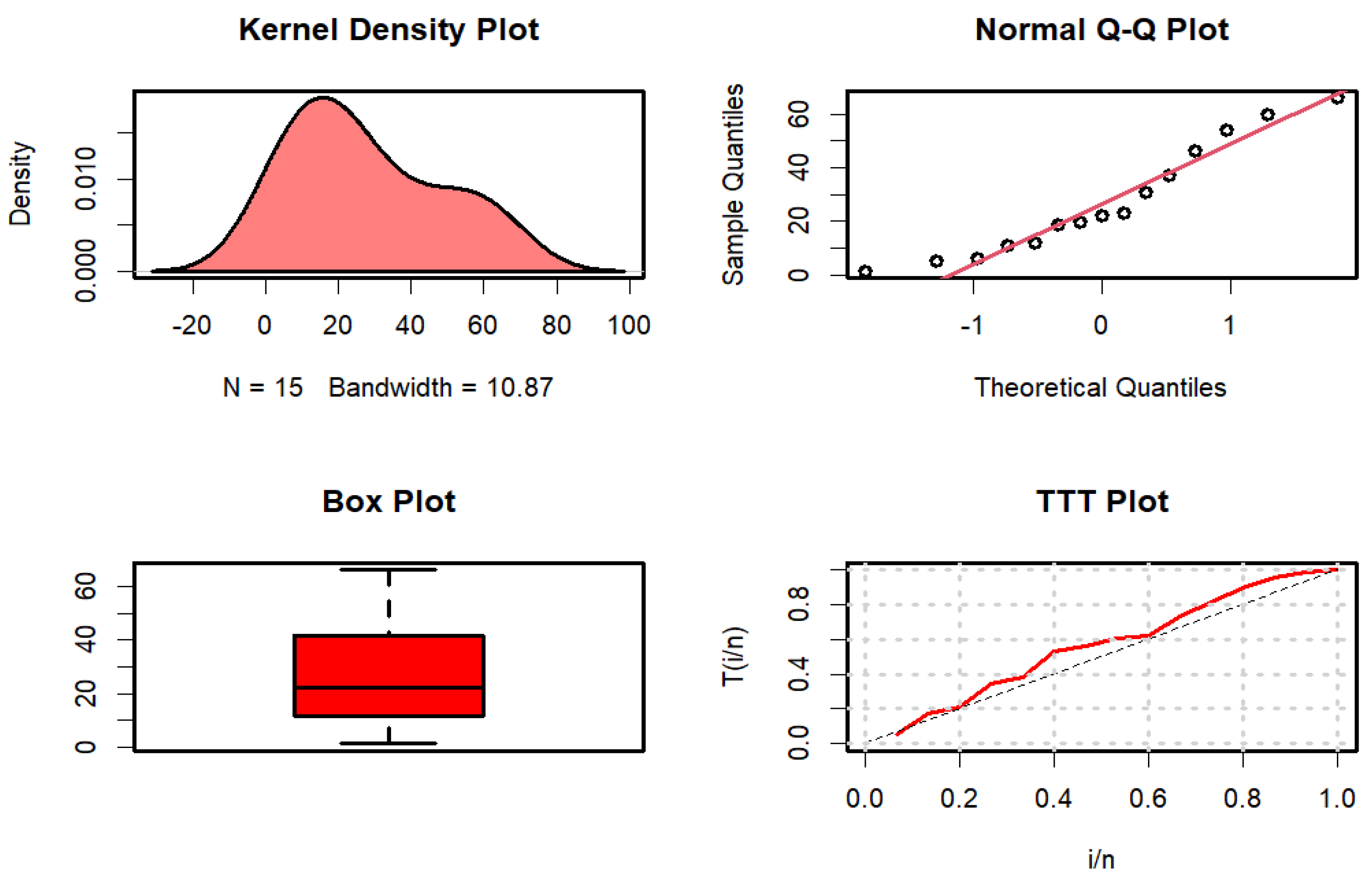
Figure 3 displays the kernel density, quantile-quantile (Q-Q), box, and time-to-target (TTT) plots.
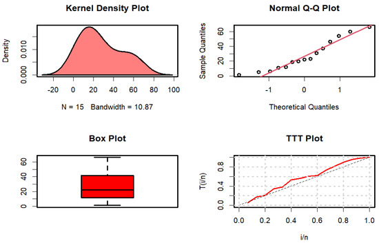
Figure 3.
Kernel density, Q-Q, box, and TTT plots for failure time data.
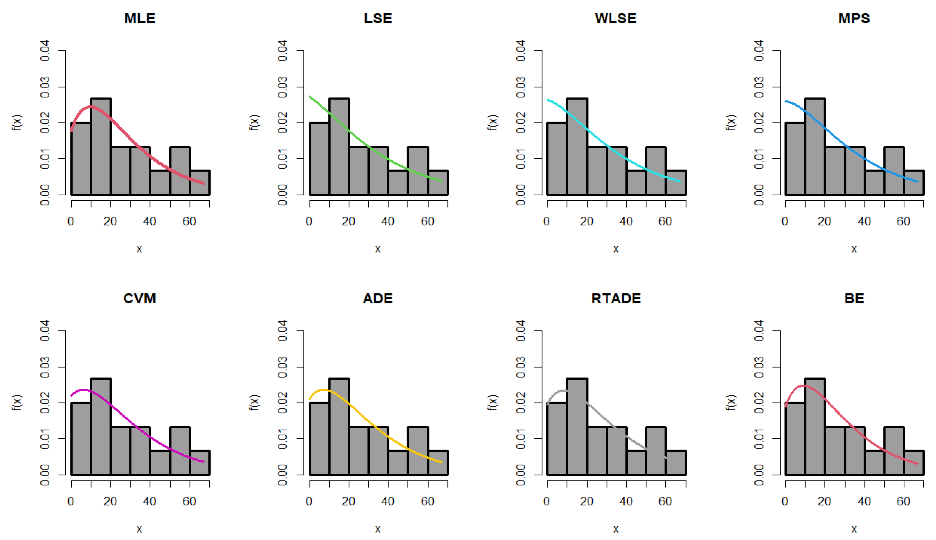
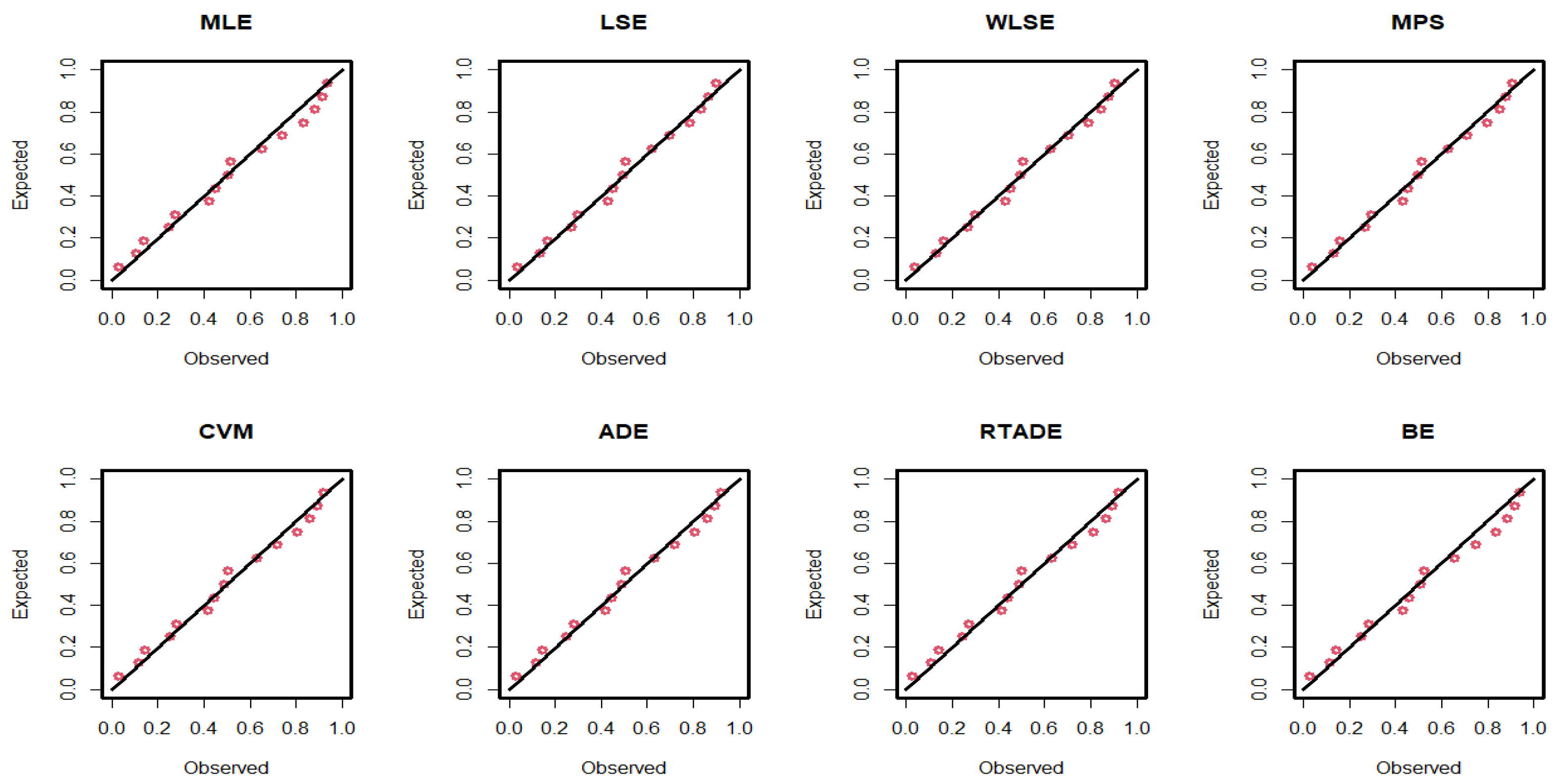
The estimated parameter values, along with the standard errors (SEs) for the MLEs, MPS, LSEs, WLSEs, CVMEs, ADEs, RTADEs, and BEs for the PsL distribution, are presented in Table 15. It is shown that the K-S statistic value for the MLE was smaller than those for the other methods, and the p-value of the K-S test for the MLE was greater than those for the others. Therefore, the MLE method outperformed the others, as demonstrated in Figure 4 and Figure 5. The following assumptions were used to determine the probability of the operational characteristics and the minimum values of n in the failure time data; for more details, refer to Table 16.

Table 15.
Estimated values with corresponding SEs (in brackets) for various estimator methods.
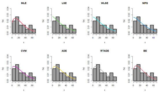
Figure 4.
Fitted PDF of the PsL distribution for the failure time data.
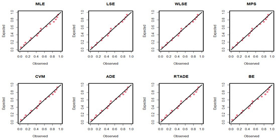
Figure 5.
P-P plots of the PsL distribution for the failure time data.

Table 16.
The ASP for the PsL distribution with parameters where and .
8. Conclusions
In this study, an ASP was developed using the PsL distribution, where the life test ended at the median lifetime of the PsL distribution. Various truncation periods, along with different characteristics of the PsL distribution and levels of consumer risk, were considered to determine the necessary sample size. Moreover, it was ensured that the acceptance probability at the attained sample sizes remained below or equal to the complement of the consumer’s risk.
The other aspect of this study involves investigating the estimation of parameters for the PsL distribution by employing the two types of estimators, i.e., classical methods and Bayesian methods, with symmetric and asymmetric loss functions. The BEs were derived using the SE, GE, and LINEX loss functions while utilizing appropriate priors on the parameters. Due to the unavailability of closed-form solutions for Bayes estimates under these loss functions, this study employed the MCMC technique. Through extensive simulation studies, we evaluated the performance of the considered methods of estimation under the specified loss functions. Finally, we demonstrated the potential applicability of the PsL distribution by applying it to real-world data, thus providing a practical context for assessing the effectiveness of different estimation methods.
Author Contributions
Conceptualization, F.Y.E.; Methodology, F.Y.E., C.D.S. and O.A.A.; Software, A.H.T.; Validation, C.D.S. and A.H.T.; Formal analysis, F.Y.E. and A.H.T.; Investigation, C.D.S. and A.H.T.; Resources, O.A.A.; Writing—original draft, F.Y.E.; Writing—review & editing, C.D.S. and A.H.T.; Visualization, O.A.A. All authors have read and agreed to the published version of the manuscript.
Funding
This research received no external funding.
Data Availability Statement
Data are contained within the article.
Conflicts of Interest
The authors declare no conflicts of interest.
References
- Irshad, M.R.; Chesneau, C.; D’Cruz, V.; Maya, R. Discrete pseudo Lindley distribution: Properties, estimation and application on INAR (1) process. Math. Comput. Appl. 2021, 26, 76. [Google Scholar] [CrossRef]
- Zeghdoudi, H.; Nedjar, S. On Poisson pseudo Lindley distribution: Properties and applications. J. Probab. Stat. Sci. 2017, 15, 19–28. [Google Scholar]
- Diallo, M.; Ngom, M.; Fall, A.M.; Lo, G.S. On the Kumaraswamy Pseudo-Lindley distribution: Statistical properties, extremal characterization and record values. Afr. Stat. 2022, 17, 3259–3291. [Google Scholar] [CrossRef]
- Gupta, S.S.; Gupta, S.S. Gamma distribution in acceptance sampling based on life tests. J. Am. Stat. Assoc. 1961, 56, 942–970. [Google Scholar] [CrossRef]
- Balakrishnan, N.; Leiva, V.; Lopez, J. Acceptance sampling plans from truncated life tests based on the generalized Birnbaum–Saunders distribution. Commun. Stat. Comput. 2007, 36, 643–656. [Google Scholar] [CrossRef]
- Schilling, E.G.; Neubauer, D.V. Acceptance Sampling in Quality Control; Chapman and Hall/CRC: Boca Raton, FL, USA, 2009. [Google Scholar]
- Aslam, M.; Kundu, D.; Ahmad, M. Time truncated acceptance sampling plans for generalized exponential distribution. J. Appl. Stat. 2010, 37, 555–566. [Google Scholar] [CrossRef]
- Nassr, S.G.; Hassan, A.S.; Alsultan, R.; El-Saeed, A.R. Acceptance sampling plans for the three-parameter inverted Topp–Leone model. Math. Biosci. Eng. 2022, 19, 13628–13659. [Google Scholar] [CrossRef] [PubMed]
- Chinedu, E.Q.; Chukwudum, Q.C.; Alsadat, N.; Obulezi, O.J.; Almetwally, E.M.; Tolba, A.H. New lifetime distribution with applications to single acceptance sampling plan and scenarios of increasing hazard rates. Symmetry 2023, 15, 1881. [Google Scholar] [CrossRef]
- Shahbaz, S.H.; Khan, K.; Shahbaz, M.Q. Acceptance sampling plans for finite and infinite lot size under power Lindley distribution. Symmetry 2018, 10, 496. [Google Scholar] [CrossRef]
- Al-Omari, A.I.; Al-Nasser, A. A two-parameter quasi Lindley distribution in acceptance sampling plans from truncated life tests. Pak. J. Stat. Oper. Res. 2019, XV, 39–47. [Google Scholar]
- Dhanunjaya, S.; Akhtar, P.M.; Venkatesulu, G. Continuous Acceptance Sampling plans for Truncated Lindley Distribution Based on CUSUM Schemes. Int. J. Math. Trends Technol.-IJMTT 2019, 65, 117–129. [Google Scholar] [CrossRef]
- Saha, M.; Tripathi, H.; Dey, S.; Maiti, S.S. Acceptance sampling inspection plan for the Lindley and power Lindley distributed quality characteristics. Int. J. Syst. Assur. Eng. Manag. 2021, 12, 1410–1419. [Google Scholar] [CrossRef]
- Wu, C.W.; Shu, M.H.; Wu, N.Y. Acceptance sampling schemes for two-parameter Lindley lifetime products under a truncated life test. Qual. Technol. Quant. Manag. 2021, 18, 382–395. [Google Scholar] [CrossRef]
- Tolba, A.H.; Onyekwere, C.K.; El-Saeed, A.R.; Alsadat, N.; Alohali, H.; Obulezi, O.J. A New Distribution for Modeling Data with Increasing Hazard Rate: A Case of COVID-19 Pandemic and Vinyl Chloride Data. Sustainability 2023, 15, 12782. [Google Scholar] [CrossRef]
- Tashkandy, Y.; Emam, W.; Ali, M.M.; Yousof, H.M.; Ahmed, B. Quality control testing with experimental practical illustrations under the modified Lindley distribution using single, double, and multiple acceptance sampling plans. Mathematics 2023, 11, 2184. [Google Scholar] [CrossRef]
- Ghitany, M.E.; Atieh, B.; Nadarajah, S. Lindley distribution and its application. Math. Comput. Simul. 2008, 78, 493–506. [Google Scholar] [CrossRef]
- Ghitany, M.; Alqallaf, F.; Al-Mutairi, D.K.; Husain, H. A two-parameter weighted Lindley distribution and its applications to survival data. Math. Comput. Simul. 2011, 81, 1190–1201. [Google Scholar] [CrossRef]
- Ghitany, M.; Al-Mutairi, D.K.; Balakrishnan, N.; Al-Enezi, L. Power Lindley distribution and associated inference. Comput. Stat. Data Anal. 2013, 64, 20–33. [Google Scholar] [CrossRef]
- Singh, B. Parameter Estimation of Power Lindly Distribution Under Hybrid Censoring. J. Stat. Appl. Probab. Lett. 2015, 1, 95–104. [Google Scholar] [CrossRef]
- Sharma, V.K.; Singh, S.K.; Singh, U. Classical and Bayesian methods of estimation for power Lindley distribution with application to waiting time data. Commun. Stat. Appl. Methods 2017, 24, 193–209. [Google Scholar] [CrossRef]
- Pak, A.; Ghitany, M.; Mahmoudi, M.R. Bayesian inference on power Lindley distribution based on different loss functions. Braz. Stat. Assoc. 2019, 33, 894–914. [Google Scholar] [CrossRef]
- Ghitany, M.; Al-Mutairi, D.K.; Aboukhamseen, S. Estimation of the reliability of a stress-strength system from power Lindley distributions. Commun. Stat.-Simul. Comput. 2015, 44, 118–136. [Google Scholar] [CrossRef]
- Joukar, A.; Ramezani, M.; MirMostafaee, S. Estimation of P (X > Y) for the power Lindley distribution based on progressively type II right censored samples. J. Stat. Comput. Simul. 2020, 90, 355–389. [Google Scholar] [CrossRef]
- Nadarajah, S.; Bakouch, H.S.; Tahmasbi, R. A generalized Lindley distribution. Sankhya B 2011, 73, 331–359. [Google Scholar] [CrossRef]
- Singh, S.K.; Singh, U.; Sharma, V.K. Expected total test time and Bayesian estimation for generalized Lindley distribution under progressively Type-II censored sample where removals follow the beta-binomial probability law. Appl. Math. Comput. 2013, 222, 402–419. [Google Scholar] [CrossRef]
- Singh, S.K.; Singh, U.; Sharma, V.K. Bayesian estimation and prediction for the generalized Lindley distribution under asymmetric loss function. Hacet. J. Math. Stat. 2014, 43, 661–678. [Google Scholar]
- Asgharzadeh, A.; Bakouch, H.S.; Nadarajah, S.; Sharafi, F. A new weighted Lindley distribution with application. Braz. J. Probab. Stat. 2016, 30, 1–27. [Google Scholar] [CrossRef]
- Rama, S. A quasi Lindley distribution. Afr. J. Math. Comput. Sci. Res. 2013, 6, 64–71. [Google Scholar]
- Shanker, R.; Sharma, S.; Shanker, U.; Shanker, R. Janardan distribution and its application to waiting times data. Indian J. Appl. Res. 2013, 3, 500–502. [Google Scholar] [CrossRef]
- Tolba, A.H.; Almetwally, E.M. Bayesian and Non-Bayesian Inference for The Generalized Power Akshaya Distribution with Application in Medical. Comput. J. Math. Stat. Sci. 2023, 2, 31–51. [Google Scholar]
- Kaminskiy, M.P.; Krivtsov, V.V. A simple procedure for Bayesian estimation of the Weibull distribution. IEEE Trans. Reliab. 2005, 54, 612–616. [Google Scholar] [CrossRef]
- Tolba, A.H. Bayesian and non-Bayesian estimation methods for simulating the parameter of the Akshaya distribution. Comput. J. Math. Stat. Sci. 2022, 1, 13–25. [Google Scholar] [CrossRef]
- Ahmad, H.H.; Almetwally, E. Marshall-Olkin generalized Pareto distribution: Bayesian and non Bayesian estimation. Pak. J. Stat. Oper. Res. 2020, 16(1), 21–33. [Google Scholar] [CrossRef]
- Gupta, P.K.; Singh, A.K. Classical and Bayesian estimation of Weibull distribution in presence of outliers. Cogent Math. 2017, 4, 1300975. [Google Scholar] [CrossRef]
- Singh, S.K.; Singh, U.; Yadav, A.S. Parameter estimation in Marshall-Olkin exponential distribution under Type-I hybrid censoring scheme. J. Stat. Appl. Probab. 2014, 3, 117. [Google Scholar] [CrossRef]
- Won, D.Y.; Lim, J.H.; Sim, H.S.; Sung, S.i.; Lim, H.; Kim, Y.S. A review on the analysis of life data based on Bayesian method: 2000∼2016. J. Appl. Reliab. 2017, 17, 213–223. [Google Scholar]
- Zeghdoudi, H.; Nedjar, S. A pseudo Lindley distribution and its application. Afr. Stat. 2016, 11, 923–932. [Google Scholar] [CrossRef]
- Nedjar, S.; Zeghdoudi, H. On Pseudo Lindley distribution: Properties and applications. New Trends Math. Sci. 2017, 5, 59–65. [Google Scholar] [CrossRef]
- Lo, G.S.; Kpanzou, T.A.; Haidara, M.C. Statistical tests for the Pseudo-Lindley distribution and applications. Afr. Stat. 2019, 14, 2127–2139. [Google Scholar]
- Alsadat, N.; Hassan, A.S.; Elgarhy, M.; Chesneau, C.; El-Saeed, A.R. Sampling Plan for the Kavya–Manoharan Generalized Inverted Kumaraswamy Distribution with Statistical Inference and Applications. Axioms 2023, 12, 739. [Google Scholar] [CrossRef]
- Abushal, T.A.; Hassan, A.S.; El-Saeed, A.R.; Nassr, S.G. Power Inverted Topp–Leone Distribution in Acceptance Sampling Plans. Comput. Mater. Contin. 2021, 67, 991–1011. [Google Scholar] [CrossRef]
- Singh, S.; Tripathi, Y.M. Acceptance sampling plans for inverse Weibull distribution based on truncated life test. Life Cycle Reliab. Saf. Eng. 2017, 6, 169–178. [Google Scholar] [CrossRef]
- Maya, R.; Irshad, M.R.; Ahammed, M.; Chesneau, C. The Harris Extended Bilal Distribution with Applications in Hydrology and Quality Control. Appl. Math. 2023, 3, 221–242. [Google Scholar] [CrossRef]
- Anderson, T.W.; Darling, D.A. Asymptotic theory of certain “goodness of fit” criteria based on stochastic processes. Ann. Math. Stat. 1952, 23, 193–212. [Google Scholar] [CrossRef]
- Ferguson, T.S.; Klass, M.J. A representation of independent increment processes without Gaussian components. Ann. Math. Stat. 1972, 43, 1634–1643. [Google Scholar] [CrossRef]
- Kim, S.; Lee, J.Y.; Sung, D.K. A shifted gamma distribution model for long-range dependent internet traffic. IEEE Commun. Lett. 2003, 7, 124–126. [Google Scholar]
- Wu, N.; Geistefeldt, J. Modeling travel time for reliability analysis in a freeway network. In Proceedings of the Conference: TRB 2016, Washington, DC, USA, 10–14 January 2016. [Google Scholar]
- Chen, M.H.; Shao, Q.M. Monte Carlo estimation of Bayesian credible and HPD intervals. J. Comput. Graph. Stat. 1999, 8, 69–92. [Google Scholar] [CrossRef]
- Lawless, J.F. Statistical Models and Methods for Lifetime Data; John Wiley & Sons: Hoboken, NJ, USA, 2011. [Google Scholar]
Disclaimer/Publisher’s Note: The statements, opinions and data contained in all publications are solely those of the individual author(s) and contributor(s) and not of MDPI and/or the editor(s). MDPI and/or the editor(s) disclaim responsibility for any injury to people or property resulting from any ideas, methods, instructions or products referred to in the content. |
© 2024 by the authors. Licensee MDPI, Basel, Switzerland. This article is an open access article distributed under the terms and conditions of the Creative Commons Attribution (CC BY) license (https://creativecommons.org/licenses/by/4.0/).

