Small Area Estimation under Poisson–Dirichlet Process Mixture Models

Abstract

In this paper, we propose an improved Nested Error Regression model in which the random effects for each area are given a prior distribution using the Poisson–Dirichlet Process. Based on this model, we mainly investigate the construction of the parameter estimation using the Empirical Bayesian(EB) estimation method, and we adopt various methods such as the Maximum Likelihood Estimation(MLE) method and the Markov chain Monte Carlo algorithm to solve the model parameter estimation jointly. The viability of the model is verified using numerical simulation, and the proposed model is applied to an actual small area estimation problem. Compared to the conventional normal random effects linear model, the proposed model is more accurate for the estimation of complex real-world application data, which makes it suitable for a broader range of application contexts.

1. Introduction

The study of small area estimation has received more and more attention due to the increasing demand for reliable estimates in governmental departments, enterprises, agriculture, commerce, and socioeconomic fields. The issue of how to improve the estimation accuracy and obtain reliable estimates of subpopulation parameters is known as small area estimation. The term “small area” usually refers to a small geographic area, such as a county, city, state, or a small population group that is crossclassified by demographic characteristics, such as a certain age, gender, or ethnic group. Since a majority of sample surveys are designed to estimate certain parameters for the overall population, there are no particular requirements for sample sizes for subgroups, which can lead to the possibility that the parameter estimates for subgroups may not be as accurate as desired. Furthermore, if the sample size of a survey is determined to achieve a specified level of accuracy on a large scale, there may not be enough resources to conduct a second survey aimed at achieving a similar level of accuracy on a smaller scale.

The application of indirect estimation, in particular model-based estimation for small areas, to address this issue has been widely accepted. Recognizing the commonality or similarity of several small areas in certain aspects, we can construct reliable small area estimates with the help of well-defined models, thus borrowing relevant auxiliary information from other variables in the area, from neighboring small areas, or even from other sources, such as population census data. This concept has also greatly contributed to the development of the small area estimation problem, and various models and methods have been proposed to estimate small area parameters by borrowing auxiliary information. For example, one can check the publications of Rao [1] and Pfeffermann [2] for understanding and reviewing. Rao and Molina [3] give a detailed and previous description of the models and methods for small area estimation.

Fay and Herriot [4] were the first to propose an area level model, the Fay-Herriot model, to solve the problem of small area estimation of per capita income in the USA. Battese, Harter, and Fuller [5] were the first to adopt the unit level model, the Nested Error Regression Model, which combines agricultural survey data and satellite data, to estimate the average acreage of crops in twelve counties in the state of Iowa in the United States. With the growing demand for small area estimation, there has been a large amount of literature on extending these two base models to accommodate different data structures and requirements. For example, Serena et al. [6] provided two extensions of the Fay–Herriot model. The first one is a multivariate extension, which jointly models the survey estimates of two or more different but related demographic characteristics; the second extension is to build a functional measurement error model into the original Fay–Herriot model to consider the case of covariates with errors. Yang and Chen [7] improved the Nested Error Regression model by clustering small areas based on their centers to obtain a new model and estimate the model parameters based on the model.

The accuracy and precision of small area estimators depend on the validity of the model. In this context, we pay particular attention to an important underlying assumption of the model, namely the normality of random effects. The assumption of normality of random effects is not necessarily reasonable for no reason other than computational convenience. In particular, this assumption is difficult to detect in practice because it involves unobservable quantities. Therefore, it is necessary to investigate the flexible modeling of random effects. Datta et al. [8] considered the case where random effects do not exist and proposed a bootstrap method for hypothesis testing that allows us to determine the presence or absence of random effects in various regions of the model. This is because the use of random effects will increase the variability of the estimates when the actual data structure does not include random effects. Sugasawa and Kubokawa [9] also proposed a Nested Error Regression model that utilizes uncertain random effects and gave estimates of the corresponding model parameters. Ferrante and Pacei [10] considered the asymmetry of the data they examined and thus relaxed the normality assumption of the Fay–Herriot model by adopting a skewed distribution. They proposed a multivariate skewed small area model and applied the model to the business statistics of firms. Fabrizi and Trivisano [11] considered two extensions of the Fay–Herriot model where both extensions were for the assumptions of the random effects of the model, which were an exponential power distribution and a skewed power distribution. Chakraborty et al. [12] proposed a mixture model based on the Fay–Herriot model with random effects obeying a two-component normal form. Diallo and Rao [13] concerned themselves with the skewed distribution of the response variable and suggested replacing the assumption of normality for both random effects and errors with a skew normal distribution. Tsujino and Kubokawa [14] investigated a model in which the random effects remain normal but the errors obey a skew normal distribution, and they gave an expression for predicting the random effects.

In small area estimation, parametric models are usually used to build mixed models to achieve estimation. However, parametric models suffer from model mis-specification, which may produce unreliable small area estimations. The application of nonparametric and semiparametric models to achieve small area estimation has been partially considered in the literature. Opsomer et al. [15] used a p-spline approach applied to the nonparametric estimation of the regression component in a Nested Error Regression model linear model. Polettini [16] used a Dirichlet Process mixture model to implement the construction of random effects in the Fay–Herriot model.

To further extend the Nested Error Regression model, this paper proposes an improved Nested Error Regression model in which the default normality assumption for random effects is replaced by a nonparametric specification, i.e., using the Poisson–Dirichlet Process. In Nested Error Regression models, random effects are typically assumed to be normally distributed. This assumption simplifies the theoretical and computational analysis of the model. However, the normality assumption may not hold in certain cases, thus leading to inaccurate model estimates. To address this limitation, we propose the use of a nonparametric specification to replace the default normality assumption. Nonparametric methods do not rely on specific parameters or distributional forms; instead, they learn their structure or characteristics directly from the data. The Poisson–Dirichlet Process is proposed as a prior distribution for the random effects. This approach differs from the conventional assumption that the random effects in each area follow a fixed distribution. Instead, the model allows the distribution of these random effects to change adaptively based on the data. The Poisson–Dirichlet Process is a two-parameter generalization of the Dirichlet Process, where, in addition to the concentration parameter, an additional parameter called the discount parameter is also added. Similar to the Dirichlet Process, samples from the Poisson–Dirichlet Process correspond to discrete distributions that have the same support as its underlying distribution. The underlying distribution of the Poisson–Dirichlet Process is the Poisson–Dirichlet Distribution introduced by Pitman and Yor [17]. Due to its properties, we can apply it to the prior distribution of random effects, which has an unobservable variable. There are many studies related to the Dirichlet Process and the Poisson–Dirichlet Process in Bayesian nonparametrics. For example, Al-labadi et al. [18], by applying Bayesian estimation of the Dirichlet Process, proposed a novel methodology for computing varentropy and varextropy. Handa [19] studied a two-parameter Poisson–Dirichlet Process based on point process theory. Favaro et al. [20] developed a two-parameter Poisson–Dirichlet Process model for dealing with the problem of the predictive sampling of species or kinds. Performing exact Bayesian inference on nonparametric models is always challenging, because it is difficult to derive the posterior distribution. This drives us to use the Markov chain Monte Carlo (MCMC) algorithm [21] for approximate inference.

The paper is organized as follows: Section 2 reviews the classical Nested Error Regression model and the Poisson–Dirichlet Process. Section 3 describes the proposed model. In Section 4, the methods corresponding to the estimation of each parameter in the model and the algorithm flow are given. In Section 5 and Section 6, the feasibility of the model and the corresponding parameter estimation methods are investigated by applying them to simulated and real data. The article is briefly summarized in the last section.

2. Theoretical Background

2.1. Nested Error Regression Models

Battese, Harter, and Fuller [5] published a seminal paper that contributed to the popularization of model-based small area estimation in government statistics. Model-based small area estimation requires the use of appropriate regression models that relate area target variables to appropriate auxiliary variables obtained from other surveys and records administered by government agencies. These authors presented Nested Error Regression (NER) models, as well as a unit-level model that combines satellite data and farm-level survey observations to determine the average corn and soybean acreage in twelve counties in Iowa, USA.

Suppose that the population of interest U is partitioned into mutually m independent small areas $U_i$, where the total size is $N={\sum }_{i=1}^m{N}_i$, and the sample size is $n={\sum }_{i=1}^m{n}_i$. The sequence $\left(y_{i1},x_{i1}\right),\dots ,\left(y_{i{n}_i},x_{i{n}_i}\right)$ is the target variable and the corresponding covariate for the observation of the jth sample unit in the ith small area, where $i=1,2,\dots ,m$ is an indicator of the small areas. And $x_{ij}=\left(1,x_{i{j}_1},\dots ,x_{i{j}_{\left(p-1\right)}}\right)$ is a known p-dimensional vector of covariates. Battese et al. [5] proposed the following normal NER model:

$$y_{ij}=x_{ij}^{\prime }\beta +{\nu }_i+{\epsilon }_{ij}$$

(1)

where $\beta =\left({\beta }_0,\dots ,{\beta }_{p-1}\right)$ denotes the unknown p-dimensional vector of the regression coefficients, and ${\nu }_i$ and ${\epsilon }_{ij}$ denote the area-specific random effect and error, respectively, for the ith small area. It is assumed that the random effects ${\nu }_i$ and errors ${\epsilon }_{ij}$ follow normal distributions, ${\nu }_i\sim N\left(0,{\sigma }_{\nu }^2\right)$ and ${\epsilon }_{ij}\sim N\left(0,{\sigma }_{\epsilon }^2\right)$, and that the random effects ${\nu }_i$ and errors ${\epsilon }_{ij}$ are independent of each other. We frequently seek to obtain the estimated mean $\rho =\left({\rho }_1,\dots ,{\rho }_m\right)$ of the target variable for all small areas through the small area model, also known as the small area mean $\rho$. Assuming that the mean of the covariate $\overline{x}$ is available for each small area, the ith small area mean ${\rho }_i$ is defined by the following formula:

$${\rho }_i={\overline{x}}_i^{\prime }\beta +{\nu }_i$$

(2)

As shown below in the hierarchical Bayesian approach based on the model in Equation (1) for predicting ${\rho }_i$, this is accomplished by giving a prior distribution to the unknown model parameter $\psi =\left(\beta ,{\sigma }_{\nu }^2,{\sigma }_{\epsilon }^2\right)$.

The NER model can be described as follows:

• Define a conditional on $\rho =\left({\rho }_1,\dots ,{\rho }_m\right)$ and $\psi =\left(\beta ,{\sigma }_{\nu }^2,{\sigma }_{\epsilon }^2\right)$, as well as estimator $Y_i\sim N\left({\rho }_i,{\sigma }_{\nu }^2\right)$, for $i=1,2,\dots ,m$, independently;
• Define a conditional on $\psi =\left(\beta ,{\sigma }_{\nu }^2,{\sigma }_{\epsilon }^2\right)$ and small area means ${\rho }_i\sim N\left({\overline{x}}_i^{\prime }\beta ,{\sigma }_{\nu }^2\right)$, for $i=1,2,\dots ,m$, independently;
• The model parameters $\psi =\left(\beta ,{\sigma }_{\nu }^2,{\sigma }_{\epsilon }^2\right)$ are given a prior distribution with a density $\pi \left(\psi \right)$.

2.2. Poisson–Dirichlet Process

The Poisson–Dirichlet Process (PDP), also known as the Pitman–Yor Process, is a two-parameter extension of the Dirichlet Process. Similar to the Dirichlet Process, the Poisson–Dirichlet Process is a distribution placed on top of a distribution. The distribution underlying the Poisson–Dirichlet Process is the Poisson–Dirichlet Distribution. Assume that there exists a pair of parameters $\alpha$ and $\theta$ such that $0\le \alpha <1$ and $\theta >-\alpha$. Here, we name $\alpha$ as the discount parameter and $\theta$ as the concentration parameter. Let $V_1,V_2,\dots$ be a sequence of mutually independent random variables, and allow $V_k$ obey the following distribution: $V_k|\alpha ,\theta \sim Beta\left(1-\alpha ,\theta +k\alpha \right)$; define $\left(p_1,p_2,\dots \right)$ as follows:

$$p_1=V_1,p_k=V_k\prod _{i=1}^{k-1}\left(1-V_i\right)$$

(3)

Meanwhile, $\left(p_1,p_2,\dots \right)$ satisfies ${\sum }_{k=1}^{\infty }{p}_k=1$. If we arrange $\left(p_1,p_2,\dots \right)$ in descending order to obtain $p=\left({\tilde{p}}_1,{\tilde{p}}_2,\dots \right)$, then p is a Poisson-Dirichlet distribution, which is denoted as $p\sim PD\left(\alpha ,\theta \right)$. Having defined the Poisson–Dirichlet Distribution, we can formally define the Poisson–Dirichlet Process. Assume that the base distribution $H_0$ is a probability distribution on the measurable space $\left(\chi ,\mathcal{B}\right)$. Let $X_1,X_2,\dots$ be a sequence of independently and identically distributed random variables from the base distribution $H_0$, and assume that $p\sim PD\left(\alpha ,\theta \right)$; then, we define the random probability measure G on $\left(\chi ,\mathcal{B}\right)$ to be the Poisson–Dirichlet Process with parameters $\alpha$ and $\theta$ and base distribution $H_0$, which is given by the following:

$$G\left(x|\alpha ,\theta ,H_0\right)=\sum _{k=1}^{\infty }{p}_k{\delta }_{X_k}\left(x\right)$$

(4)

where ${\delta }_{X_k}\left(x\right)$ denotes the Dirac measure of degeneracy at point $X_k$: ${\delta }_{X_k}\left(x\right)=\left\{\begin{array}{cc}1,\hfill & x=X_k\hfill \\ 0,\hfill & otherwise\hfill \end{array}\right.$. This stick-breaking distribution G is also denoted as $G\sim PD\left(\alpha ,\theta ;H_0\right)$. The parameters $\alpha$ and $\theta$ determine the power law properties of the Poisson–Dirichlet Process. In practical modeling, the Poisson–Dirichlet Process is more appropriate than the Dirichlet Process, because it exhibits power law properties that can be captured in natural language, and $\alpha =0$ corresponds to the Dirichlet Process.

3. Small Area Model with PDP Random Effects

As in the NER model, in the proposed model, we assume that the observations $y_i=\left(y_{i1},y_{i2},\dots y_{i{n}_i}\right),i=1,2,\dots ,m$ are a set of data associated with independent and identically distributed random effects ${\nu }_i=\left({\nu }_{i1},\dots ,{\nu }_{i{n}_i}\right),i=1,2,\dots ,m$. We consider replacing the normal random effects prior distribution of the NER model with a Bayesian nonparametric prior; namely, we assume that ${\nu }_i=\left({\nu }_{i1},\dots ,{\nu }_{i{n}_i}\right),i=1,2,\dots ,m$ is independently and identically distributed, thus obeying an unknown probability measure $H_i,i=1,2,\dots ,m$. At this moment, the distribution of the random effects $H_i,i=1,2,\dots ,m$, as an unknown quantity, can be given a Bayesian nonparametric prior. In this section, by assuming $0\le \alpha <1$ and $\theta >-\alpha$, we introduce the Poisson–Dirichlet Process with parameters $\alpha$ and $\theta$ and a base distribution $H_0$ as a prior to assign the distributions $H_i,i=1,2,\dots ,m$ of the random effects to the model, and we obtain a unit-level small area model with PDP random effects:

$$y_{ij}=x_{ij}^{\prime }\beta +{\nu }_{ij}+{\epsilon }_{ij},j=1,2,\dots ,n_i,i=1,2,\dots ,m$$

(5)

where $x_{ij}$ is a known auxiliary variable in the p-dimension associated with the observation $y_{ij}$, $\beta$ is an unknown vector of regression coefficients in the p-dimension, ${\epsilon }_{ij}$ is a random variable with a mean of 0 and a variance of $Var\left({\epsilon }_{ij}\right)={\sigma }_{\epsilon }^2$, and ${\nu }_{ij}$ is a random effect with a magnitude reflecting the differences between units in different areas; ${\epsilon }_{ij}$ and ${\nu }_{ij}$ are mutual and independent, and they can be expressed as follows:

$${\epsilon }_{ij}\sim N\left(0,{\sigma }_{\epsilon }^2\right)j=1,2,\dots ,n_i;i=1,2,\dots ,m$$

(6)

$${\nu }_{i1},\dots ,{\nu }_{i{n}_i}|H_i\stackrel{iid}{\sim }{H}_{i}i=1,2,\dots ,m$$

(7)

$$H_i\sim PD\left(\alpha ,\theta ;H_0\right)$$

(8)

where $H_0$ is the base distribution, $\alpha$ is the discount parameter, and $\theta$ is the concentration parameter. Parameters $\alpha$ and $\theta$ determine not only the power law properties of the Poisson–Dirichlet Process, but also the probability that a new random effect ${\nu }_{ij}$ will be sampled if ${\nu }_{i1},\dots ,{\nu }_{ij-1}$ already exists and given $H_i$. In the proposed model, when a new random effect ${\nu }_{ij}$ is drawn, it either comes from one of the previous classes of ${\nu }_{i1},\dots ,{\nu }_{ij-1}$ or a new one from $H_i$. If ${\nu }_{ij}$ comes from one of the previous classes of ${\nu }_{i1},\dots ,{\nu }_{ij-1}$, its probability is positively related to the number of data points contained in this class. The larger the value of the parameter $\theta$, the greater the probability that ${\nu }_{ij}$ will be drawn from $H_i$ in a new class. For the random effects variable ${\nu }_i=\left({\nu }_{i1},\dots ,{\nu }_{i{n}_i}\right)$, let ${\nu }_{i1}^{*},\dots ,{\nu }_{i{K}_i}^{*}$ be the elements of ${\nu }_i=\left({\nu }_{i1},\dots ,{\nu }_{i{n}_i}\right)$ that are not identical to each other, let $K_i$ be the number of classes in ${\nu }_i=\left({\nu }_{i1},\dots ,{\nu }_{i{n}_i}\right)$, and let $m_{ik}$ be the number of elements in the kth class; then the sampling probability of ${\nu }_{ij}$ is as follows:

$$Pr\left({\nu }_{ij}={\nu }_{ik}^{*}|{\nu }_{i1},\dots ,{\nu }_{ij-1}\right)=\frac{m_{ik}-\alpha }{j-1+\theta },k=1,2,\dots ,K_i$$

(9)

$$Pr\left({\nu }_{ij}\notin \left\{{\nu }_{i1}^{*},\dots ,{\nu }_{i{K}_i}^{*}\right\}|{\nu }_{i1},\dots ,{\nu }_{ij-1}\right)=\frac{K_i\alpha +\theta }{j-1+\theta }$$

(10)

The hierarchical structure of our model can be represented as follows.

The NER model with PDP random effects:

• Define a conditional on $\nu =\left({\nu }_1,\dots ,{\nu }_m\right)$, ${\nu }_i=\left({\nu }_{i1},\dots ,{\nu }_{i{n}_i}\right)$, $\beta$, and ${\sigma }_{\epsilon }^2$; estimator $y_{ij}$ is given by $y_{ij}\sim N\left(x_{ij}^{\prime }\beta +{\nu }_{ij},{\sigma }_{\epsilon }^2\right)$, for $j=1,2,\dots ,n_i;i=1,2,\dots ,m$, independently;
• Define a conditional on $\alpha$, $\theta$, and $H_0$; the random effects $\nu$ are given by ${\nu }_{i1},\dots ,{\nu }_{i{n}_i}|H_i\stackrel{iid}{\sim }{H}_i$ and $H_i\sim PD\left(\alpha ,\theta ;H_0\right)$, for $j=1,2,\dots ,n_i;i=1,2,\dots ,m$, independently.

4. Estimation

In small area estimation, we aim to obtain good estimators of the small area mean ${\rho }_i$. Based on the proposed model, we mainly consider the estimation of the model parameters $\beta$, ${\sigma }_{\epsilon }^2$, $\alpha$, $\theta$, and $H_0$, and the conditional mean $\widetilde{{\rho }_i}\left(\beta ,{\sigma }_{\epsilon }^2,\alpha ,\theta ,H_0,y_{ij}\right)$ is given the data $y_{11},\dots ,y_{m{n}_m}$.

In the small area model with PDP random effects, for the ith small area, the random effect ${\nu }_{i1},\dots ,{\nu }_{i{n}_i}$ that comes from ${\nu }_{i1},\dots ,{\nu }_{i{n}_i}|H_i\sim H_i$, ${\nu }_{i1},\dots ,{\nu }_{i{n}_i}$ can be divided into mutually exclusive classes ${\nu }_{i1}^{*},\dots ,{\nu }_{i{K}_i}^{*}$, and we define $m_i=\left(m_{i1},\dots ,m_{i{K}_i}\right)$, where $m_{ij}$ denotes the number of contained elements in the jth class of the ith small area, and $K_i$ denotes the number of mutually exclusive classes in ${\nu }_{i1},\dots ,{\nu }_{i{n}_i}$. Assume that we assign data points $y_{i1},\dots ,y_{i{n}_i}$ according to the classes of ${\nu }_{i1},\dots ,{\nu }_{i{n}_i}$ to obtain $K_i$ groups: $\left(y_{i1}^1,\dots ,y_{i{m}_1}^1\right),\dots ,\left(y_{i1}^{K_i},\dots ,y_{i{m}_{K_i}}^{K_i}\right)$. The likelihood function of the model parameters $\beta$, ${\sigma }_{\epsilon }^2$, $\alpha$, $\theta$, and $H_0$ is

$$\begin{array}{cc}\hfill L\left(\beta ,{\sigma }_{\epsilon }^2,\alpha ,\theta ,H_0\right)& =E_{\nu }\left(\prod _{k=1}^{n_j}f\left(y_{ij}|{\nu }_{ij}\right)\right)=E_{\nu }\left(\prod _{j=1}^{m_{i1}}f\left(y_{ij}^1|{\nu }_{i1}^{*}\right)\dots \prod _{j=1}^{m_{i{K}_i}}f\left(y_{ij}^{K_i}|{\nu }_{i{K}_i}^{*}\right)\right)\hfill \\ \hfill & =E_{K,m}\left(\int \prod _{j=1}^{m_{i1}}f\left(y_{ij}^1|u\right)g_0\left(u\right)du\dots \int \prod _{j=1}^{m_{i{K}_i}}f\left(y_{ij}^{K_i}|u\right)g_0\left(u\right)du\right)\hfill \end{array}$$

(11)

where $E_x$ denotes the marginal expectation about x, f denotes the probability density function of normality, and $h_0$ denotes the density function of the base distribution $H_0$. This likelihood function is too complex to be maximized or numerical, so we consider applying empirical Bayesian estimation to solve the estimation of the model parameters.

In this section, we consider the application of empirical Bayesian nonparametric methods to study the estimation of the regression coefficients $\beta$ and the error variance ${\sigma }_{\epsilon }^2$ for the small area model with PDP random effects, as well as the estimation of the discounting parameter $\alpha$, the concentration parameter $\theta$, and the base distribution $H_0$ for the Poisson–Dirichlet Process when given the known data $y_{11},\dots y_{1n_1},\dots ,y_{m1},\dots ,y_{m{n}_m}$. We explain the algorithms used to derive these estimates in detail.

4.1. Proposed Approach

4.1.1. Estimation of Regression Coefficients and Error Variance

The first consideration we make is the estimation of the regression coefficients $\beta$ and the error variance ${\sigma }_{\epsilon }^2$ in the model. Assuming that the random effects ${\nu }_{ij}$ are known, by rewriting Equation (5) and defining $y_{ij}^{*}$ in the model, we obtain the following:

$$y_{ij}^{*}=y_{ij}-{\nu }_{ij}=x_{ij}^{\prime }\beta +{\epsilon }_{ij}j=1,2,\dots ,n_i,i=1,2,\dots ,m$$

(12)

We consider a matrix representation of the above equation such that $Y^{*}={\left(Y_1^{*},\dots ,Y_m^{*}\right)}^{\prime }$, and $X={\left(X_1,\dots ,X_m\right)}^{\prime }$ is a matrix with column rank $r\left(X\right)$ and error $\epsilon ={\left({\epsilon }_1,\dots ,{\epsilon }_m\right)}^{\prime }$. In this case, $Y_i^{*}={\left(y_{i1}^{*},\dots ,y_{i{n}_i}^{*}\right)}^{\prime }$, $X_i={\left(x_{i1},\dots ,x_{i{n}_i}\right)}^{\prime }$, and ${\epsilon }_i={\left({\epsilon }_{i1},\dots ,{\epsilon }_{i{n}_i}\right)}^{\prime }$; thus, we again obtain the following:

$$Y^{*}=X\beta +\epsilon$$

(13)

$$\epsilon \sim N\left(0,{\sigma }_{\epsilon }^2\right)$$

(14)

For the above linear regression model, we consider the idea of using the classical algorithm of parameter estimation for solving the regression model, that is, the least squares estimation algorithm, to obtain the estimates of the regression coefficients $\beta$ and the error variance ${\sigma }_{\epsilon }^2$.

For the regression coefficients $\beta$, the objective of least squares estimation is to find an estimate of the regression coefficients $\widehat{\beta }$ that minimizes the sum of the squared residuals of all sample observations $Q\left(\widehat{\beta }\right)=\sum {\left(Y_i^{*}-{\widehat{Y}}_i^{*}\right)}^2$. The sum of the squared residuals is easily obtained by derivation:

$$Q\left(\widehat{\beta }\right)=Y^{*\prime }{Y}^{*}-2{\widehat{\beta }}^{\prime }{X}^{\prime }{Y}^{*}+{\widehat{\beta }}^{\prime }{X}^{\prime }X\widehat{\beta }$$

(15)

By minimizing the sum of the squared residuals $Q\left(\widehat{\beta }\right)$ and assuming that ${\left(X^{\prime }X\right)}^{-1}$ exists, an estimate of the regression coefficient $\beta$ can be obtained as follows.

$$\widehat{\beta }={\left(X^{\prime }X\right)}^{-1}{X}^{\prime }{Y}^{*}$$

(16)

For the estimation of the error variance ${\sigma }_{\epsilon }^2$, we first consider that the error vector $\epsilon =Y^{*}-X\beta$ is an unobservable vector. Suppose we replace $\beta$ with the least squares estimate $\widehat{\beta }$ of $\beta$, thus defining the residual vector $\widehat{\epsilon }=Y^{*}-X\widehat{\beta }$. It is natural to consider using the residual sum of squares $RSS={\widehat{\epsilon }}^{\prime }\widehat{\epsilon }$ as a measure of the magnitude of ${\sigma }_{\epsilon }^2$. This can be obtained by substituting Equation (16) and $\epsilon =Y^{*}-X\beta$ into the residual sum of squares $RSS={\widehat{\epsilon }}^{\prime }\widehat{\epsilon }$:

$$RSS=\left(Y^{*\prime }{Y}^{*}-Y^{*\prime }X{\left(X^{\prime }X\right)}^{-1}{X}^{\prime }{Y}^{*}\right)$$

(17)

Furthermore, we compute the expectation $E\left(RSS\right)=n-r\left(X\right)$ of the $RSS$; then, we can obtain an unbiased estimate of the error variance ${\sigma }_{\epsilon }^2$:

$${\widehat{\sigma }}_{\epsilon }^2=\frac{1}{n-r\left(X\right)}\left(Y^{*\prime }{Y}^{*}-Y^{*\prime }X{\left(X^{\prime }X\right)}^{-1}{X}^{\prime }{Y}^{*}\right)$$

(18)

4.1.2. Estimation of the Base Distribution and Two Parameters of the Poisson–Dirichlet Process

We first discuss the estimation of the base distribution $H_0$ of the Poisson–Dirichlet Process for random effects. Yang and Wu [22] proposed the application of the multivariate kernel density method to estimate the base distribution $H_0$ under the Dirichlet Process prior; Qiu, Yuan, and Zhou [23] considered applying the multivariate kernel density method to estimate the base distribution $H_0$ of the Poisson–Dirichlet Process under a multigroup data structure. We can also apply the multivariate kernel density method to realize the estimation of the base distribution of our model.

Assuming that the random effect ${\nu }_{ij}$ is known, we can equivalently obtain ${\nu }_{ij}^{*}\sim H_0$, $K_1,\dots ,K_m$, and $m_{ij}$. The density function $h_0$ of the base distribution $H_0$ can then be estimated using the following equation:

$${\tilde{h}}_0\left(·\right)=\frac{1}{\sum K_i}\sum _{i=1}^m\sum _{j=1}^{K_i}{\omega }_t\left(·,{\nu }_{ij}^{*}\right)$$

(19)

where ${\omega }_t\left(x,{\nu }_{ij}^{*}\right)=\frac{1}{t}\omega \left(\frac{x-{\nu }_{ij}^{*}}{t}\right)$ is some kernel function with bandwidth $t>0$. We choose the kernel function as a Gaussian kernel function to realize the estimation.

Then, we discuss the estimation of the two parameters $\alpha$ and $\theta$ of the Poisson–Dirichlet Process for random effects. Similar to Carlton [24], who studied the estimation of the parameters of the Poisson–Dirichlet Process for a single set of data, we apply maximum likelihood method to estimate the parameters $\alpha$ and $\theta$.

For each small area $i=1,2,\dots ,m$, define $A_j^i⩾0$ to denote the number of categories containing j individuals in the ith small area, where ${\sum }_{j=1}^{n_i}{A}_j^i=K_i$, and ${\sum }_{j=1}^{n_i}j{A}_j^i=n_i$. Denote $A^i=\left(A_1^i,A_2^i,\dots ,A_{n_i}^i\right),i=1,2,\dots ,m$. Then, the log likelihood functions for parameters $\alpha$ and $\theta$ are given below:

$$\begin{array}{cc}\hfill l\left(\alpha ,\theta \right)& =\sum _{i=1}^{m}logPr\left(A^i=a^i\right)=\sum _{i=1}^{m}logN\left(a^i\right)-\sum _{i=1}^m\sum _{l=1}^{n_i-1}log\left(\theta +l\right)\hfill \\ & +\sum _{i=1}^m\sum _{l=1}^{K_i-1}log\left(\theta +l\alpha \right)+\sum _{i=1}^m\sum _{j=2}^{n_i-1}{a}_j^i\sum _{l=1}^{j-1}log\left(l-\alpha \right)\hfill \end{array}$$

(20)

where $A^i=a^i$ is the given observed data, and $N\left(a^i\right)=\frac{n_i!}{{\prod }_{j=1}^{n_i}{\left(j!\right)}^{a_j^i}\left(a_j^i\right)!}$. The maximum likelihood estimates of the parameters $\alpha$ and $\theta$ are obtained by solving the equations:

$$l_{\alpha }\left(\alpha ,\theta \right)=\frac{\partial l\left(\alpha ,\theta \right)}{\partial \alpha }=\sum _{i=1}^m\sum _{l=1}^{K_i-1}\frac{l}{\theta +l\alpha }-\sum _{i=1}^m\sum _{j=2}^{n_i-1}{a}_j^i\sum _{l=1}^{j-1}\frac{1}{l-\alpha }=0$$

(21)

$$l_{\theta }\left(\alpha ,\theta \right)=\frac{\partial l\left(\alpha ,\theta \right)}{\partial \theta }=-\sum _{i=1}^m\sum _{j=2}^{n_i-1}\frac{1}{\theta +l}+\sum _{i=1}^m\sum _{l=1}^{K_i-1}\frac{1}{\theta +l\alpha }=0$$

(22)

Here, we use the numerical method of the Newton–Rapson iteration to obtain the above maximum likelihood estimates $\tilde{\alpha }$ and $\tilde{\theta }$.

4.2. Algorithms

The random effects ${\nu }_{ij}$ are unobservable hidden variables, and we construct the following pseudoestimates:

$${\tilde{\tilde{h}}}_0\left(·;h_0,\beta ,{\sigma }_{\epsilon }^2,\alpha ,\theta \right)=E\left({\tilde{h}}_0\left(·,\nu \right)|Y\right)=E\left(\frac{1}{\sum K_i}\sum _{i=1}^m\sum _{j=1}^{K_i}{\omega }_t\left(·,{\nu }_{ij}^{*}\right)|Y\right)$$

(23)

$$\left(\tilde{\tilde{\beta }},{\tilde{\tilde{\sigma }}}_{\epsilon }^2,\tilde{\tilde{\alpha }},\tilde{\tilde{\theta }}\right)\left(h_0,\beta ,{\sigma }_{\epsilon }^2,\alpha ,\theta \right)=E\left(\tilde{\beta }\left(\nu \right),{\tilde{\sigma }}_{\epsilon }^2\left(\nu \right),\tilde{\alpha }\left(\nu \right),\tilde{\theta }\left(\nu \right)|Y\right)$$

(24)

Given the observed data Y, we can introduce an algorithm that is computed according to the following iterative formula given some initial values of the parameters $h_0$, $\beta$, ${\sigma }_{\epsilon }^2$, $\alpha$, and $\theta$:

$${\widehat{h}}_0^{\left(r+1\right)}\left(·\right)=E_{\left({\widehat{h}}_0^{\left(r\right)},{\widehat{\beta }}^{\left(r\right)},{{\widehat{\sigma }}_{\epsilon }^2}^{\left(r\right)},{\widehat{\alpha }}^{\left(r\right)},{\widehat{\theta }}^{\left(r\right)}\right)}\left({\tilde{h}}_0\left(·,\nu \right)|Y\right)$$

(25)

$$\left({\widehat{\beta }}^{\left(r+1\right)},{{\widehat{\sigma }}_{\epsilon }^2}^{\left(r+1\right)},{\widehat{\alpha }}^{\left(r+1\right)},{\widehat{\theta }}^{\left(r+1\right)}\right)=E_{\left({\widehat{h}}_0^{\left(r\right)},{\widehat{\beta }}^{\left(r\right)},{{\widehat{\sigma }}_{\epsilon }^2}^{\left(r\right)},{\widehat{\alpha }}^{\left(r\right)},{\widehat{\theta }}^{\left(r\right)}\right)}\left(\tilde{\beta }\left(\nu \right),{\tilde{\sigma }}_{\epsilon }^2\left(\nu \right),\tilde{\alpha }\left(\nu \right),\tilde{\theta }\left(\nu \right)|Y\right)$$

(26)

where $E_{\left({\widehat{h}}_0^{\left(r\right)},{\widehat{\beta }}^{\left(r\right)},{{\widehat{\sigma }}_{\epsilon }^2}^{\left(r\right)},{\widehat{\alpha }}^{\left(r\right)},{\widehat{\theta }}^{\left(r\right)}\right)}$ represents the posterior expectation $E\left({\tilde{h}}_0\left(·,\nu \right)|Y\right)$, and $E\left(\tilde{\beta }\left(\nu \right),\right.\left.{\tilde{\sigma }}_{\epsilon }^2\left(\nu \right),\tilde{\alpha }\left(\nu \right),\tilde{\theta }\left(\nu \right)|Y\right)$ is calculated by applying $\left({\widehat{h}}_0^{\left(r\right)},{\widehat{\beta }}^{\left(r\right)},{{\widehat{\sigma }}_{\epsilon }^2}^{\left(r\right)},{\widehat{\alpha }}^{\left(r\right)},{\widehat{\theta }}^{\left(r\right)}\right)$ to replace the unknown parameter $\left(h_0,\beta ,{\sigma }_{\epsilon }^2,\alpha ,\theta \right)$ when estimating the parameter in the $r+1$th iteration. Then, we can obtain the parameter estimates:

$$\left({\widehat{h}}_0,\widehat{\beta },{\widehat{\sigma }}_{\epsilon }^2,\widehat{\alpha },\widehat{\theta }\right)=\underset{r\to \infty }{lim}\left({\widehat{h}}_0^{\left(r\right)},{\widehat{\beta }}^{\left(r\right)},{{\widehat{\sigma }}_{\epsilon }^2}^{\left(r\right)},{\widehat{\alpha }}^{\left(r\right)},{\widehat{\theta }}^{\left(r\right)}\right)$$

(27)

However, it is not an easy task to compute the above posterior expectation expression during the iterative process, and we must consider applying the MCMC algorithm to seek its numerical solution. In the following, we will discuss the process of computational estimation of the model, which is divided into three stages, namely the selection of the initial values, the full conditional distribution of the MCMC algorithm, and the sampling and estimation.

4.2.1. Selection of Initial Values

During each iteration, we need to give the initial values of the parameters to achieve the corresponding parameter estimation.

We first consider the initial value of the base distribution ${\widehat{h}}_0^{\left(0\right)}$, assuming that f is a normal density function, and we obtain the maximum likelihood estimate ${\widehat{\nu }}_{ij}=Y_{ij}$ by solving the equation $f\left(Y_{ij}|{\widehat{\nu }}_{ij}\right)={max}_{u}f\left(Y_{ij}|u\right)$. This results in a kernel estimate of $h_0$ as the initial value of the base distribution ${\widehat{h}}_0^{\left(0\right)}$:

$${\widehat{h}}_0^{\left(0\right)}\left(·\right)=\frac{1}{n}\sum _{i=1}^m\sum _{j=1}^{n_i}{\omega }_t\left(·,{\nu }_{ij}\right)$$

(28)

For the selection of the two parameters $\alpha$ and $\theta$, in the absence of information, we can choose ${\widehat{\alpha }}_0^{\left(0\right)}$ and ${\widehat{\theta }}_0^{\left(0\right)}$ to be some random values that satisfy the requirements $0\le \alpha <1$ and $\theta >-\alpha$. Given ${\widehat{h}}_0^{\left(0\right)}$, ${\widehat{\alpha }}_0^{\left(0\right)}$ and ${\widehat{\theta }}_0^{\left(0\right)}$, we obtain the hidden variable ${\nu }_{ij}$ by extracting it from $PD\left({\widehat{\alpha }}_0^{\left(0\right)},{\widehat{\theta }}_0^{\left(0\right)};{\widehat{h}}_0^{\left(0\right)}\right)$ so that we can obtain the initial values ${\beta }_0^{\left(0\right)}$ and ${{\sigma }_{\epsilon }^2}_0^{\left(0\right)}$ of the regression coefficient $\beta$ and the error variance ${\sigma }_{\epsilon }^2$ from the least squares estimation.

4.2.2. Full Conditional Distributions of the MCMC Algorithm

Given the observations $Y_{ij}$ and ${\nu }_{ij}$, notate ${\nu }_i^{-j}=\left({\nu }_{i1},{\nu }_{i2},\dots ,{\nu }_{ij-1},{\nu }_{ij+1},..,{\nu }_{i{n}_i}\right)$ to denote the residual vector removing ${\nu }_{ij}$ from ${\nu }_i=\left({\nu }_{i1},\dots ,{\nu }_{i{n}_i}\right)$, $K_i^{-j}$ to denote the number of mutually exclusive elements in ${\nu }_i^{-j}$, and $m_{ik}$ to denote the number of elements taking the value ${\nu }_{it}^{*}$ in ${\nu }_i^{-j}$. In order to apply the MCMC algorithm to solve the posterior expectation, we need to discuss the full conditional distribution of the MCMC algorithm.

Theorem 1.

For each $j=1,2,\dots ,n_i$, given ${\nu }_i^{-j}$ and $Y_{ij}$, the conditional distribution of ${\nu }_{ij}$ is

$$\left({\nu }_{ij}|{\nu }_i^{-j},Y_{ij},{\sigma }_{\epsilon }^2,\beta ,\alpha ,\theta ,h_0\right)\sim q_0{H}_{\nu }+\sum _{k=1}^{K_i^{-j}}{q}_k\delta \left({\nu }_{ik}^{*},{\nu }_{ij}\right)$$

(29)

where $q_0\propto \left(\theta +\alpha K_i^{-j}\right)f\left(Y_{ij}|{\nu }_{ij},{\sigma }_{\epsilon }^2,\beta \right)$, and $q_k\propto \left(m_{ik}-\alpha \right)f\left(Y_{ij}|{\nu }_{ij},{\sigma }_{\epsilon }^2,\beta \right)$, thus satisfying the condition $q_0+{\sum }_{k=1}^{K_i^{-j}}{q}_k=1$; $H_{\nu }$ denotes the posterior distribution of ${\nu }_{ij}$ given observation $Y_{ij}$.

Proof of Theorem 1.

The posterior distribution of the Poisson–Dirichlet Process is known to be

$$Pr\left({\nu }_{ij}\in ·|{\nu }_i^{-j},\alpha ,\theta ,h_0\right)=\frac{\theta +\alpha K_i^{-j}}{\theta +n_i-1}{h}_0\left(·\right)+\frac{1}{\theta +n_i-1}\sum _{k=1}^{K_i^{-j}}\left(m_{ik}-\alpha \right)\delta \left({\nu }_{ik}^{*},·\right)$$

(30)

The conditional distribution of ${\nu }_{ij}$ is obtained as given in $\left({\nu }_i^{-j},Y_{ij}\right)$:

$$\begin{array}{cc}\hfill & dH\left({\nu }_{ij}|{\nu }_i^{-j},Y_{ij},{\sigma }_{\epsilon }^2,\beta ,\alpha ,\theta ,h_0\right)\hfill \\ \hfill & =\frac{dF\left({\nu }_{ij},{\nu }_i^{-j},Y_{ij}|{\sigma }_{\epsilon }^2,\beta ,\alpha ,\theta ,h_0\right)}{\int dF\left({\nu }_{ij},{\nu }_i^{-j},Y_{ij}|{\sigma }_{\epsilon }^2,\beta ,\alpha ,\theta ,h_0\right)d{\nu }_{ij}}\hfill \\ \hfill & =\frac{f\left(Y_{ij}|{\nu }_{ij},{\nu }_i^{-j},{\sigma }_{\epsilon }^2,\beta \right)dF\left({\nu }_{ij},{\nu }_i^{-j}|\alpha ,\theta ,h_0\right)}{\int f\left(Y_{ij}|{\nu }_{ij},{\nu }_i^{-j},{\sigma }_{\epsilon }^2,\beta \right)dF\left({\nu }_{ij},{\nu }_i^{-j}|\alpha ,\theta ,h_0\right)}\hfill \\ \hfill & =\frac{f\left(Y_{ij}|{\nu }_{ij},{\nu }_i^{-j},{\sigma }_{\epsilon }^2,\beta \right)dF\left({\nu }_{ij}|{\nu }_i^{-j},\alpha ,\theta ,h_0\right)f\left({\nu }_i^{-j}\right)}{\int f\left(Y_{ij}|{\nu }_{ij},{\nu }_i^{-j},{\sigma }_{\epsilon }^2,\beta \right)dF\left({\nu }_{ij}|{\nu }_i^{-j},\alpha ,\theta ,h_0\right)f\left({\nu }_i^{-j}\right)}\hfill \\ \hfill & =\frac{f\left(Y_{ij}|{\nu }_{ij},{\sigma }_{\epsilon }^2,\beta \right)dF\left({\nu }_{ij}|{\nu }_i^{-j},\alpha ,\theta ,h_0\right)}{\int f\left(Y_{ij}|{\nu }_{ij},{\sigma }_{\epsilon }^2,\beta \right)dF\left({\nu }_{ij}|{\nu }_i^{-j},\alpha ,\theta ,h_0\right)}\hfill \\ \hfill & =\frac{\left(\theta +\alpha K_i^{-j}\right)f\left(Y_{ij}|{\nu }_{ij},{\sigma }_{\epsilon }^2,\beta \right)h_0\left({\nu }_{ij}\right)d{\nu }_{ij}+{\sum }_{k=1}^{K_i^{-j}}\left(m_{ik}-\alpha \right)f\left(Y_{ij}|{\nu }_{ij},{\sigma }_{\epsilon }^2,\beta \right)\delta \left({\nu }_{ik}^{*},{\nu }_{ij}\right)}{\left(\theta +\alpha K_i^{-j}\right)\int f\left(Y_{ij}|{\nu }_{ij},{\sigma }_{\epsilon }^2,\beta \right)h_0\left(d{\nu }_{ij}\right)+{\sum }_{k=1}^{K_i^{-j}}\left(m_{ik}-\alpha \right)f\left(Y_{ij}|{\nu }_{ij},{\sigma }_{\epsilon }^2,\beta \right)}\hfill \end{array}$$

(31)

We let

$$\wedge \left(Y_{ij}\right)=\frac{1}{\left(\theta +\alpha K_i^{-j}\right)\int f\left(Y_{ij}|{\nu }_{ij},{\sigma }_{\epsilon }^2,\beta \right)h_0\left(d{\nu }_{ij}\right)+{\sum }_{k=1}^{K_i^{-j}}\left(m_{ik}-\alpha \right)f\left(Y_{ij}|{\nu }_{ij},{\sigma }_{\epsilon }^2,\beta \right)}$$

(32)

Then, we obtain

$$\begin{array}{c}\hfill dH\left({\nu }_{ij}|{\nu }_i^{-j},Y_{ij}\right)=\wedge \left(Y_{ij}\right)\left(\theta +\alpha K_i^{-j}\right)f\left(Y_{ij}|{\nu }_{ij},{\sigma }_{\epsilon }^2,\beta \right)h_0\left({\nu }_{ij}\right)d{\nu }_{ij}\\ \hfill +\wedge \left(Y_{ij}\right)\sum _{k=1}^{K_i^{-j}}\left(m_{ik}-\alpha \right)f\left(Y_{ij}|{\nu }_{ij},{\sigma }_{\epsilon }^2,\beta \right)\delta \left({\nu }_{ik}^{*},{\nu }_{ij}\right)\end{array}$$

(33)

Let $q_0=\wedge \left(Y_{ij}\right)\left(\theta +\alpha K_i^{-j}\right)f\left(Y_{ij}|{\nu }_{ij},{\sigma }_{\epsilon }^2,\beta \right)$, and let $q_k=\wedge \left(Y_{ij}\right)\left(m_{ik}-\alpha \right)f\left(Y_{ij}|{\nu }_{ij},{\sigma }_{\epsilon }^2,\beta \right)$, thus satisfying the condition $q_0+{\sum }_{k=1}^{K_i^{-j}}{q}_k=1$ and making $H_{\nu }=h_0\left({\nu }_{ij}\right)d{\nu }_{ij}$; thus, the conditional distribution of ${\nu }_{ij}$ is obtained as follows:

$$\left({\nu }_{ij}|{\nu }_i^{-j},Y_{ij},{\sigma }_{\epsilon }^2,\beta ,\alpha ,\theta ,h_0\right)\sim q_0{H}_{\nu }+\sum _{k=1}^{K_i^{-j}}{q}_k\delta \left({\nu }_{ik}^{*},{\nu }_{ij}\right)$$

(34)

□

4.2.3. Sampling and Estimation

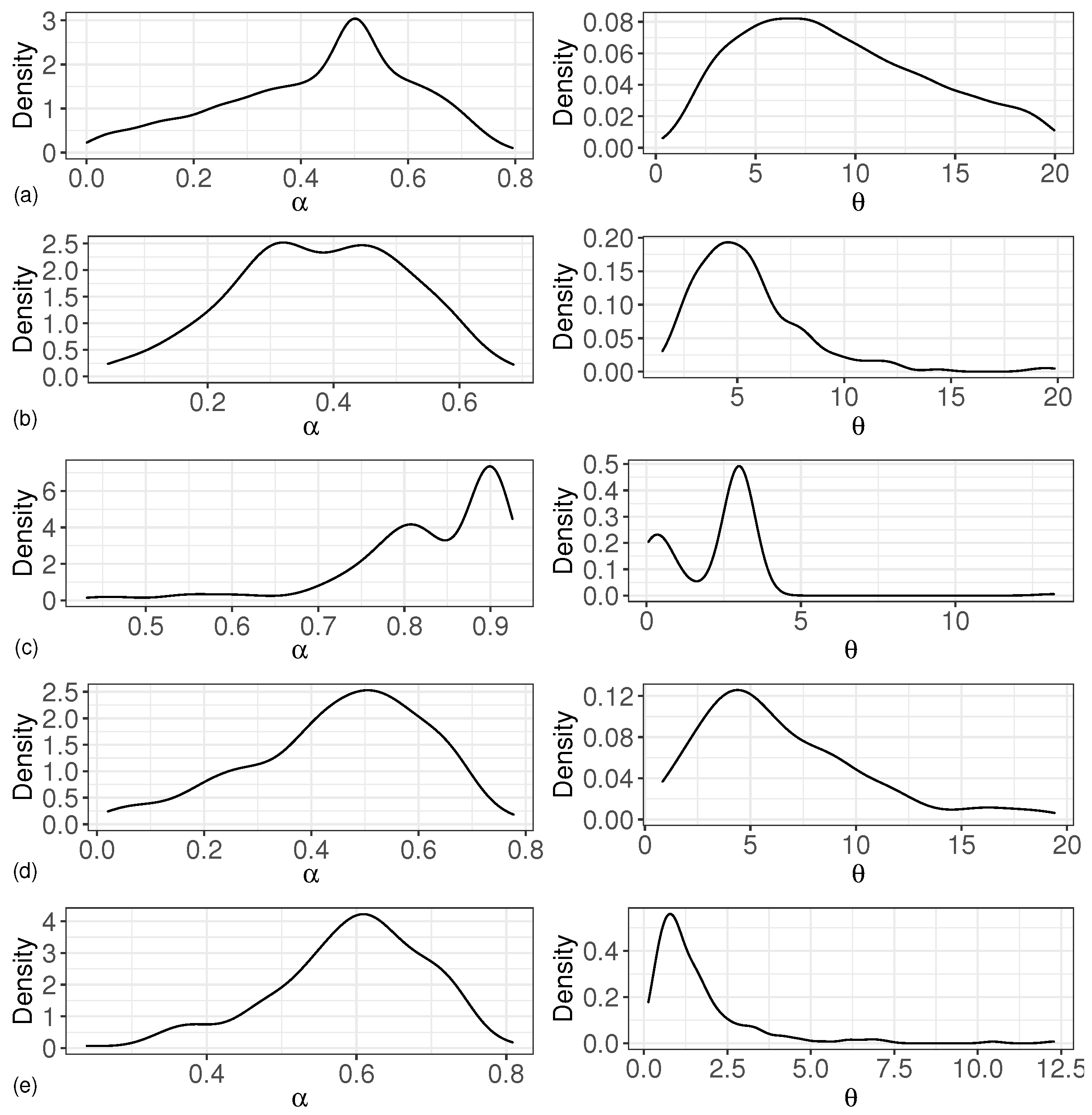
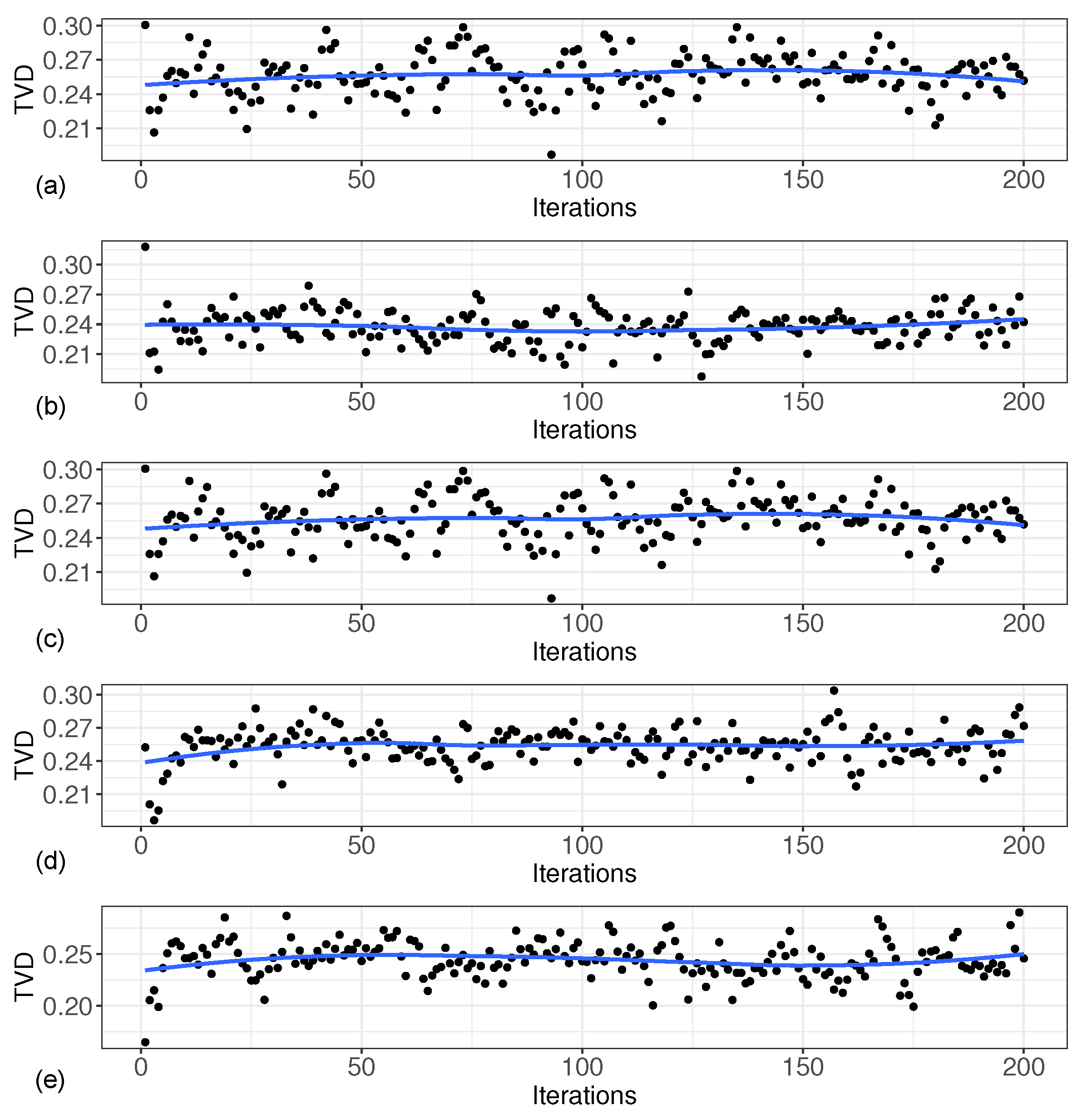
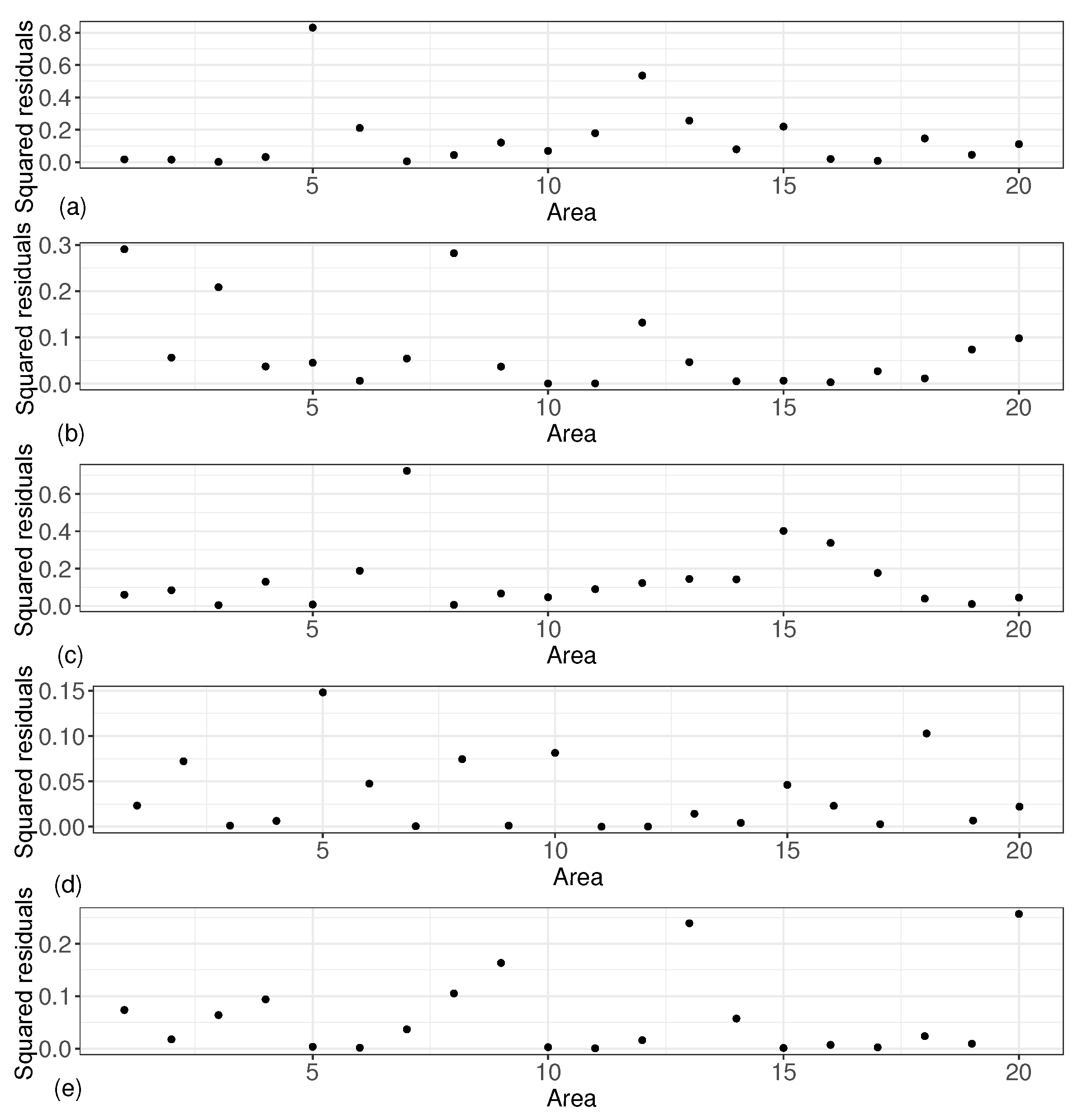
Given the initial values of the parameters and given the full conditional distribution of the MCMC algorithm, we present the sampling stage of the iterative computation. For all $r=0,1,\dots$, with the parameter estimates $\left({\widehat{\alpha }}^{\left(r\right)},{\widehat{\theta }}^{\left(r\right)},{\widehat{h}}_0^{\left(r\right)},{\beta }^{\left(r\right)},{{\sigma }_{\epsilon }^2}^{\left(r\right)}\right)$ already obtained for the rth iteration, we consider sampling from the posterior distribution of the hidden variable ${\nu }_{ij}$. The sampling phase is divided into two steps: the first step is Gibbs sampling based on the full conditional distribution of the MCMC algorithm, and the second step is to consider the use of an accelerated step, that is, to consider the introduction of an auxiliary parameter to sample ${\nu }_{ij}^{*}$ at the end of each iteration. This is because if the sampling is done directly based on the full conditional distribution of the MCMC algorithm, the problem may arise that f and $h_0$ are not conjugate, or the MCMC chain is slow to converge when ${\sum }_{k=1}^{K_i^{-j}}{q}_k$ is relatively large with respect to $q_0$. And, the method of introducing auxiliary parameters can be applied to the two types of problems mentioned above.

To start, we draw ${\nu }_{ij}^b$ from $PD\left({\widehat{\alpha }}^{\left(r\right)},{\widehat{\theta }}^{\left(r\right)};{\widehat{h}}_0^{\left(r\right)}\right)$, for $b=0,1,2,\dots ,B$, where B stands for the number of repetitions within an iteration and is a sufficiently large number. We introduce an auxiliary variable two-step update ${\nu }_{ij}^b$ based on Equation (34), thus referring to the method in the article by Neal [25].

Define the auxiliary variable $c\left({\nu }_i^b\right)=\left(c_1,c_2,\dots ,c_{n_i}\right)$ to denote which category ${\nu }_{ij}^b$ belongs to in ${\nu }_i^{*b}=\left({\nu }_{i1}^{*b},{\nu }_{i2}^{*b},\dots ,{\nu }_{i{K}_i}^{*b},0,\dots ,0\right)$, and use $m^b=\left(m_{i1},m_{i2},\dots ,m_{i{K}_i},0,\dots ,0\right)$ to denote the number of occurrences of ${\nu }_{ij}^b$ in ${\nu }_i^b$. Assuming that ${\nu }_i^b$, $c\left({\nu }_i^b\right)$, ${\nu }_i^{*b}$, and $m^b$ have been obtained, first we consider updating the auxiliary variables first.

For the update of $c_{ij},j=1,2,\dots ,n_i$, suppose that $m_{i{c}_j}=m_{i{c}_j}-1$ if $c_{ij}$ is removed; at this point, $K_i^{-j}=K_i-1$ if $m_{i{c}_j}=0$. Otherwise, the value of $K_i^{-j}$ is the same as that of $K_i$. Then, the new $c_{ij}$ is drawn again, and the distribution of the new $c_{ij}$ is taken as follows:

$$\begin{array}{cc}\hfill q_c& =Pr\left(c_{ij}=c|Y_{ij},c_i^{-j},{\nu }_{i1}^{*},\dots ,{\nu }_{i{K}_i^{-j}}^{*}\right)\hfill \\ & =\left\{\begin{array}{cc}w\left(m_{ic}-{\widehat{\alpha }}^{\left(r\right)}\right)f\left(Y_{ij}|{\nu }_{ic}^{*},{\widehat{\sigma }}_{\epsilon }^{2\left(r\right)},{\widehat{\beta }}^{\left(r\right)}\right),\hfill & 1⩽c⩽n_i,m_{ic}\ne 0\hfill \\ w\left({\widehat{\theta }}^{\left(r\right)}+{\widehat{\alpha }}^{\left(r\right)}{K}_i^{-j}\right)f\left(Y_{ij}|{\nu }_{ic}^{*},{\widehat{\sigma }}_{\epsilon }^{2\left(r\right)},{\widehat{\beta }}^{\left(r\right)}\right),\hfill & 1⩽c⩽n_i,m_{ic}=0\hfill \end{array}\right.\hfill \end{array}$$

(35)

where w is a normalization parameter designed to satisfy the condition ${\sum }_{j=0}^{n_i}{q}_j=1$.

Through the sampling stage, we can obtain ${\nu }_i^b,b=1,2,\dots ,B$. Next, we can estimate the parameters based on the obtained hidden variables ${\nu }_i^b$. We obtain the estimates of each parameter $\left({\tilde{h}}_0\left({\nu }_i^b\right),{\tilde{\sigma }}_{\epsilon }^2\left({\nu }_i^b\right),\tilde{\beta }\left({\nu }_i^b\right),\tilde{\alpha }\left({\nu }_i^b\right),\tilde{\theta }\left({\nu }_i^b\right)\right)$ according to the algorithm mentioned earlier; then, we can obtain the $r+1$th iteration estimates:

$$\left({\widehat{h}}_0^{\left(r+1\right)}\left(·\right),{\widehat{\sigma }}_{\epsilon }^{2\left(r+1\right)},{\widehat{\beta }}^{\left(r+1\right)},{\widehat{\alpha }}^{\left(r+1\right)},{\widehat{\theta }}^{\left(r+1\right)}\right)=\frac{1}{B}\sum _{b=1}^B\left({\tilde{h}}_0\left({\nu }_i^b\right),{\tilde{\sigma }}_{\epsilon }^2\left({\nu }_i^b\right),\tilde{\beta }\left({\nu }_i^b\right),\tilde{\alpha }\left({\nu }_i^b\right),\tilde{\theta }\left({\nu }_i^b\right)\right)$$

(36)

5. Simulation

This section provides the simulation results to study the estimation performance of the proposed parameters under a small area model with PDP randon effects.

5.1. Model Setup and Simulation Conditions

We first design a finite population containing $m=20$ small areas, and we take a certain number of samples in each small area. For convenience, we set the sample capacity of each small area to $n_i=30$.

Then, we provide the following model

$$y_{ij}={\beta }_0+x_{i{j}_1}{\beta }_1+{\nu }_{ij}+{\epsilon }_{ij},j=1,2,\dots ,n_i,i=1,2,\dots ,m$$

(37)

$${\nu }_{i1},\dots ,{\nu }_{i{n}_i}|H_i\stackrel{iid}{\sim }{H}_{i}i=1,2,\dots ,m$$

(38)

$$H_i\sim PD\left(\alpha ,\theta ;H_0\right)$$

(39)

$${\epsilon }_{ij}\sim N\left(0,{\sigma }_{\epsilon }^2\right)j=1,2,\dots ,n_i;i=1,2,\dots ,m$$

(40)

The basic simulation assumptions are as follows:

• Five choices of parameters $\left(\alpha ,\theta \right)$ are: $\left(0.5,10\right)$, $\left(0.3,5\right)$, $\left(0.9,3\right)$, $\left(0.4,7\right)$, or $\left(0.5,2\right)$, and the base distribution is set to be $h_0\sim N\left(0,1\right)$, $h_0\sim t\left(5\right)$, or $h_0\sim t\left(2\right)$;
• The error ${\epsilon }_{ij}$ comes from a normal distribution $N\left(0,0.1^2\right)$;
• The true value of the regression coefficient is set to $\beta ={\left({\beta }_0,{\beta }_1\right)}^{\prime }={\left(1,2\right)}^{\prime }$;
• The initial parameter values $\left({\widehat{\alpha }}^{\left(0\right)},{\widehat{\theta }}^{\left(0\right)}\right)$ are set to be $\left(0.2,5\right)$, $\left(0.2,2\right)$, $\left(0.5,1\right)$, $\left(0.1,5\right)$, or $\left(0.1,1\right)$ when $\left(\alpha ,\theta \right)$ is $\left(0.5,10\right)$, $\left(0.3,5\right)$, $\left(0.9,3\right)$, $\left(0.4,7\right)$, or $\left(0.5,2\right)$;
• The initial random effects are set to ${\widehat{\nu }}_{ij}^{\left(0\right)}=y_{ij}$;
• The number of iterations for the MCMC algorithm is set to $R=200$.

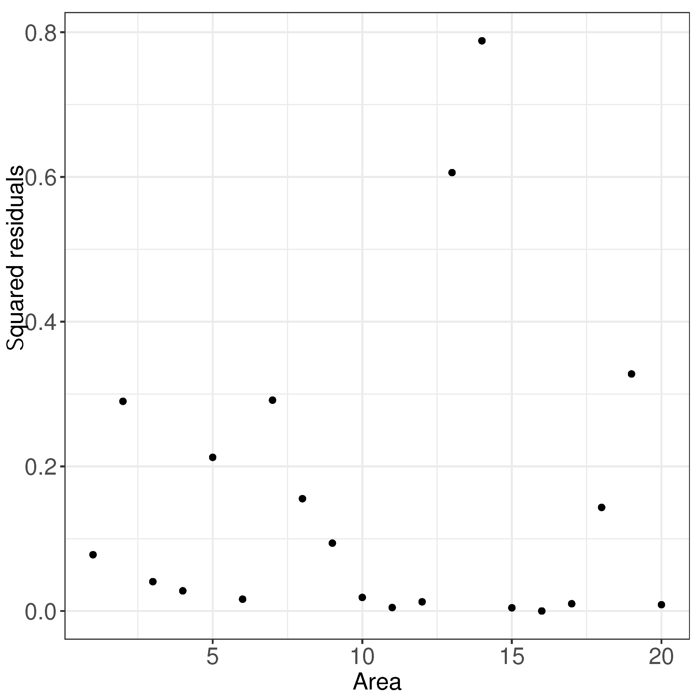
5.2. Simulation Results and Analysis

The simulation results are given in detail by the following figures and tables. Table 1 shows the simulation results of the estimation of the corresponding parameters for the different cases of varying the values of parameters $\alpha$ and $\theta$ versus transforming the base distribution under the PDP prior for random effects in the proposed model. The first column in Table 1 shows all the parameters that were estimated, the second column shows the settings of the base distribution for the different cases, the third column shows the true values of the corresponding parameters, the fourth and fifth columns show the bias and the MSE, and the sixth column shows the 95 percent confidence domain. Figure 1 shows the density estimation curves for the parameters $\alpha$ and $\theta$ under different simulation data.

Table 1. Performance of parameters estimation.

Parameter	Base Distribution	True Value	Bias	MSE	Confidence Interval
$\alpha$	$N\left(0,1\right)$	0.5	−0.06534407	0.03458486	(0.427019, 0.442293)
$\theta$		10	−0.9001747	22.34711	(8.874574, 9.325077)
${\beta }_0$		1	0.01457439	0.005534238	(1.011374, 1.017774)
${\beta }_1$		2	0.03045286	0.01246042	(2.025742, 2.035163)
$\alpha$	$N\left(0,1\right)$	0.3	0.08081297	0.02533613	(0.361643, 0.399983)
$\theta$		5	0.4856122	7.561553	(5.105321, 5.865904)
${\beta }_0$		1	0.01848704	0.002993466	(1.011289, 1.025685)
${\beta }_1$		2	0.04352289	0.004664257	(2.036166, 2.050880)
$\alpha$	$N\left(0,1\right)$	0.9	−0.07212803	0.01389355	(0.814840, 0.840904)
$\theta$		3	−0.8307739	3.068224	(1.915222, 2.423231)
${\beta }_0$		1	0.08176262	0.01210896	(1.071468, 1.092058)
${\beta }_1$		2	−0.08813282	0.01125358	(1.903614, 1.920121)
$\alpha$	$t\left(5\right)$	0.4	0.05213893	0.02911436	(0.429428, 0.474850)
$\theta$		7	−0.5294164	15.58317	(5.916658, 7.024509)
${\beta }_0$		1	0.06114231	0.006702937	(1.053531, 1.068753)
${\beta }_1$		2	0.02870615	0.004429664	(2.020312, 2.037100)
$\alpha$	$t\left(2\right)$	0.5	0.09099937	0.01867303	(0.576749, 0.605250)
$\theta$		2	−0.3801979	2.727176	(1.395155, 1.844450)
${\beta }_0$		1	−0.1348095	0.02203277	(0.856507, 0.873875)
${\beta }_1$		2	0.3587933	0.1333754	(2.349268, 2.368318)

Figure 1. Density estimation curve of $\alpha$ and $\theta$. (a) $\left(\alpha ,\theta \right)=\left(0.5,10\right)$ based on $N\left(0,1\right)$; (b) $\left(\alpha ,\theta \right)=\left(0.3,5\right)$ based on $N\left(0,1\right)$; (c) $\left(\alpha ,\theta \right)=\left(0.9,3\right)$ based on $N\left(0,1\right)$; (d) $\left(\alpha ,\theta \right)=\left(0.4,7\right)$ based on $t\left(5\right)$; (e) $\left(\alpha ,\theta \right)=\left(0.5,2\right)$ based on $t\left(2\right)$.

In Table 1, we calculated the bias, MSE, and confidence intervals of $\widehat{\alpha }$ and $\widehat{\theta }$ for different types of base distributions. We assumed that the base distribution follows the normal distribution $N\left(0,1\right)$ and the t distribution, respectively. Here, we chose t distributions with five and two degrees of freedom as the base distributions for estimation. The results of these estimators obtained under two different types of base distribution conditions were similar. The biases of $\widehat{\alpha }$ were inside the interval $\left(-0.073,0.091\right)$, and the biases of $\widehat{\theta }$ were inside the interval $\left(-0.901,0.486\right)$. The MSEs of $\widehat{\alpha }$ were less than 0.04, although the MSEs of $\widehat{\alpha }$ were large, and most of the estimated confidence intervals failed to capture the true values of the parameters. Meanwhile, we considered the bias, MSE, and confidence intervals of $\widehat{\alpha }$ and $\widehat{\theta }$ with different true values for $\alpha$ and $\theta$ under the condition where the base distribution follows a normal distribution or a t distribution. From Table 1, we can see that when the base distribution followed the normal distribution and $\left(\alpha ,\theta \right)=\left(0.5,10\right)$, the bias and MSE of $\widehat{\theta }$ were larger than those of other cases. The bias and MSE of $\widehat{\theta }$ were the smallest when the base distribution followed $t\left(2\right)$ and $\left(\alpha ,\theta \right)=\left(0.5,2\right)$. The density curve of $\widehat{\alpha }$ and $\widehat{\theta }$ in Figure 1 also agrees with the estimated results of Table 1.

Table 1 lists the estimation results of the regression coefficients given different values of the parameters $\alpha$ and $\theta$ and different base distribution conditions. The biases and MSEs of ${\beta }_0$ and ${\beta }_1$ were maintained at very low levels, which reflect the accuracy and reliability of the estimates. Figure 2 shows the density estimation curve of ${\beta }_0$ and ${\beta }_1$ when $\left(\alpha ,\theta \right)=\left(0.5,10\right)$ based on $N\left(0,1\right)$, which coincides with the estimation results in Table 1.

Figure 2. Density estimation curve of regression coefficients when $\left(\alpha ,\theta \right)=\left(0.5,10\right)$ based on $N\left(0,1\right)$.

Table 2 presents the results of a comparison between the estimates of the regression coefficients ${\beta }_0$ and ${\beta }_1$ of the proposed model and those of the NER model, as derived from five sets of simulations. Table 2 demonstrates that the estimates of ${\beta }_0$ and ${\beta }_1$ obtained from the estimation of both the proposed model and the NER model were highly close to the true values. However, for the simulation where the base distribution followed the normal distribution, the NER model estimation was slightly more accurate than the proposed model. Conversely, when the base distribution followed the t distribution, the proposed model estimation was more precise than the NER model estimation.

Table 2. Estimated mean of regression coefficients.

Regression Coefficient	True Value	NER Model	NER Model with PDP Random Effects
		0.9607364	1.014574
		1.017708	1.018487
${\beta }_0$	1	1.001620	1.081763
		1.069568	1.061142
		0.7113994	0.8651905
		2.045244	2.030453
		2.038286	2.043523
${\beta }_1$	2	1.900959	1.911867
		2.044987	2.028706
		2.4582498	2.358793

The Total Variation Distance (TVD) is a statistical distance measure between probability distributions, which represents the distance between the true and estimated distribution of the base distribution $h_0$ and thus serves as a basis for evaluating the estimation performance. Figure 3 shows the Total Variation Distance between the two distributions for each iteration under these five scenarios. As can be seen from Figure 3, the gap between the estimated distribution and the true distribution was small, and the total variance distance was less than 0.3 in each iteration.

Figure 3. Total variation distance between two distributions at each iteration. (a) $\left(\alpha ,\theta \right)=\left(0.5,10\right)$ based on $N\left(0,1\right)$; (b) $\left(\alpha ,\theta \right)=\left(0.3,5\right)$ based on $N\left(0,1\right)$; (c) $\left(\alpha ,\theta \right)=\left(0.9,3\right)$ based on $N\left(0,1\right)$; (d) $\left(\alpha ,\theta \right)=\left(0.4,7\right)$ based on $t\left(5\right)$; (e) $\left(\alpha ,\theta \right)=\left(0.5,2\right)$ based on $t\left(2\right)$.

Table 3 shows the simulation results for the estimates of all small area means ${\rho }_i$ when the situation was that $\left(\alpha ,\theta \right)=\left(0.5,10\right)$ and the base distribution is $N\left(0,1\right)$. The first column in Table 3 shows the mean of ${\rho }_i$, and the second column is the estimated value of the small area mean. As can be seen from Table 3, the estimates about the small area means were more accurate, and the estimates were close to the means without large deviations.

Table 3. Results of small areas means when $\left(\alpha ,\theta \right)=\left(0.5,10\right)$ based on $N\left(0,1\right)$.

Area	Sample Mean	Estimate
1	2.089628	2.220492
2	1.793437	1.916604
3	1.692420	1.731447
4	2.428903	2.606485
5	1.550903	2.462545
6	2.068002	2.527393
7	2.412526	2.482989
8	1.717398	1.926363
9	2.042811	2.390698
10	2.094958	2.358032
11	2.218328	2.641435
12	1.865992	2.597315
13	1.725139	2.231473
14	2.020898	2.302906
15	1.630873	2.099237
16	2.129673	2.268741
17	1.834107	1.922384
18	2.570386	2.952974
19	2.006835	2.219573
20	1.733093	2.066331

In order to more directly reflect the reliability of the estimation of the small area means, we introduced squared residuals to measure the degree of matching between the estimated values of the small area means and the true values, and we give five graphs of the squared residuals of the small area means under these five scenarios. As shown in Figure 4, the squared residuals for all small area means were small, with most of the squared residuals centered between 0 and 0.3.

Figure 4. Squared residuals results of small area means. (a) $\left(\alpha ,\theta \right)=\left(0.5,10\right)$ based on $N\left(0,1\right)$; (b) $\left(\alpha ,\theta \right)=\left(0.3,5\right)$ based on $N\left(0,1\right)$; (c) $\left(\alpha ,\theta \right)=\left(0.9,3\right)$ based on $N\left(0,1\right)$; (d) $\left(\alpha ,\theta \right)=\left(0.4,7\right)$ based on $t\left(5\right)$; (e) $\left(\alpha ,\theta \right)=\left(0.5,2\right)$ based on $t\left(2\right)$.

5.3. Simulated Normal Data

In this section, we demonstrated how we implemented the estimation by using simulated data with the aim of testing the strengths and weaknesses of the model. Similar to the simulations in the previous section and for ease of computation, we assumed that there are $m=20$ small areas, and the sample size for each small area was set to $n_i=30$. And, the simulation data $y_{ij}$ were derived from the following model structure:

$$y_{ij}={\beta }_0+x_{i{j}_1}{\beta }_1+{\nu }_{ij}+{\epsilon }_{ij},j=1,2,\dots ,n_i;i=1,2,\dots ,m$$

(41)

$${\nu }_{ij}\sim N\left(0,{\sigma }_{\nu }^2\right)j=1,2,\dots ,n_i;i=1,2,\dots ,m$$

(42)

$${\epsilon }_{ij}\sim N\left(0,{\sigma }_{\epsilon }^2\right)j=1,2,\dots ,n_i;i=1,2,\dots ,m$$

(43)

where the random effects ${\nu }_{ij}$ comes from a normal distribution $N\left(0,4\right)$, and the error ${\epsilon }_{ij}$ comes from a normal distribution $N\left(0,0.1^2\right)$. The true value of the regression coefficient was set to $\beta ={\left({\beta }_0,{\beta }_1\right)}^{\prime }={\left(1,2\right)}^{\prime }$.

Then, we used the proposed model with PDP random effects to estimate and obtain the corresponding estimates. Table 4 shows the results of parameter estimation. The estimates of the fixed effects in Table 4 were very close to the true values, and through Table 4, we can also observe the parameters $\alpha$ and $\theta$ of the PDP prior for the random effects of the model. Based on the estimates of the parameters $\alpha$ and $\theta$ and the estimated distribution of the base distribution of the random effects, we further obtained the estimates of the means of all the small areas through the model, which are presented through Table 5. Table 5 shows that the estimation of the small area mean was more reliable, and the estimates were close to the means without major deviations. Figure 5 shows squared residuals for all the small area means. We can find that the residual squared of all small area means were small, thus demonstrating the validity of our model and method.

Table 4. Performance of parameters estimation of simulated data.

$\widehat{\mathit{\alpha }}$	$\widehat{\mathit{\theta }}$	${\widehat{\mathit{\beta }}}_0$	${\widehat{\mathit{\beta }}}_1$
0.6003261	5.124903	1.003003	2.411909

Table 5. Results of small areas means of simulated data.

Area	Sample Mean	Estimate
1	2.6218905	2.342866
2	2.0078687	1.469475
3	0.9612582	1.162803
4	1.5513356	1.384326
5	2.2699821	1.809038
6	2.0796827	1.951780
7	3.0264584	2.486590
8	3.1521868	2.758094
9	1.2477416	1.554100
10	1.2796926	1.416766
11	2.5728659	2.642539
12	1.8507724	1.963746
13	2.8604333	2.081979
14	3.1778784	2.290092
15	1.7505182	1.817446
16	1.8190648	1.810704
17	1.0271540	1.127514
18	2.6706406	2.292215
19	2.5922461	2.019817
20	2.7200485	2.626496

Figure 5. Squared residuals results of small area means of simulated data.

6. Application

Following this, we applied the proposed model to a dataset of combined income and other sociological variables for the Spanish provinces [26], which is available in the R package sae [27]. This dataset contains 20 regions, 21 variables, and a total of 1050 observation units. We retained and integrated these variables to select four variables, that is, incomedata, age, edu, and sex, thus representing total income, age, education level, and gender, respectively. Because the central aim of the survey was to understand the income levels of the Spanish provinces, incomedata was used directly as a response variable in the model. The remaining three variables, age, edu, and sex, are considered to be closely related to income and therefore served as auxiliary variables in the model. We removed any units containing missing values in these variables and normalized these data.

The proposed model can be described as follows:

$$incomedat{a}_{ij}={\beta }_0+{\beta }_{1}ed{u}_{ij}+{\beta }_{2}se{x}_{ij}+{\beta }_{3}ag{e}_{ij}+{\nu }_{ij}+{\epsilon }_{ij},j=1,2,\dots ,n_i;i=1,2,\dots ,m$$

(44)

$${\nu }_{i1},\dots ,{\nu }_{i{n}_i}|H_i\stackrel{iid}{\sim }{H}_{i}i=1,2,\dots ,m$$

(45)

$$H_i\sim PD\left(\alpha ,\theta ;h_0\right)$$

(46)

$${\epsilon }_{ij}\sim N\left(0,{\sigma }_{\epsilon }^2\right)j=1,2,\dots ,n_i;i=1,2,\dots ,m$$

(47)

Based on the proposed model, by applying the parameter estimation method in Section 4 and the provided algorithm to run two hundred rounds, the estimation results of each parameter were obtained and are shown in Table 6. Figure 6 gives the density plot of the base distribution obtained from our estimation.

Table 6. Performance of parameters estimation of real data.

$\widehat{\mathit{\alpha }}$	$\widehat{\mathit{\theta }}$	${\widehat{\mathit{\beta }}}_0$	${\widehat{\mathit{\beta }}}_1$	${\widehat{\mathit{\beta }}}_2$	${\widehat{\mathit{\beta }}}_3$
0.875775	3.025505	−0.007919	−0.000048	−0.000173	−0.000169

Figure 6. Density of estimated base distribution of real data.

7. Conclusions

In this paper, we proposed to use the Poisson–Dirichlet Process in a Nested Error Regression model to provide a priori distributions for random effects in unit-level data. In the small area model, since the random effects are not directly observable as hidden variables, we applied the MCMC algorithm to extract the random effects at fixed initial values and constructed parameter estimates in the prior; we then gave estimates of the parameters such as regression coefficients and the base distributions with known random effects. Through numerical simulations and the application of example data, we demonstrated the feasibility of the studied model and the practicality of the estimation algorithm.

Our proposed model and its parameter estimation method have significant advantages. Firstly, the Poisson–Dirichlet process as a prior is able to flexibly capture the nonparametric properties of the random effects, thus overcoming the limitations of the traditional normality assumption and improving the adaptability and accuracy of the model. Second, the effective application of the MCMC algorithm ensures the robustness and accuracy of parameter estimation, especially when dealing with complex data and models. Both the theoretical and simulation results confirm these advantages, thus making our model and method widely applicable and effective in practical applications.

Although our proposed model and method performed well in several aspects, there are still some shortcomings and directions worthy of further research. The computational complexity of the models is high, especially when dealing with large-scale datasets, and the computational cost may become a limiting factor for their application. Therefore, developing more efficient computational methods and algorithms is a future research focus. In addition, with the development of data science, combining new statistical techniques and machine learning algorithms to improve and optimize the model is also a worthy research direction.

References

- Rao, J.N. Small Area Estimation; John Wiley & Sons: Hoboken, NJ, USA, 2005; Volume 331. [Google Scholar]
- Pfeffermann, D. New important developments in small area estimation. Stat. Sci. 2013, 28, 40–68. [Google Scholar] [CrossRef]
- Rao, J.N.; Molina, I. Small Area Estimation; John Wiley & Sons: Hoboken, NJ, USA, 2015. [Google Scholar]
- Fay, R.E., III; Herriot, R.A. Estimates of income for small places: An application of James-Stein procedures to census data. J. Am. Stat. Assoc. 1979, 74, 269–277. [Google Scholar] [CrossRef]
- Battese, G.E.; Harter, R.M.; Fuller, W.A. An error-components model for prediction of county crop areas using survey and satellite data. J. Am. Stat. Assoc. 1988, 83, 28–36. [Google Scholar] [CrossRef]
- Arima, S.; Bell, W.R.; Datta, G.S.; Franco, C.; Liseo, B. Multivariate Fay–Herriot Bayesian estimation of small area means under functional measurement error. J. R. Stat. Soc. Ser. A Stat. Soc. 2017, 180, 1191–1209. [Google Scholar] [CrossRef]
- Yang, Z.; Chen, J. Small area mean estimation after effect clustering. J. Appl. Stat. 2020, 47, 602–623. [Google Scholar] [CrossRef] [PubMed]
- Datta, G.S.; Hall, P.; Mandal, A. Model selection by testing for the presence of small-area effects, and application to area-level data. J. Am. Stat. Assoc. 2011, 106, 362–374. [Google Scholar] [CrossRef]
- Sugasawa, S.; Kubokawa, T. Bayesian estimators in uncertain nested error regression models. J. Multivar. Anal. 2017, 153, 52–63. [Google Scholar] [CrossRef]
- Ferrante, M.R.; Pacei, S. Small domain estimation of business statistics by using multivariate skew normal models. J. R. Stat. Soc. Ser. A Stat. Soc. 2017, 180, 1057–1088. [Google Scholar] [CrossRef]
- Fabrizi, E.; Trivisano, C. Robust linear mixed models for small area estimation. J. Stat. Plan. Inference 2010, 140, 433–443. [Google Scholar] [CrossRef]
- Chakraborty, A.; Datta, G.S.; Mandal, A. A two-component normal mixture alternative to the Fay-Herriot model. Stat. Transit. New Ser. 2016, 17, 67–90. [Google Scholar]
- Diallo, M.S.; Rao, J. Small area estimation of complex parameters under unit-level models with skew-normal errors. Scand. J. Stat. 2018, 45, 1092–1116. [Google Scholar] [CrossRef]
- Tsujino, T.; Kubokawa, T. Empirical Bayes methods in nested error regression models with skew-normal errors. Jpn. J. Stat. Data Sci. 2019, 2, 375–403. [Google Scholar] [CrossRef]
- Opsomer, J.D.; Claeskens, G.; Ranalli, M.G.; Kauermann, G.; Breidt, F.J. Non-parametric small area estimation using penalized spline regression. J. R. Stat. Soc. Ser. B Stat. Methodol. 2008, 70, 265–286. [Google Scholar] [CrossRef]
- Polettini, S. A Generalised Semiparametric Bayesian Fay–Herriot Model for Small Area Estimation Shrinking Both Means and Variances. Bayesian Anal. 2016, 12, 729–752. [Google Scholar] [CrossRef]
- Pitman, J.; Yor, M. The two-parameter Poisson-Dirichlet distribution derived from a stable subordinator. Ann. Probab. 1997, 25, 855–900. [Google Scholar] [CrossRef]
- Al-Labadi, L.; Hamlili, M.; Ly, A. Bayesian Estimation of Variance-Based Information Measures and Their Application to Testing Uniformity. Axioms 2023, 12, 887. [Google Scholar] [CrossRef]
- Handa, K. The two-parameter Poisson–Dirichlet point process. Bernoulli 2009, 15, 1082–1116. [Google Scholar] [CrossRef]
- Favaro, S.; Lijoi, A.; Mena, R.H.; Prünster, I. Bayesian non-parametric inference for species variety with a two-parameter Poisson–Dirichlet process prior. J. R. Stat. Soc. Ser. B Stat. Methodol. 2009, 71, 993–1008. [Google Scholar] [CrossRef]
- Gelman, A.; Carlin, J.B.; Stern, H.S.; Rubin, D.B. Bayesian Data Analysis, 3rd ed.; Chapman and Hall/CRC: Boca Raton, FL, USA, 2013. [Google Scholar]
- Yang, L.; Wu, X. Estimation of Dirichlet process priors with monotone missing data. J. Nonparametr. Stat. 2013, 25, 787–807. [Google Scholar] [CrossRef]
- Qiu, X.; Yuan, L.; Zhou, X. MCMC sampling estimation of Poisson-Dirichlet process mixture models. Math. Probl. Eng. 2021, 2021, 6618548. [Google Scholar] [CrossRef]
- Carlton, M.A. Applications of the Two-Parameter Poisson-Dirichlet Distribution; University of California: Los Angeles, CA, USA, 1999. [Google Scholar]
- Neal, R.M. Markov chain sampling methods for Dirichlet process mixture models. J. Comput. Graph. Stat. 2000, 9, 249–265. [Google Scholar] [CrossRef]
- Molina, I.; Rao, J.N. Small area estimation of poverty indicators. Can. J. Stat. 2010, 38, 369–385. [Google Scholar] [CrossRef]
- Molina, I.; Marhuenda, Y. sae: An R Package for Small Area Estimation. R J. 2015, 7, 81–98. [Google Scholar] [CrossRef]
Disclaimer/Publisher’s Note: The statements, opinions and data contained in all publications are solely those of the individual author(s) and contributor(s) and not of MDPI and/or the editor(s). MDPI and/or the editor(s) disclaim responsibility for any injury to people or property resulting from any ideas, methods, instructions or products referred to in the content. |
© 2024 by the authors. Licensee MDPI, Basel, Switzerland. This article is an open access article distributed under the terms and conditions of the Creative Commons Attribution (CC BY) license (https://creativecommons.org/licenses/by/4.0/).