Abstract
In clinical studies focusing on paired body parts, diseases can manifest on either both sides (bilateral) or just one side (unilateral) of the organs. Consequently, the data in these studies may consist of records from both bilateral and unilateral cases. There are two different methods of analyzing the data. One of the methods is assuming that the pair of measurements from the same subject are independent, while the other considers the correlation between paired organs. In terms of the homogeneity test of proportions, asymptotic methods have been proposed given the moderate size of data. This article extends the existing work by proposing exact methods to deal with the scenarios when the sample size is small and asymptotic methods perform poorly. The impact of the correlation assumption is also explored. Among the proposed methods, calculating p-values by replacing unknown parameters with estimated values while accounting for the correlation is recommended based on its satisfactory type I error controls and statistical powers. The proposed methods are applied to three real examples for illustration.
Keywords:
equal correlation coefficients model; homogeneity test; unilateral and bilateral data; exact method MSC:
62F03
1. Introduction
Data collected from paired organs of human bodies can be bilateral or unilateral depending on the availability of each site or the disease status. Whether to assume or ignore the correlation between two sites of an organ remains an interesting discussion. The majority of articles published in the British Journal of Ophthalmology (BJO) in 1995 and 2017 assumed independence of the sites according to Zhang and Ying [1]. For the homogeneity tests of group-specific response rates given the outcome is binary, classical methods such as Pearson’s chi-squared test [2] can be applied. However, Rosner [3], Donner, and Banting [4]) criticized this approach by pointing out that the omission of the correlation will lead to biased inferences. However, there are not many studies that demonstrate such a bias with numerical presentations.
To avoid the possible bias, Donner [5] assumed that the number of successes from each pair of organs follows a binomial distribution with probability parameter P, where P varies among subjects and has an expectation of p. The variance of P is proportional to ; that is, . This concept can be extended easily by assuming the intra-person correlation is , where ranges from to 1. The correlation is assumed to be constant for all individuals and is referred to as the equal correlation coefficients model. In the context of bilateral data, Ma and Liu [6] derived three asymptotic methods, the likelihood ratio test, the score test, and the Wald-type test, to assess the homogeneity of prevalences of multiple groups. Mou and Li [7] compared multiple algorithms for estimating parameters and investigated asymptotic statistics for the homogeneity test of many-to-one risk differences. Liu et al. [8] considered four exact approaches, the E approach, the M approach, the E + M approach, and the C approach, as alternatives to the methods proposed by Ma and Liu [6] when the sample size cannot ensure a good asymptotic approximation. In general, exact approaches calculate the probability of a tail area, which is defined as a set of cases that are more extreme than the observed data against the null hypothesis. The E approach, initially proposed by Liddell [9], replaces nuisance parameters with their corresponding maximum likelihood estimate. Basu [10] introduced the M approach, which involves determining the p-value by maximizing the likelihood of observing the tail area across the entire parameter space. By combining the E and the M methods, Lloyd [11] first determined the tail area by regarding the p-value from the E approach as a statistic and then applied the M method to calculate the final p-value. The previous three methods assume the group totals are fixed, while the C method in Liu’s work [8] fixes both margins of a table. In the context of bilateral and unilateral combined data, Ma and Wang [12] derived three asymptotic approaches for testing the equality of proportions using the equal correlation coefficients model. It is worth noting that these methods still require a large sample size, and there is a need to extend Liu’s work to combined data.
This article proposes five exact approaches given bilateral and unilateral combined data with limited samples for testing the equivalence of proportions of multiple groups. Section 2 presents details of Donner’s equal correlation coefficients model. In Section 3, we introduce the individual site model, which omits the correlation between sites. Classical methods based on the individual site model are described in Section 4, and we introduce five exact approaches in Section 5 using Donner’s model. In Section 4, we provide numerical studies that compare the two models and various methods with regard to their ability to control Type I errors (TIEs) and their statistical powers. The application of the proposed methods through two real-world examples is illustrated in Section 6. The final conclusions and discussion are given in Section 7.
2. Equal Correlation Coefficients Model
Define as the event of the jth subject in the ith group having a response at the kth site and as , where and . The equal correlation coefficients model proposed by Donner [5] assumes the correlation coefficient between measurements from two sites to be a constant . In the bilateral cohort where subjects contribute one measurement at each site of the paired organs, let stand for the number of subjects with r response(s) in the ith group, where . In the unilateral cohort where subjects provide one measurement on only one site of the paired organs, denotes the number of subjects with response(s) in the ith group, where . The data layout on the subject level can be found in Table 1.

Table 1.
Data layout on subject level.
Given the nature of clinical study designs, are fixed, and the plausible distribution assumptions are as follows:
In observational studies, the sample size of each group can be random, which is beyond the scope of this article. It can be easily shown that , , , , and . The null and the alternative hypotheses of interest are as follows:
3. Individual Site Model without Considering Correlation
Many studies encounter challenges due to the limited sample size of participants. One of the common strategies that researchers consider is conducting analyses on the site level of each subject to extract as much information as possible. To our knowledge, the impact of ignoring the potential correlation of the two sites of a subject remains unknown. In order to explore this effect, data from the equal correlation coefficients model are transformed to new data on the site level. Define as the number of sites with e response, where and . The new data structure is presented in Table 2. The relationship between the two types of data is presented as follows:

Table 2.
Data layout on site level.
The random variables and are assumed to follow binomial distributions Bin() and Bin(), respectively. The null and the alternative hypotheses are the same as stated in Section 2.
4. Methods for Individual Site Model
4.1. The Pearson Chi-Squared Test
Define the notation as an observed table from Table 2. Given the ignorance of correlations between the sites, the individual site model becomes an unordered table where the Pearson chi-squared test statistic is given by Equation (1).
The p-value is defined as since the test statistic asymptotically follows a chi-squared distribution with degrees of freedom when the sample size is sufficient (Fagerland et al. [13]). The null hypothesis is rejected if the calculated p-value is less than 0.05 given the significance level of 0.05.
4.2. The Fisher–Freeman–Halton Exact Test
The asymptotic behavior described above does not hold when the numbers in Table 2 are small. To overcome this limitation, an alternative test called the Fisher–Freeman–Halton (FFH) exact test can be employed (Fagerland et al. [13]). The point probability, , conditions both the row and column totals and is used as the test statistic. In the null hypothesis, the probability distribution of Table 2 follows the multiple hypergeometric distribution. The Fisher–Freeman–Halton exact test treats tables with a smaller point probability than as a piece of evidence against , where is the probability of observing . Let represent the collection of all tables sharing the same row and column margins as the observed table . Therefore, the exact p-value is defined by Equation (2), where is the indicator function.
4.3. The Mid-P Test
The Fisher–Freeman–Halton exact test is often criticized for being unnecessarily conservative due to discreteness in certain scenarios. One of the adjustments to is called the mid-P test. This test downsizes the weight of tables with the same point probability as the observed table (Fagerland et al. [13]). In other words, the adjusted p-value can be defined by Equation (3).
5. Methods for Equal Correlation Coefficients Model
Given observed data , the likelihood function is given by Equation (4), and the log-likelihood function can be written as a function of and as shown in Equation (5).
Let represent for ease of notation. With , the maximum likelihood estimates (MLEs) can be obtained by setting the partial derivatives with respect to and to zero and solving Equations (6) and (7).
Let and denote the constrained MLEs for . The closed-form solutions to the above equations can be found in Ma and Wang’s work [12].
5.1. Score Test
Ma and Wang [12] examined the likelihood ratio test, the score test, and the Wald-type test and concluded that the score test outperformed the other two approaches based on simulation studies using various combinations of parameter settings and sample sizes. Therefore, we choose the score test to explore the asymptotic behaviors given smaller sample sizes compared to Ma and Wang’s settings. This approach is referred to as the A method. The score test statistic is given by Equation (8), where , and is the Fisher information assuming the group-specific proportion ’s.
We kindly recommend that readers refer to Ma and Wang’s work for a simplified form of . Asymptotically, the score test statistic follows a chi-square distribution with degrees of freedom given the null hypothesis is true according to Rao [14]. The corresponding p-value can be calculated by Equation (9).
Similar to the Pearson chi-squared statistic, the approximation to does not hold if the sample size is insufficient, leading to uncontrolled type I error rates. To alleviate this difficulty, four exact methods are proposed by fixing and are described in detail in Section 5.2, Section 5.3, Section 5.4 and Section 5.5. Define the collection of all tables with the same row margin as in Table 1 as . In Section 5.6, we propose another exact method by fixing both the row and column totals.
5.2. E Method
There are several methods to calculate p-values based on the summation of probabilities of tables that are more extreme than the observed table when is true. One of the approaches treats the values of constrained MLEs and as the true parameter values, and it is referred to as the E method because these estimates are used as substitutes for unknown parameters in calculations. As a result, the p-value based on the E method is defined by Equation (10).
5.3. M Method
Instead of using the estimated parameters directly, an alternative approach is to maximize the above summation of probabilities in the whole parameter space. This technique is denoted as the M method. The exact p-value can be calculated by Equation (11).
5.4. E + M Method
The M method discussed above calculates p-values based on the score test statistic. Notice that the exact p-value, , can be regarded as a statistic as well and replace the role of the score statistic in the M method. The fusion of the two approaches is referred to as the E + M method. The exact p-value is defined by Equation (12).
5.5. CI Method
Unlike the M method, a smaller parameter space consisting of the confidence intervals (CIs) of and can be used when maximizing the summation of probabilities, and this is called the CI method. The confidence intervals of and are denoted as and , respectively. We kindly ask the readers to refer to Berger [15] and Silvapulle’s [16] work for details. In essence, the rationale is that the M method can be conservative since the generated p-values may be close to one due to the nature of the supremum. The CI method shrinks the parameter space, resulting in smaller p-values than the M approach. The corresponding p-value is defined by Equation (13).
A definition of the p-value is considered valid if p-value holds according to Vexler [17]). A simple proof that is a valid p-value is given in the Appendix A.
The confidence intervals of and are derived using another score test statistic () with the null hypothesis . The conditional MLE of given known can be obtained by solving Equation (2), and the conditional MLE of given can be obtained by solving Equation (1). The score test statistic can be expressed by Equation (14),
where
The following iterative procedure outlines the details of finding the upper limit of the CI of :
- (1)
- Set as the starting point of , where is the constrained MLE of for . Initialize flag = 1 and stepsize = so that the updated upper bound does not prematurely exceed 1;
- (2)
- Update + flag × stepsize and calculate the conditional MLE given . Then, the score test statistic is given by ;
- (3)
- If , where is the quantile of the chi-square distribution with one degree of freedom, turn to the opposite searching direction by letting flag = −1 and reduce the stepsize by multiplying it by , then return to step (2). Otherwise, keep flag = 1 and return to step (2);
- (4)
- Repeat steps (2) and (3) until the stepsize is sufficiently small (e.g., ).
The lower limit of the CI of can be determined by letting flag = −1 and stepsize = in step (1) and then multiplying it by −1 if or multiplying it by 1 if .
The following procedures can be used to determine the upper limit of the CI of :
- (1)
- Set as the starting point of , where is the constrained MLE of for . Initialize flag = 1 and stepsize = ;
- (2)
- Update + flag × stepsize and calculate the conditional MLE given . Then, the score test statistic is given by ;
- (3)
- If , turn to the opposite searching direction by letting flag = −1 and reduce the stepsize by multiplying it by , then return to step (2). Otherwise, keep flag = 1 and return to step (2);
- (4)
- Repeat steps (2) and (3) until the stepsize is sufficiently small (e.g., ).
The lower bound of the CI of can be found by initializing flag = −1 and stepsize = in step (1) and multiply it by −1 if or multiply it by 1 if .
5.6. C Method
The conditional method, denoted as the C method, assumes both the column and row totals are fixed in Table 1, and it does not involve nuisance parameters in determining p-values. Let represent the margins of the observed table and define as the collection of all tables having the same margins as . The exact p-value is determined by Equation (15).
6. Numerical Study
The performance of the approaches discussed in Section 4 and Section 5 was evaluated with respect to type I error controls and statistical powers. To simulate practical scenarios characterized by small sample sizes, the total sample size was set to around 20 and 10. We further assumed a balanced design with and . It is worth noting that unbalanced studies can be explored in a similar manner. The nominal level was used throughout the numerical study.
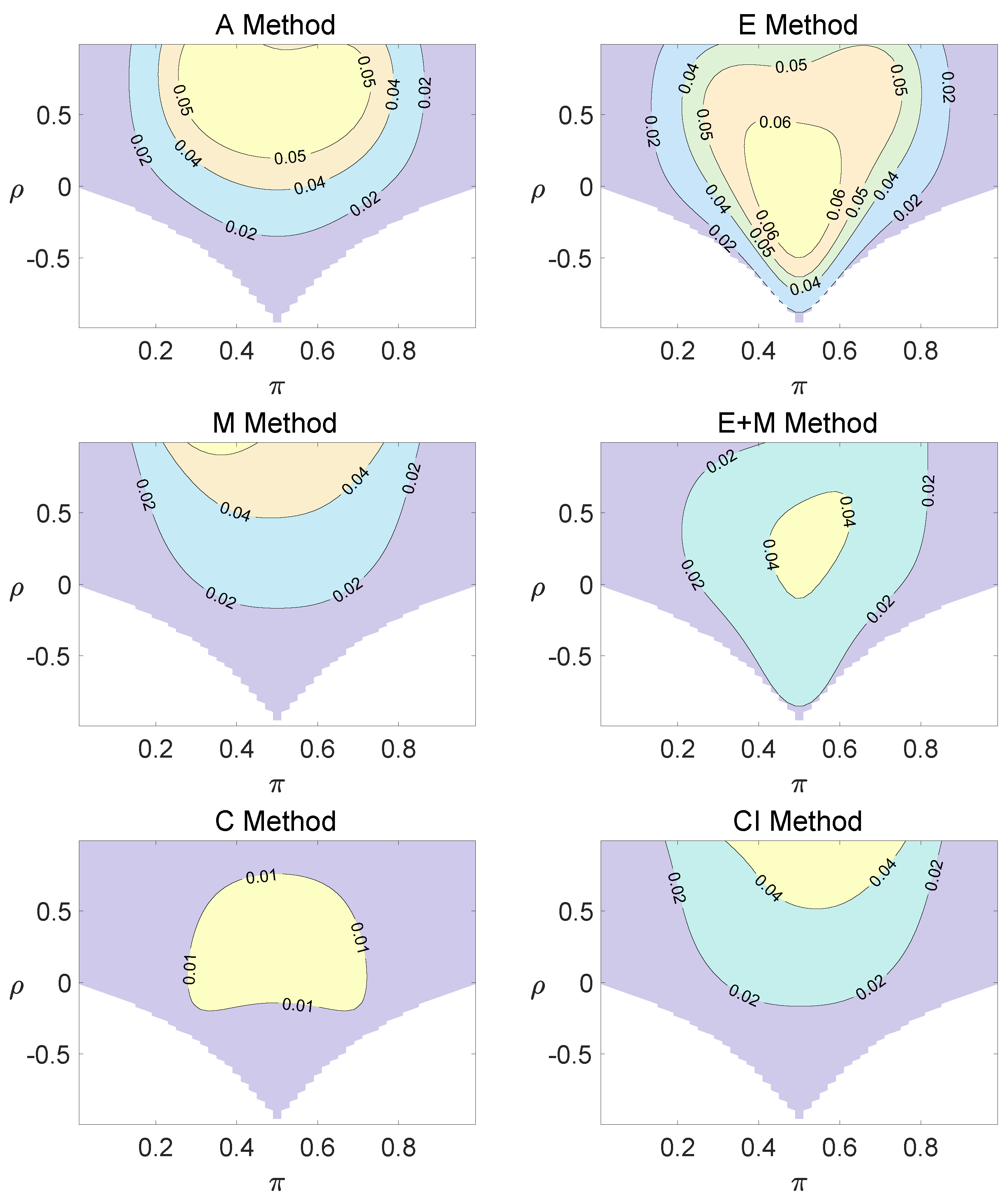
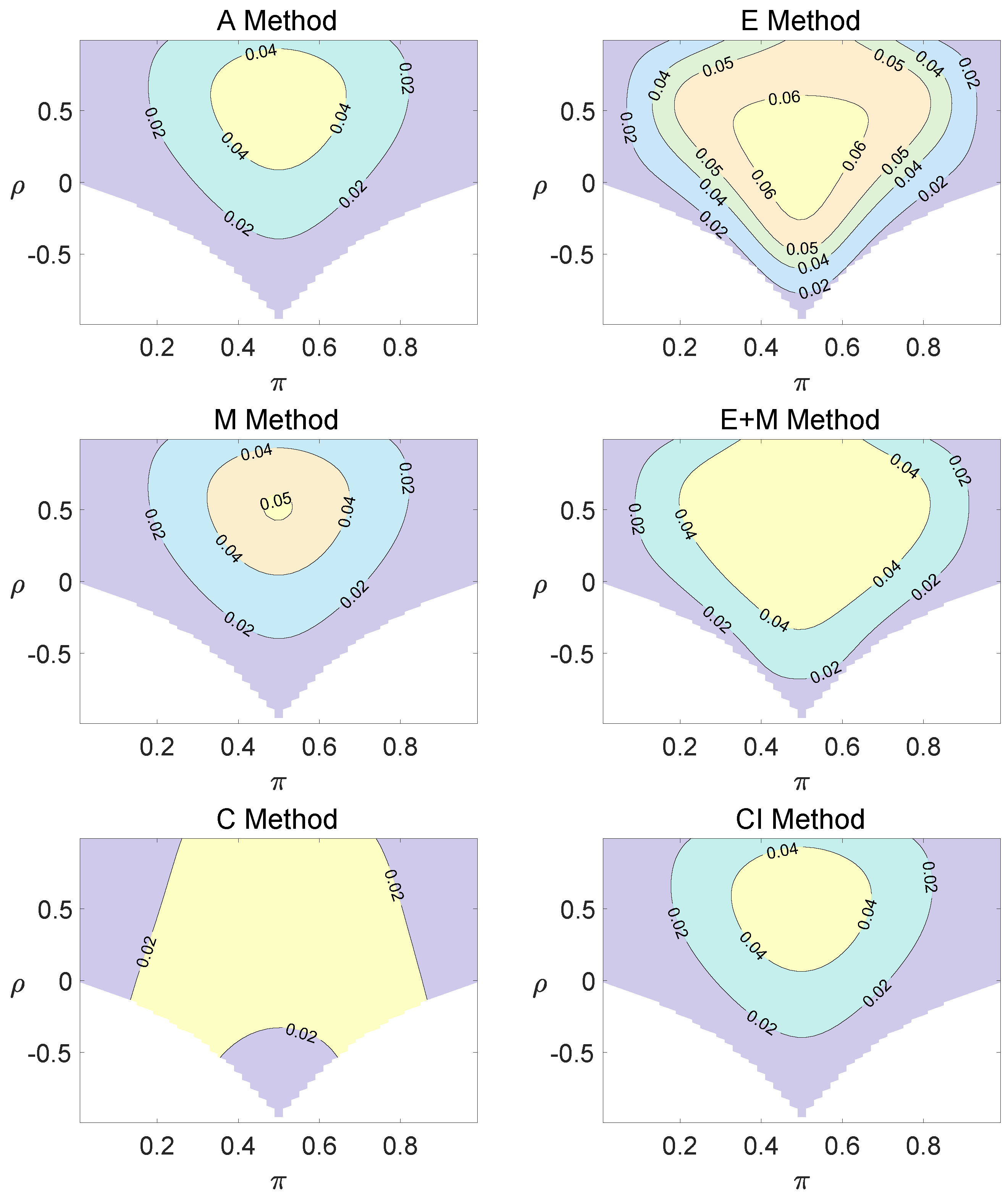
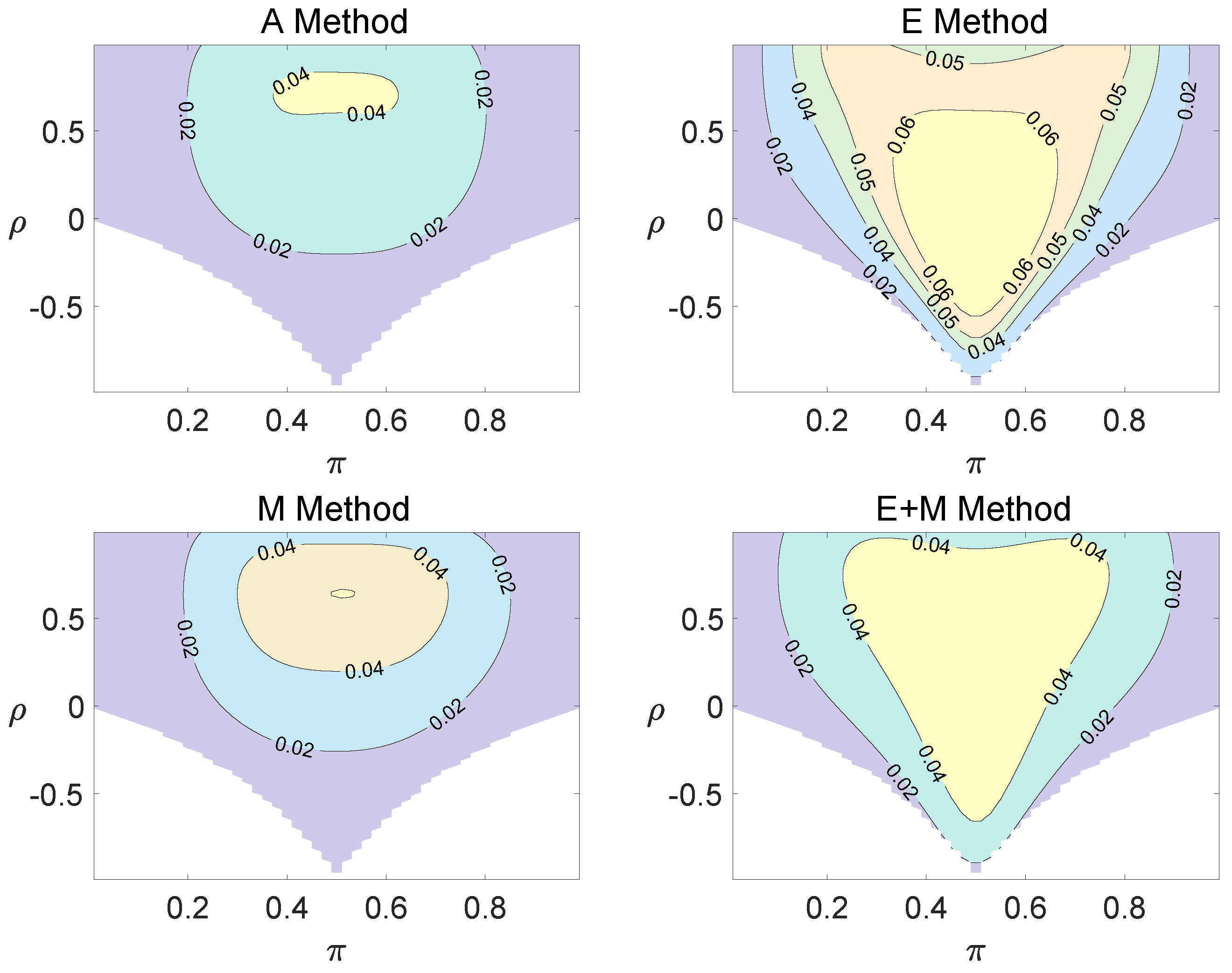
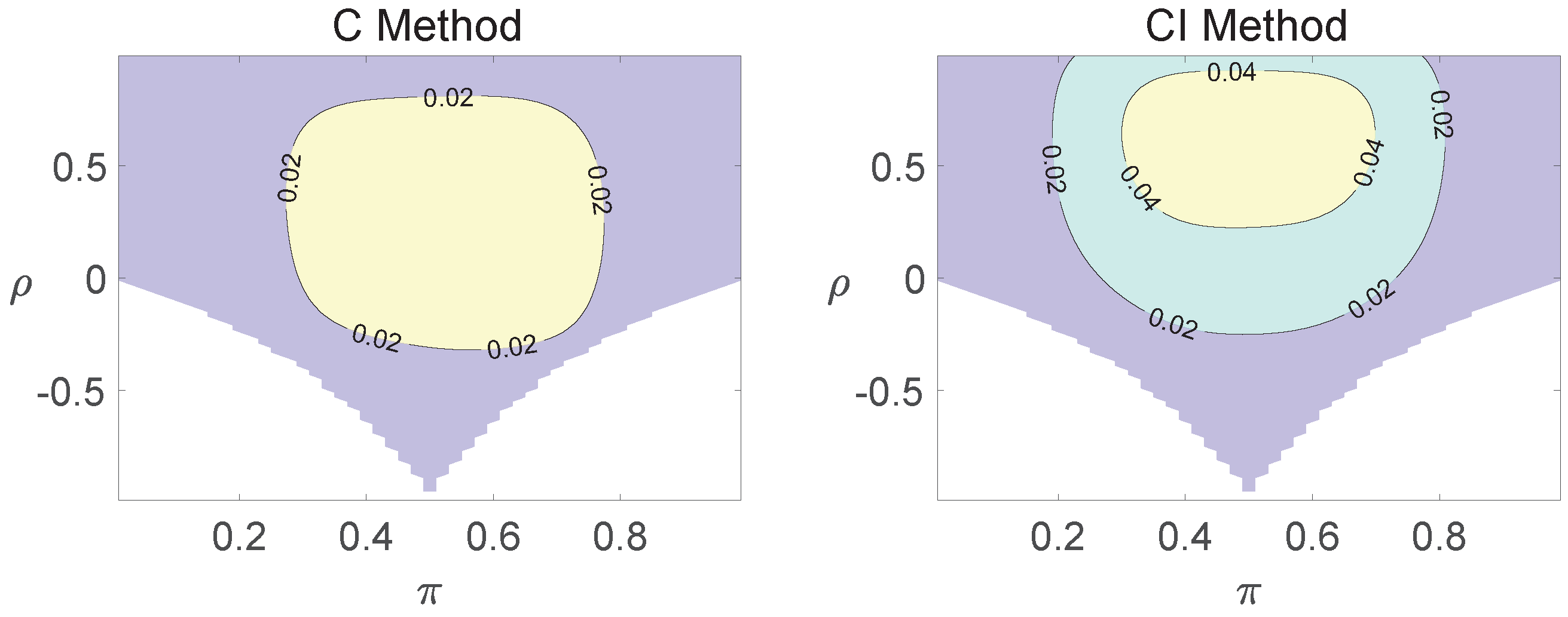
For the equal correlation coefficients model, all tables having a given margin were enumerated, and the corresponding p-values based on the six methods discussed can be calculated. The type I errors and powers of each proposed method were determined by the summation of probabilities of tables with a p-value for and , respectively. We set the parameter in the CI method. Figure 1, Figure 2 and Figure 3 demonstrate the contour plots of type I error rates as a function of and when the total sample size is around 10. The contour plots of type I error rates given a sample size of approximately 20 are shown in Figure A1 and Figure A2. The blank areas in the plots represent combinations of and for which at least one of the parameters () falls outside the interval [0, 1]. If the type I error of a test is greater than 6%, the test is considered liberal. And if the type I error of a test is less than 4%, the test is considered conservative according to Tang et al. [18].
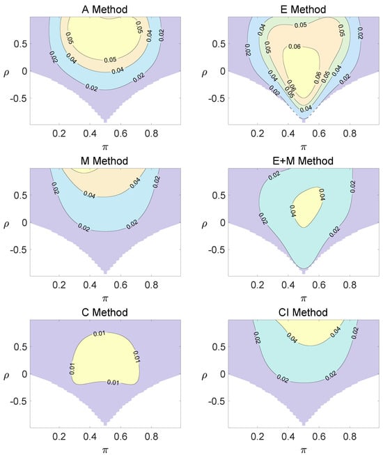
Figure 1.
Contour plots of type I errors for the equal correlation coefficients model (, , , ).
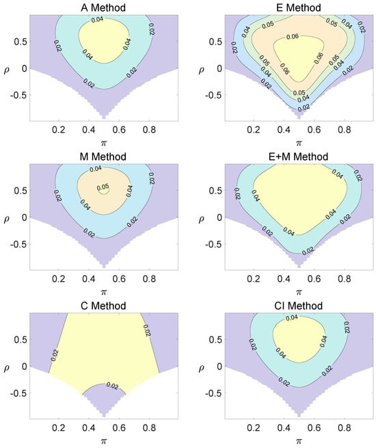
Figure 2.
Contour plots of type I errors for the equal correlation coefficients model (, , , ).
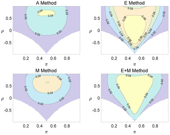

Figure 3.
Contour plots of type I errors for the equal correlation coefficients model (, , , ).
Regardless of the sample size and the group number, the asymptotic method, the M method, the E + M method, the C method, and the CI method typically yield conservative type I errors since a large area of combinations of and producing TIEs ≤ 0.04 is observed. The CI approach and the M approach generate very similar results due to their similar constructions of p-values. The CI approach defines the p-values within the space consisting of two confidence intervals, and the M approach considers the whole parameter space. When the total sample size is around 10, the C method produces extremely conservative outcomes with all parameter settings generating TIEs that are less than 3% due to discreteness. Although the E method generates a small proportion of area in the contour plots where the type I errors exceed 6%, it maintains a larger portion of type I error rates within the range of 4% and 6% compared to the other five methods.
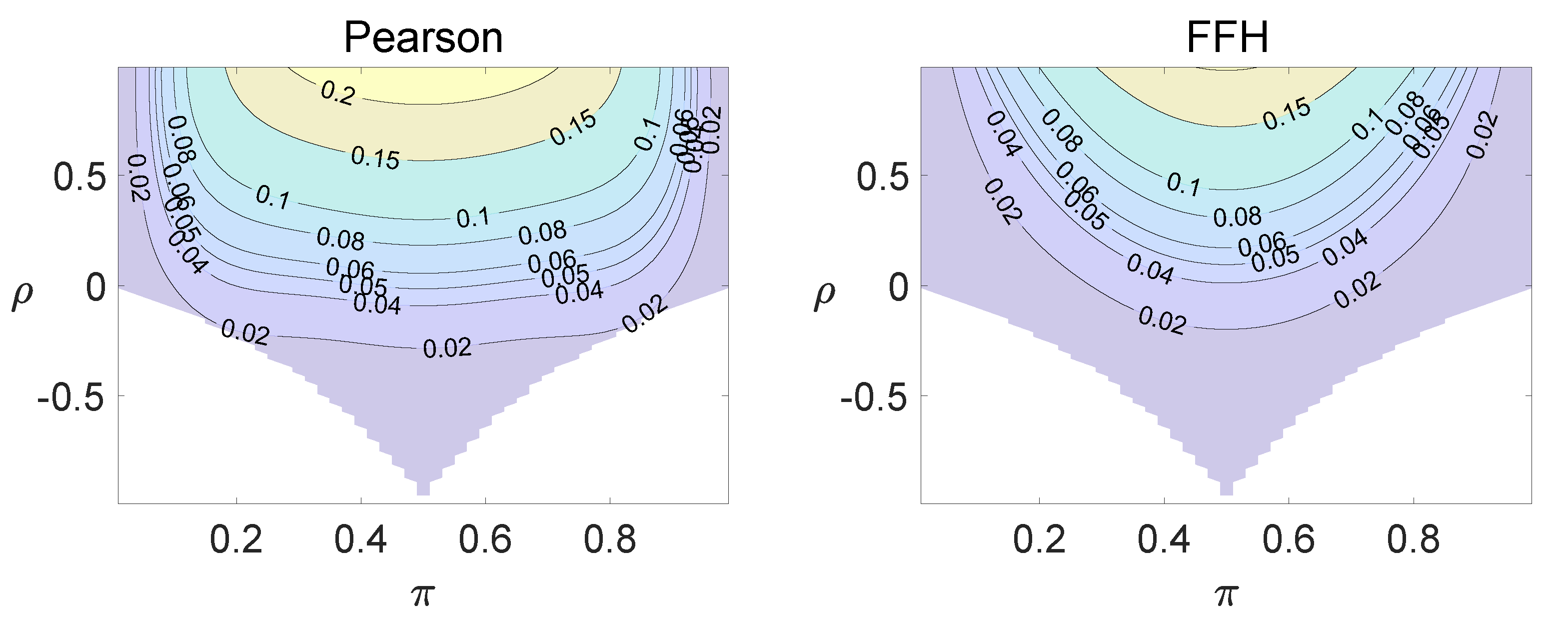
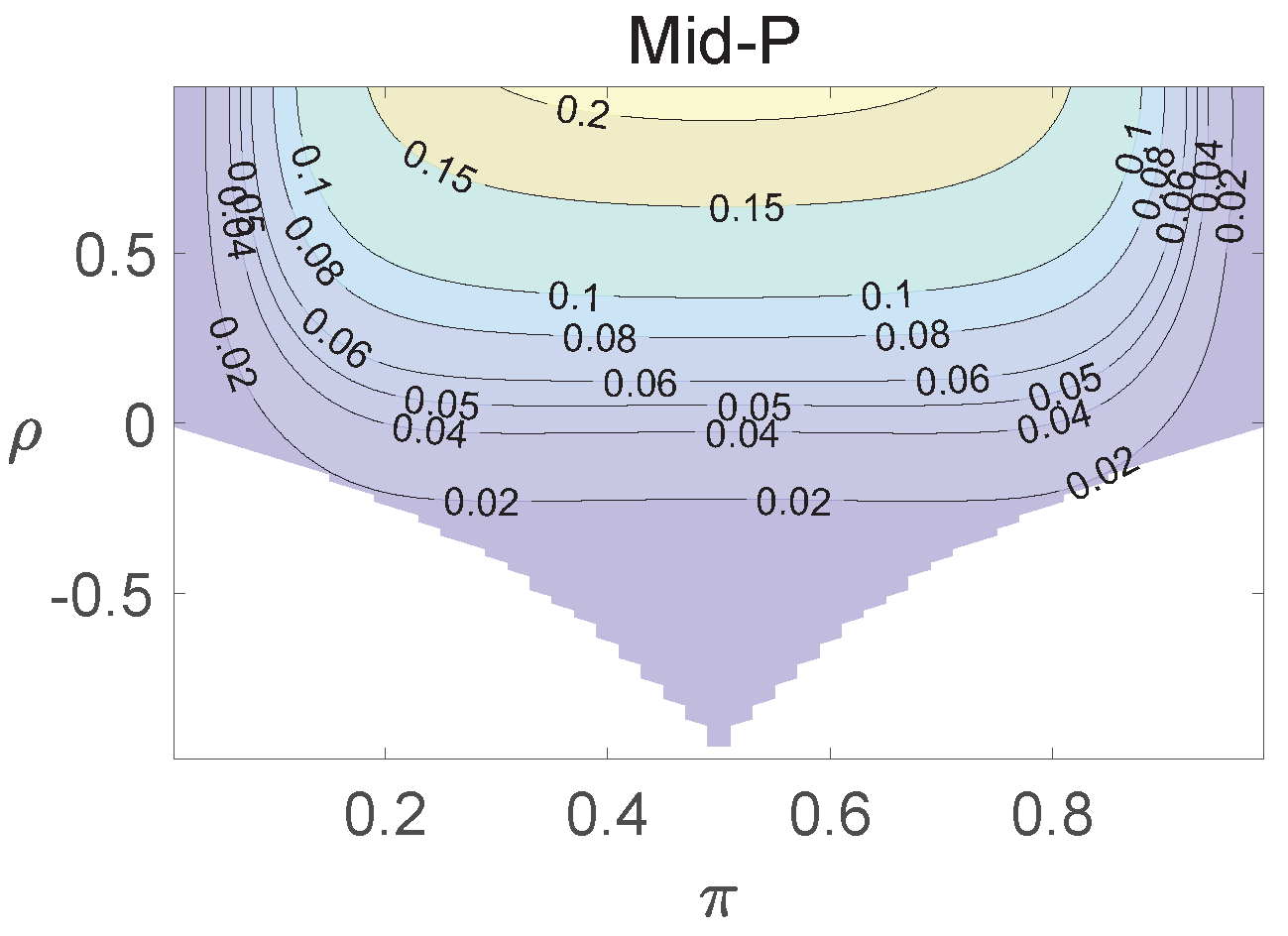
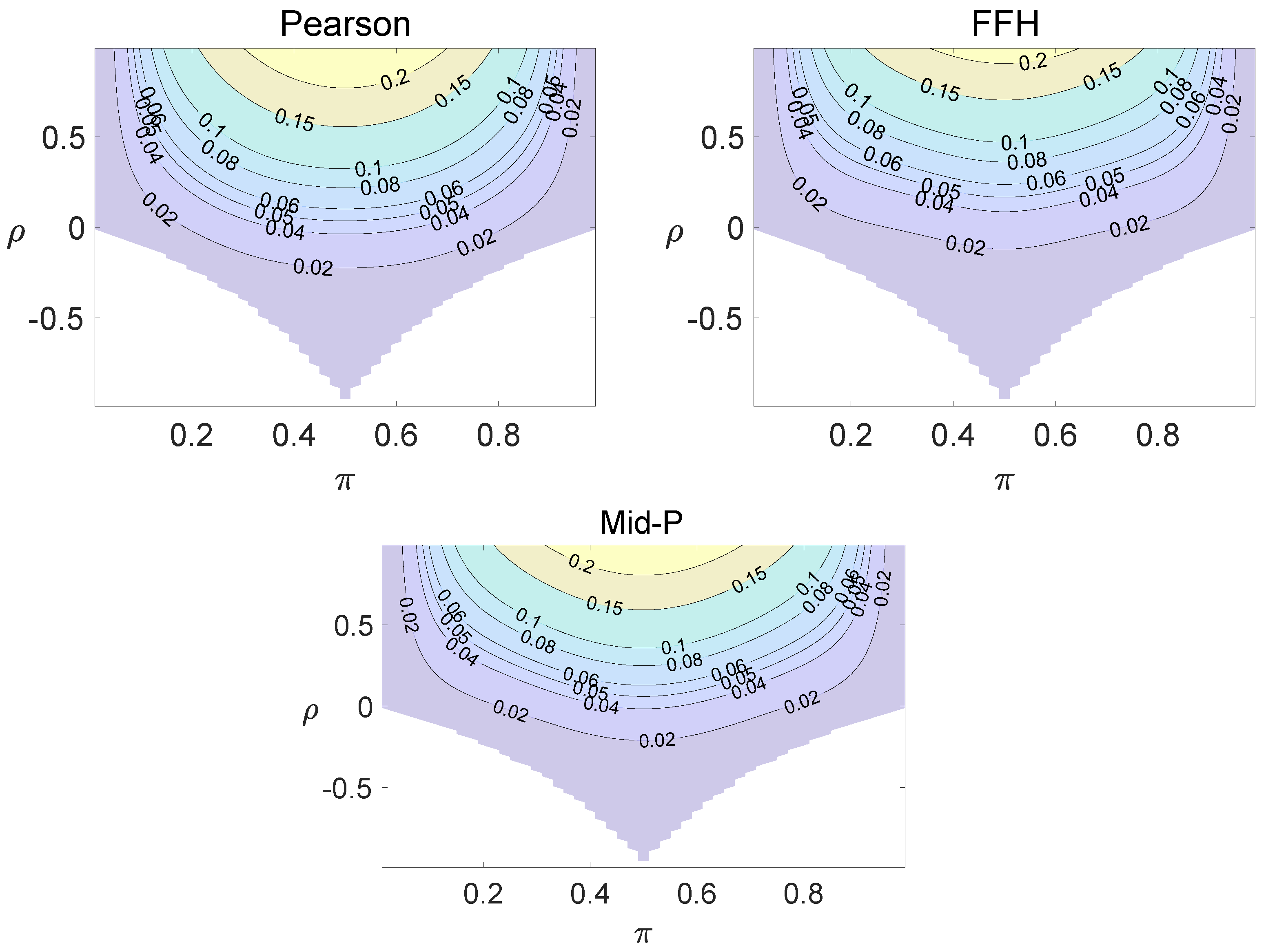
For each combination of from Figure 1, Figure 2 and Figure 3 and from Figure A1 and Figure A2, a parallel study was conducted using the individual site model. For example, tables with and can be transformed to , where . The performance of type I error controls of the Pearson chi-squared test, the FFH test, and the mid-P test were investigated, and the contour plots are exhibited in Figure 4, Figure 5 and Figure 6 and Figure A3 and Figure A4.
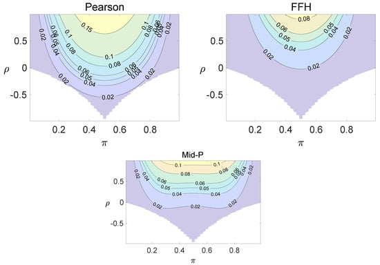
Figure 4.
Contour plots of type I errors for the individual site model (, , , ).

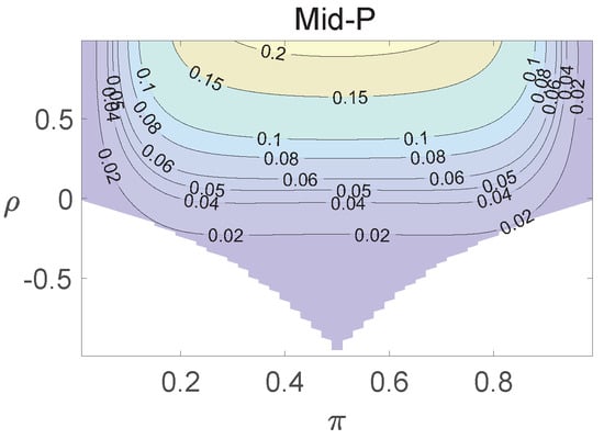
Figure 5.
Contour plots of type I errors for the individual site model (, , , ).
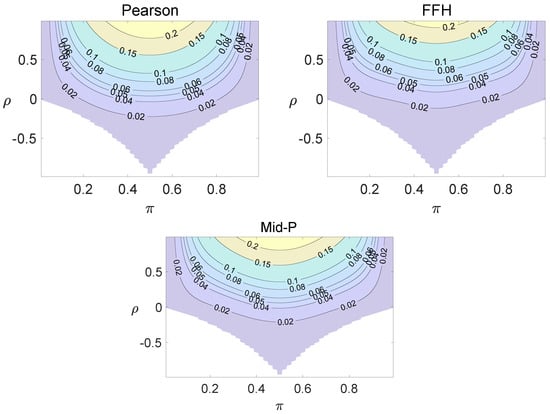
Figure 6.
Contour plots of type I errors for the individual site model (, , , 1, 2, 3.4).
Using the individual site model, the Pearson, the FFH, and the mid-P test generate inflated type I errors when the underlying correlation coefficient is close to 1, while the FFH approach outputs conservative TIEs when . If the two sites of a subject have a weak correlation (), type I errors from the three methods can be controlled within the satisfied region. Hence, the equal correlation coefficients model is recommended in practice given the unsatisfied type I error controls when the correlation is ignored.
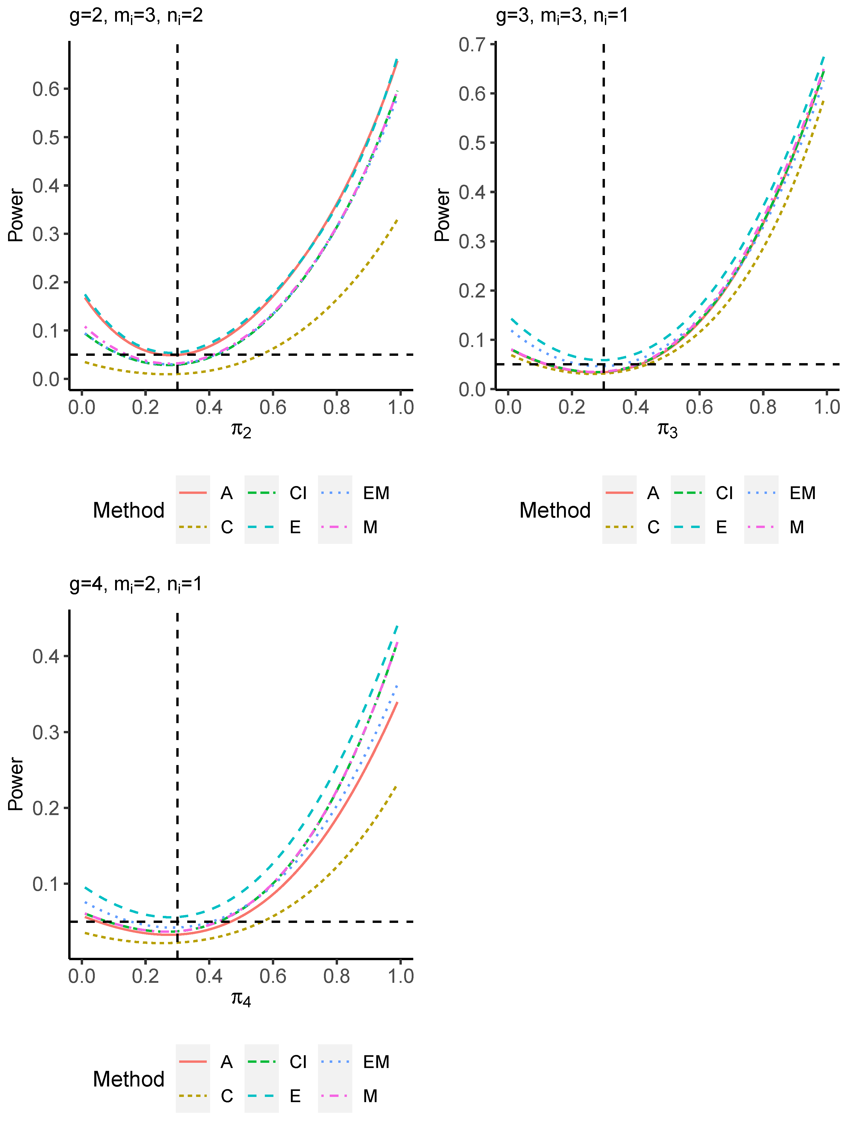
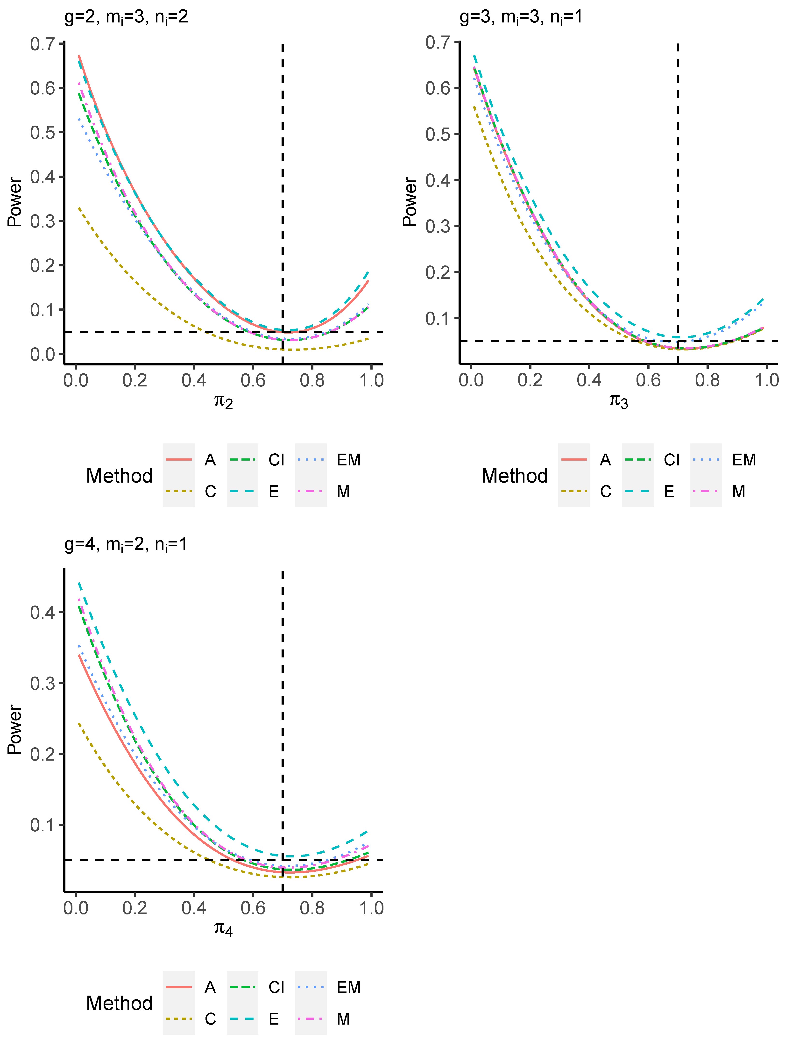
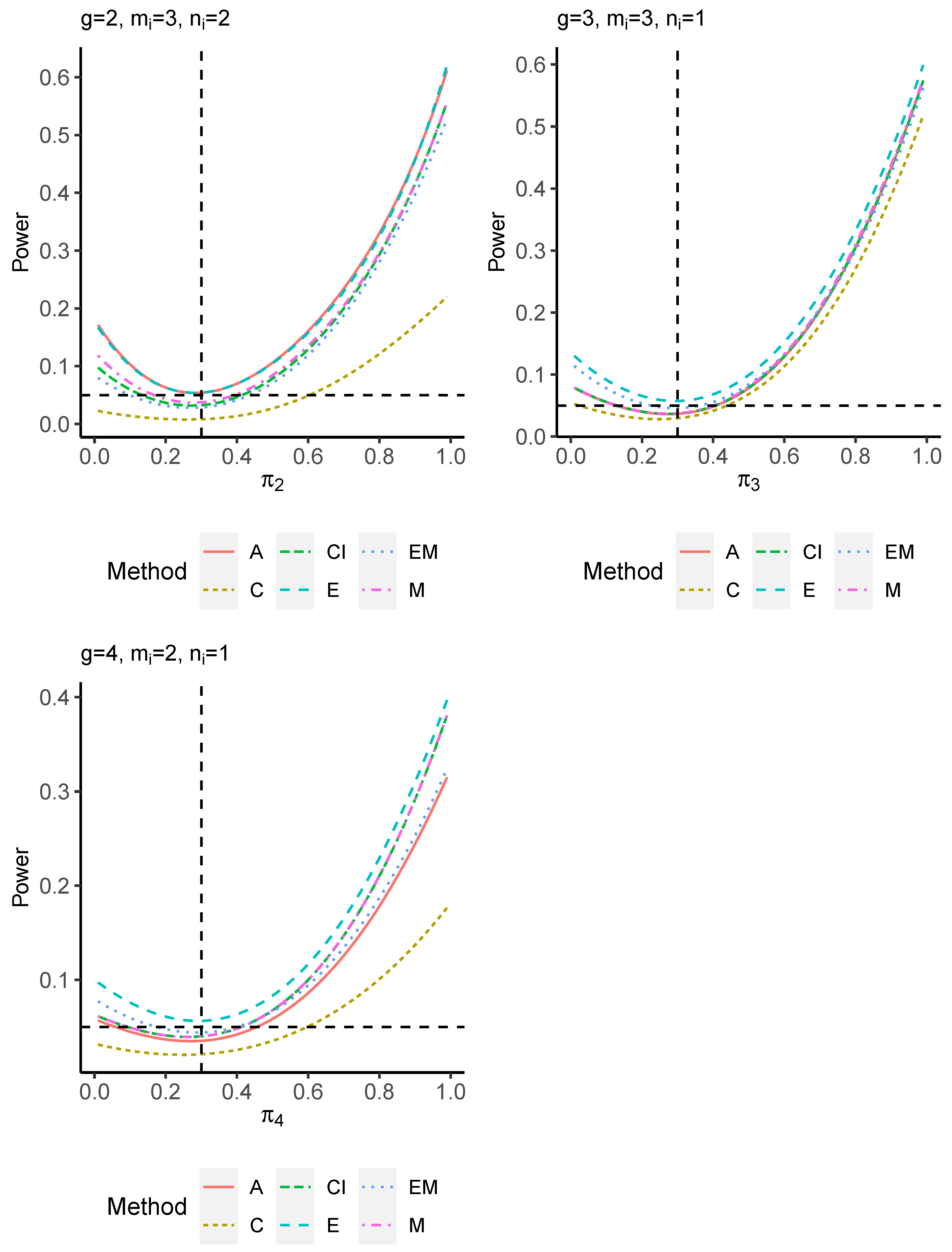
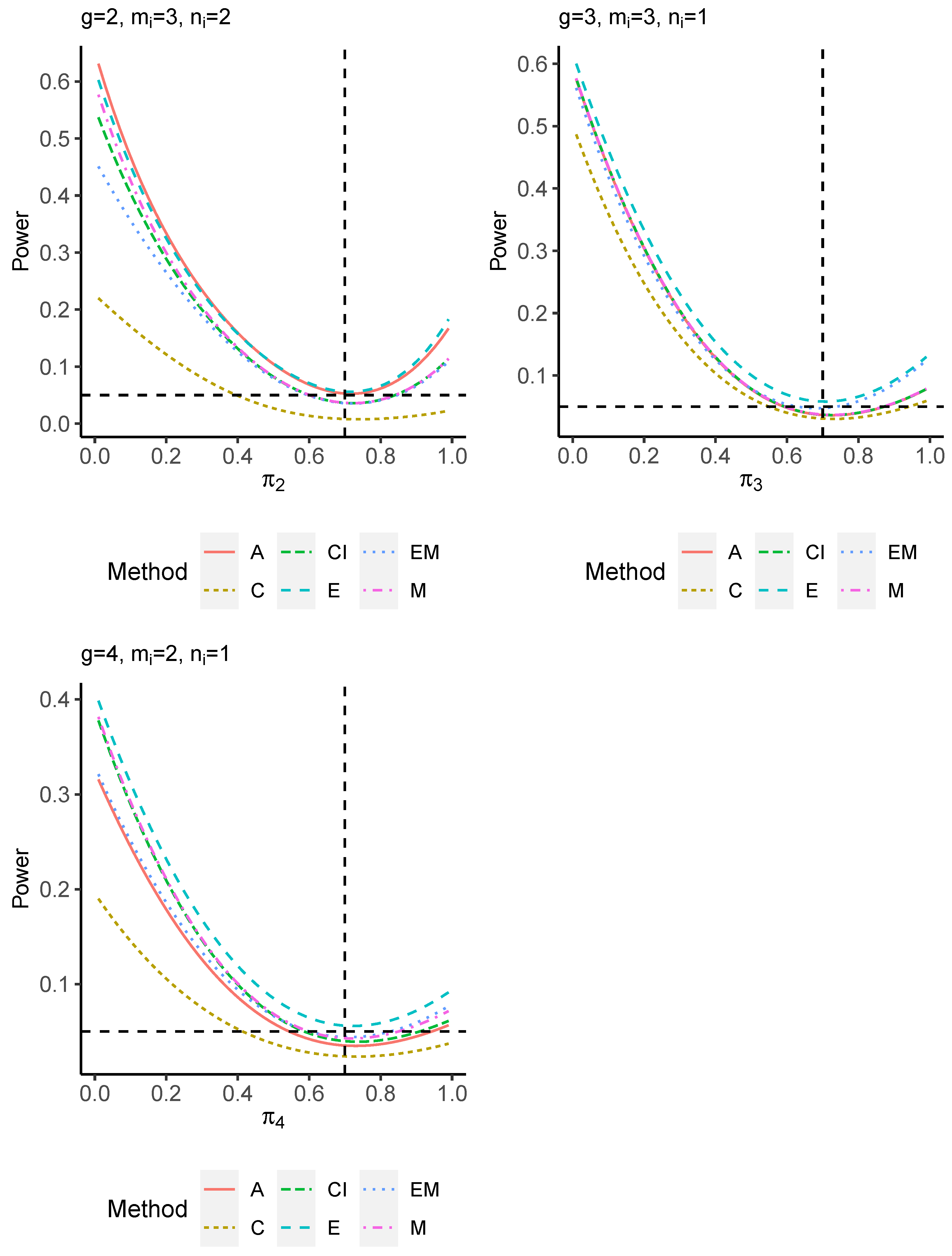
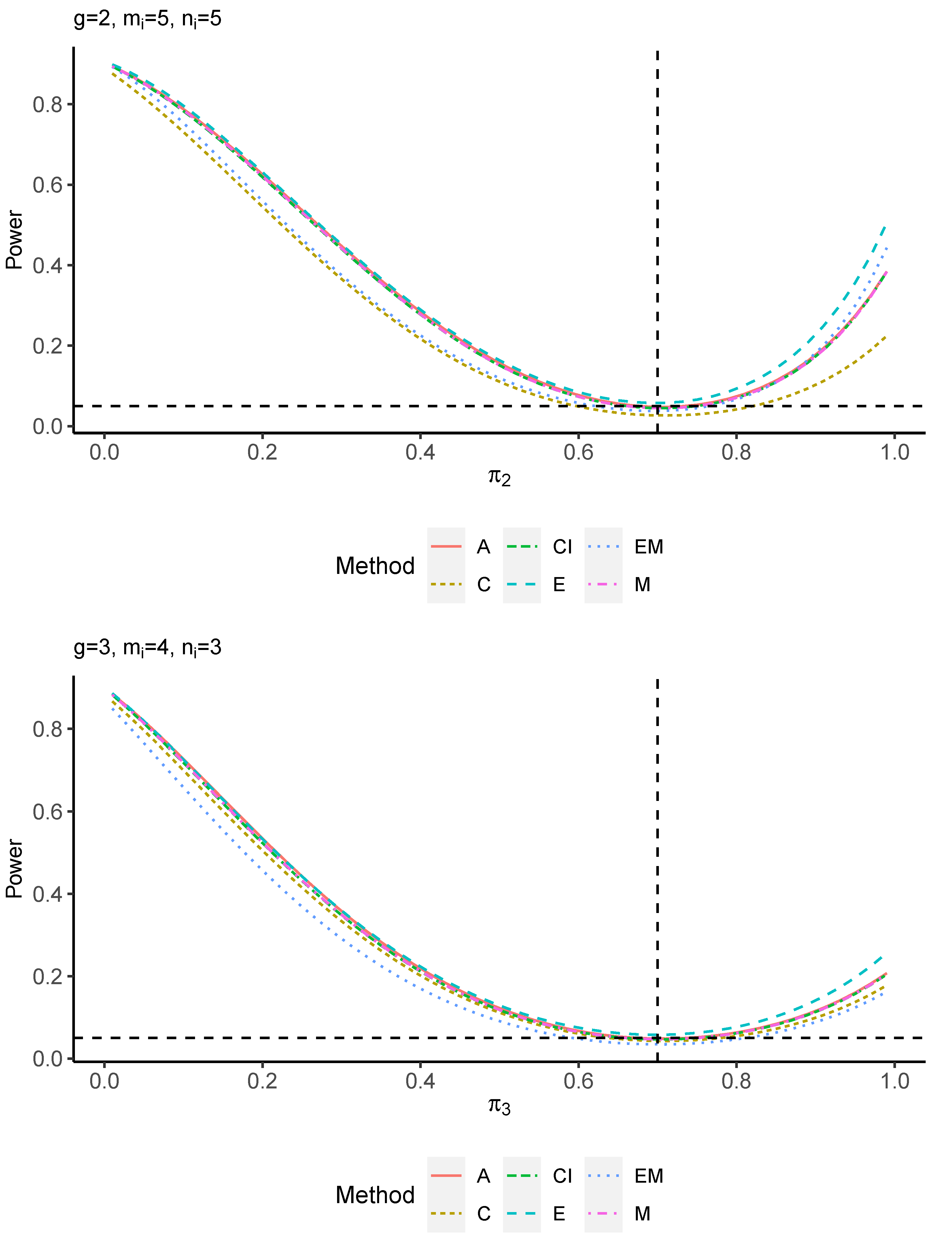
The power performance is investigated in the following part. The exact power is determined by varying the value of while fixing , and . Based on Figure 7, Figure 8, Figure 9 and Figure 10 and Figure A5, Figure A6, Figure A7 and Figure A8, the E method outperforms the other five methods and have the highest powers in all scenarios. The power of the C approach is generally the lowest, which is expected given the low type I error rates observed in the numerical study above. Again, the CI and the M method generate very similar powers due to the intrinsic similarities. Note that if the absolute difference between and the value of decrease to 0, the powers of all methods become close to 0.05 as indicated by the horizontal dash lines. This behavior is anticipated because the smaller the difference, the more likely the tables will support the null hypothesis. The statistical test powers increase as the sample size increases from 10 to 20 no matter what method is employed.
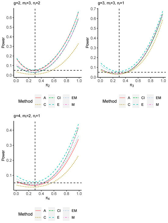
Figure 7.
Power plots for , and .
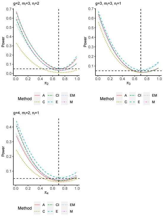
Figure 8.
Power plots for , and .
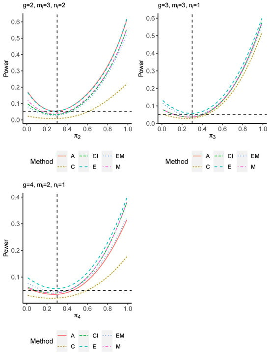
Figure 9.
Power plots for , and .
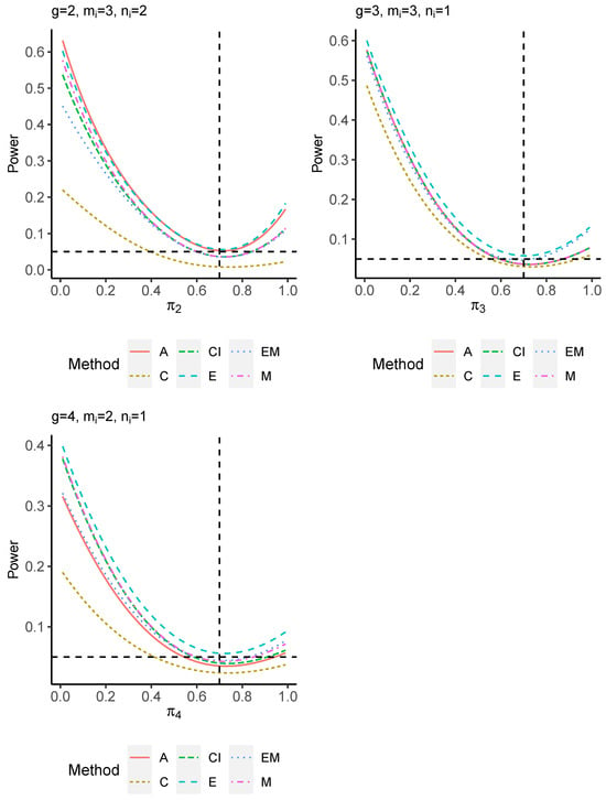
Figure 10.
Power plots for , and .
7. Real Examples
Three real-world examples are described in detail to demonstrate the application of the proposed methods. The first example is a double-blind randomized clinical trial studying acute otitis media with effusion (OME) as described by Mandel [19]. The total number of children recruited in the study was 214, and there were two hundred and ninety-three ears registered in the study among these children. Every participant was categorized into either the bilateral disease or unilateral disease group at the study entry. All subjects underwent either unilateral or bilateral tympanocentesis and were subsequently randomized into one of two treatment groups, cefaclor or amoxicillin, for 14 days. After the course of treatment, the disease status of each ear was recorded, and 11 children were dropped from the study since they met the exclusion criteria. Table 3 displays the distribution of a subgroup of children aged ≥ 6 years. To test the homogeneity of cure rates of the two treatments, the six methods discussed in Section 5 were applied, and the corresponding p-values can be found in Table 4. All p-values are greater than 0.05, suggesting a lack of evidence to reject the null hypothesis at .

Table 3.
The distribution of children aged ≥ 6 years at 14 days by treatment, number of cured ears, and disease status at study entry.

Table 4.
p-values using different approaches for example 1.
The second example consists of 60 subjects receiving Orthokeratology (Ortho-k) to treat nearsightedness. This is an observational study conducted at the First Affiliated Hospital of Xiamen University in 2023 (Liang et al. [20]). Ortho-k is a vision correction procedure that uses specially designed contact lenses to temporarily reshape the cornea and improve vision. The study involved various brands that can be further classified into two categories based on the type of lens designs. Vision shaping treatment (VST) is one of the two designs constructing the edge of the lens that touches the edge of the cornea, while the other design, called corneal refractive therapy (CRT), constructs the edge of the lens so that it does not touch the cornea (Lu et al. [21]). Patients can opt to wear the lenses on either one or both eyes, depending on their individual requirements. An eye is said to have a response to the treatment if the axial length growth mm according to Rose et al. [22]. A subgroup of female subjects were included in the demonstration to test whether there was a difference between the response rates of the two designs. There were 3 subjects who received unilateral Ortho-k and 26 subjects who underwent bilateral Ortho-k, as indicated in Table 5. The p-values from Table 6 are all less than the nominal level of 5%, suggesting a rejection of the null hypothesis.

Table 5.
The number of subjects by design and number of eyes demonstrating response after treatment.

Table 6.
p-values using different approaches for example 2.
The data of the third example were collected from patients with retinitis pigmentosa referred from the outpatient facilities of the Massachusetts Eye and Ear Infirmary or from private ophthalmologists. Details of the study can be found in Berson, Rosner, and Simonoff [23]. The patients were classified into four groups based on their genetic types, which are autosomal dominant RP (DOM), autosomal recessive RP (AR), sex-linked RP (SL), and isolate RP (ISO). The type ISO was dropped from the analysis since the sample size of this group is large and asymptotic methods are preferred. The distribution of patients can be found in Table 7. This example demonstrates the capability of the proposed methods in handling bilateral data. The calculation time of the E + M method is excessively long; therefore, the corresponding p-value is omitted. All the p-values of the proposed methods displayed in Table 8 are less than 0.05, indicating a rejection of the null hypothesis, and the prevalences of the three groups are not the same.

Table 7.
The number of patients by genetic type and number of affected eyes.

Table 8.
p-values using different approaches for example 3.
8. Discussion
The individual site model assumes the measurements from sites of individuals are independent and does not consider the potential correlation between two sites of the same subject. Given prior knowledge of the nonexistence of the correlation, an investigator may choose to proceed with the individual site model and perform the Pearson chi-squared test or exact tests without doubt. However, it is often the case that there is no proven fact of such an assumption. As the correlation moves further from zero, the asymptotic and exact methods lose the type I error controls based on the numerical studies in Section 6. One may argue that the individual site model may carry out the hypothesis test using an appropriate method with acceptable TIEs falling in the interval of . It is important to note that the equal correlation coefficients model also produces satisfactory TIE controls with a suitable approach. Therefore, the model taking into account the correlation takes precedence if the data collection involves paired sites of the same subject.
Given the priority of the equal correlation coefficients model, testing the homogeneity of group-specific proportions using the score test can be the first candidate method that researchers consider. Nevertheless, the asymptotic behavior of the score test is not guaranteed if the sample size is small. As a consequence, five exact tests are proposed, and their performance in terms of TIE controls and statistical powers was examined in different scenarios. When the sample size is relatively small as seen in Figure 1, Figure 2 and Figure 3, the E method generally performs well in controlling TIEs within 4% to 6%, while other methods are conservative with larger proportions in the contour plots below 4%. This superiority of the E method can be found in Figure A1 and Figure A2 where the sample size is relatively large. Regarding statistical powers, the E method is superior or similar to other methods for all sample sizes and parameter settings. For example, the E method has similar powers to the asymptotic method when and differentiates from other methods when or 4 in Figure 7. Overall, the E method is recommended as it controls type I error in a satisfactory region and has higher powers than the other methods. The M, E + M, and CI methods generally produce comparable TIEs and powers, whereas the C method becomes the most conservative specifically when the total sample size is approximately 10. Future works will include validation of the equal correlation coefficient assumption before performing the homogeneity test.
9. Conclusions
There are two aims of this article: first, to investigate and compare the two models with and without the assumption of correlation coefficients, and second, to propose exact methods to address the lack of type I error controls caused by poor approximations of the score test when the sample size is small. The numerical study indicates the relative appropriateness of the equal correlation model when analyzing paired binary data and highlights the superiority of the E method for exact tests of homogeneity of proportions.
Author Contributions
All authors contribute equally to the manuscript. All authors have read and agreed to the published version of the manuscript.
Funding
This research received no external funding.
Data Availability Statement
Data are contained within the article.
Conflicts of Interest
The authors declare no conflicts of interest.
Appendix A
Let and be the true parameters with the null hypothesis and note that is uniformly distributed on [0, 1] with . Following the definition of , it is clear that
Appendix B
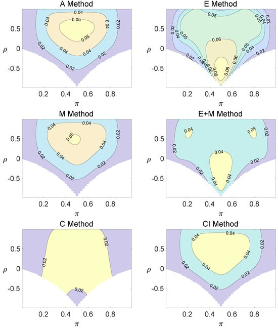
Figure A1.
Contour plots of type I errors for the equal correlation coefficients model (, , , ).
Figure A1.
Contour plots of type I errors for the equal correlation coefficients model (, , , ).
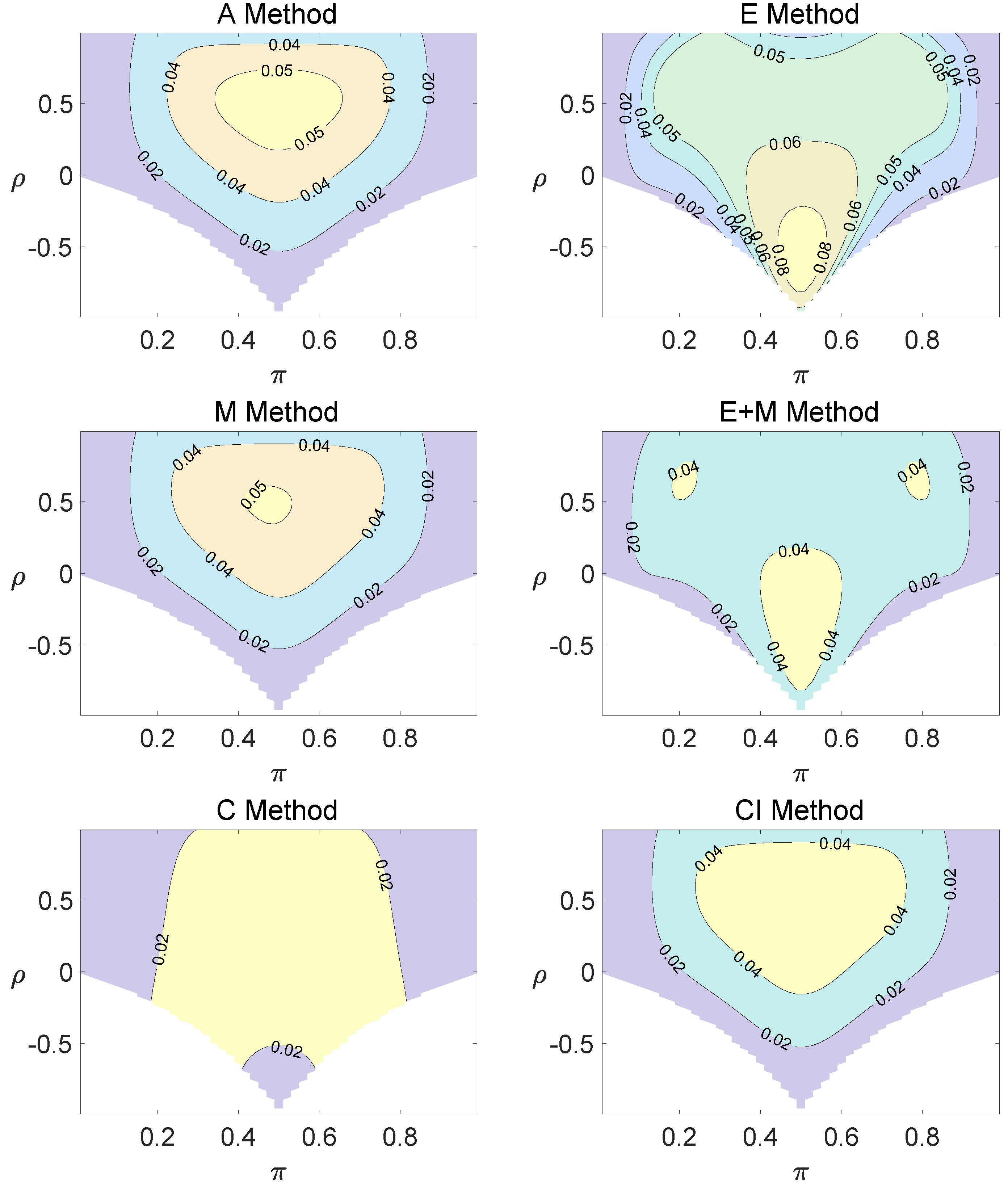
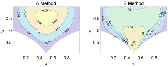
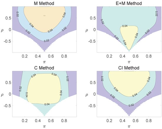
Figure A2.
Contour plots of type I errors for the equal correlation coefficients model (, , , ).
Figure A2.
Contour plots of type I errors for the equal correlation coefficients model (, , , ).
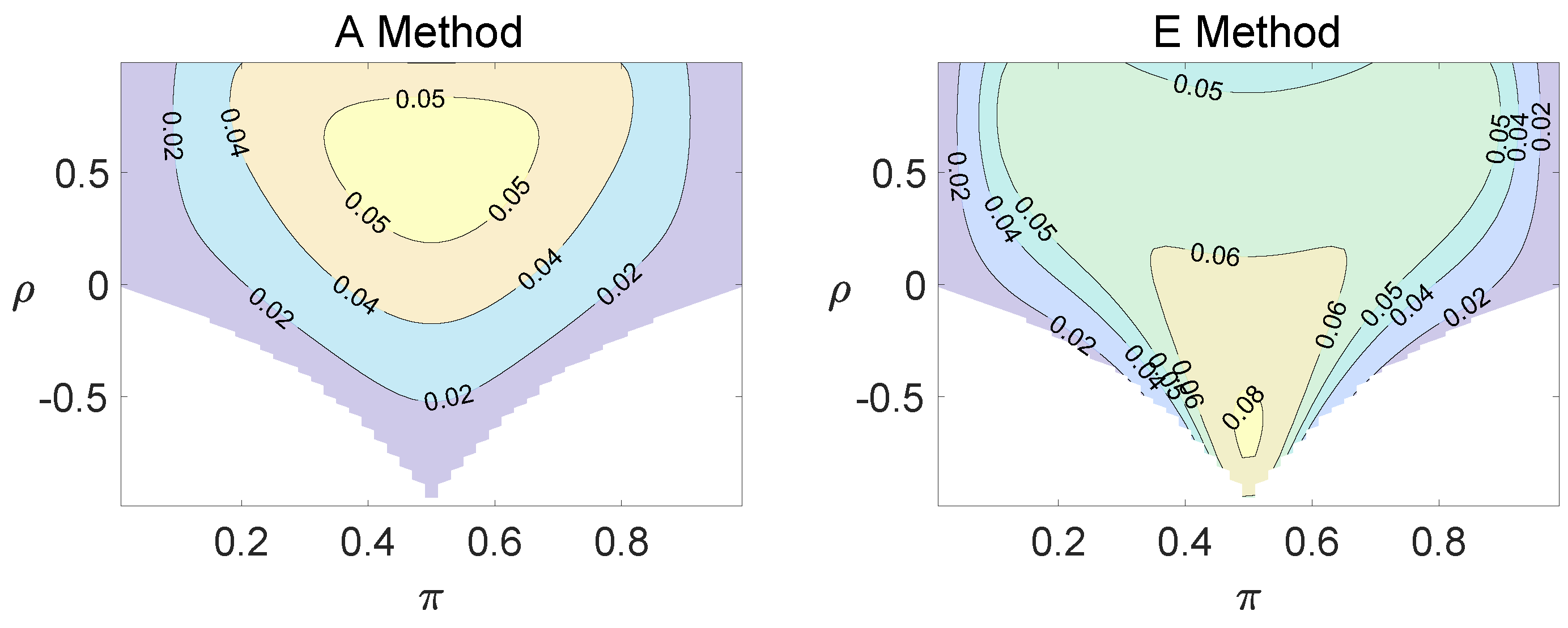
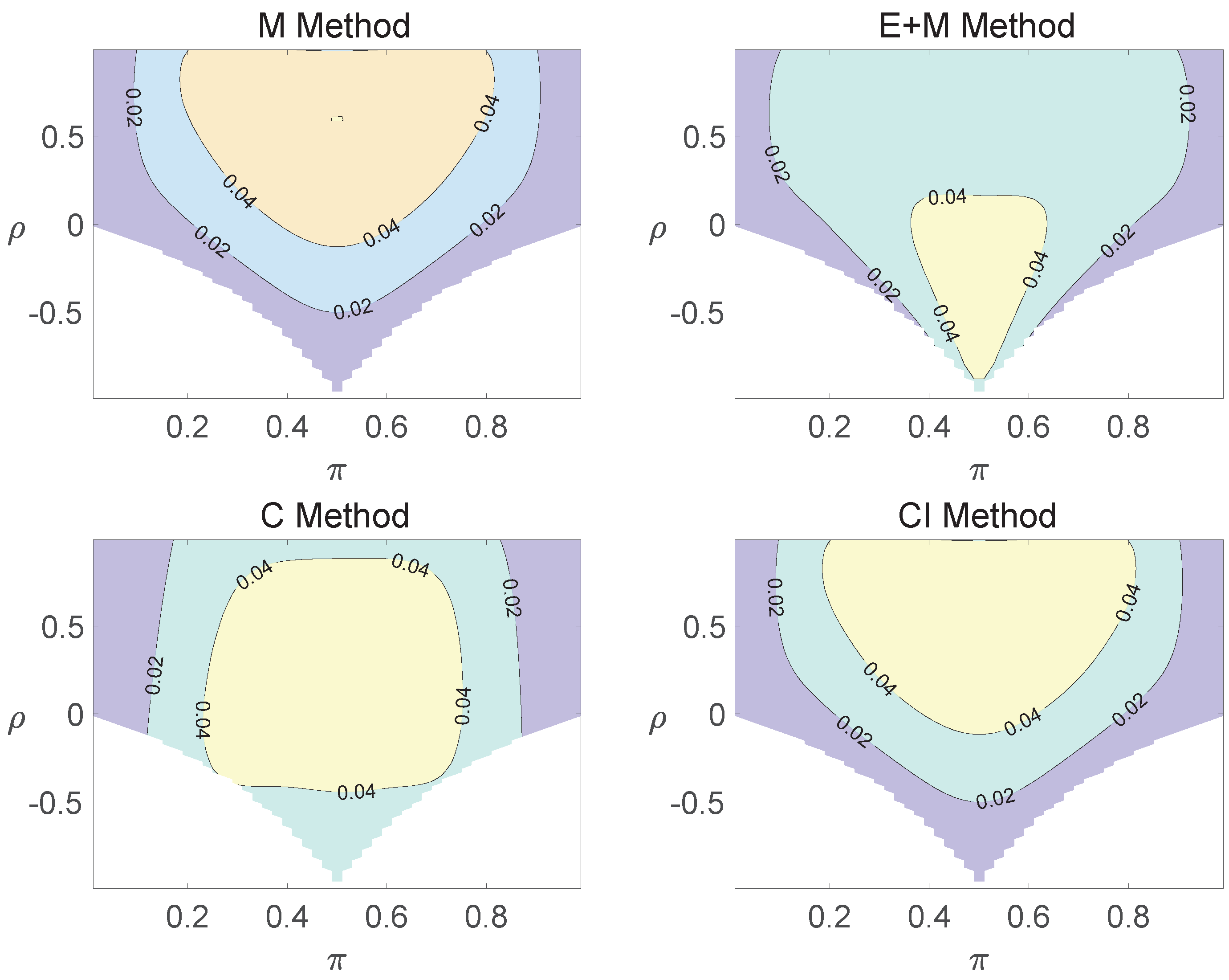
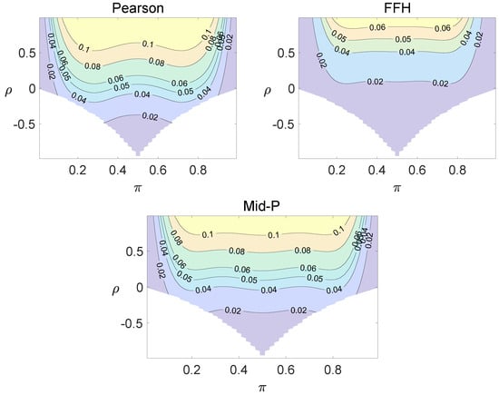
Figure A3.
Contour plots of type I errors for the individual site model (, , , ).
Figure A3.
Contour plots of type I errors for the individual site model (, , , ).
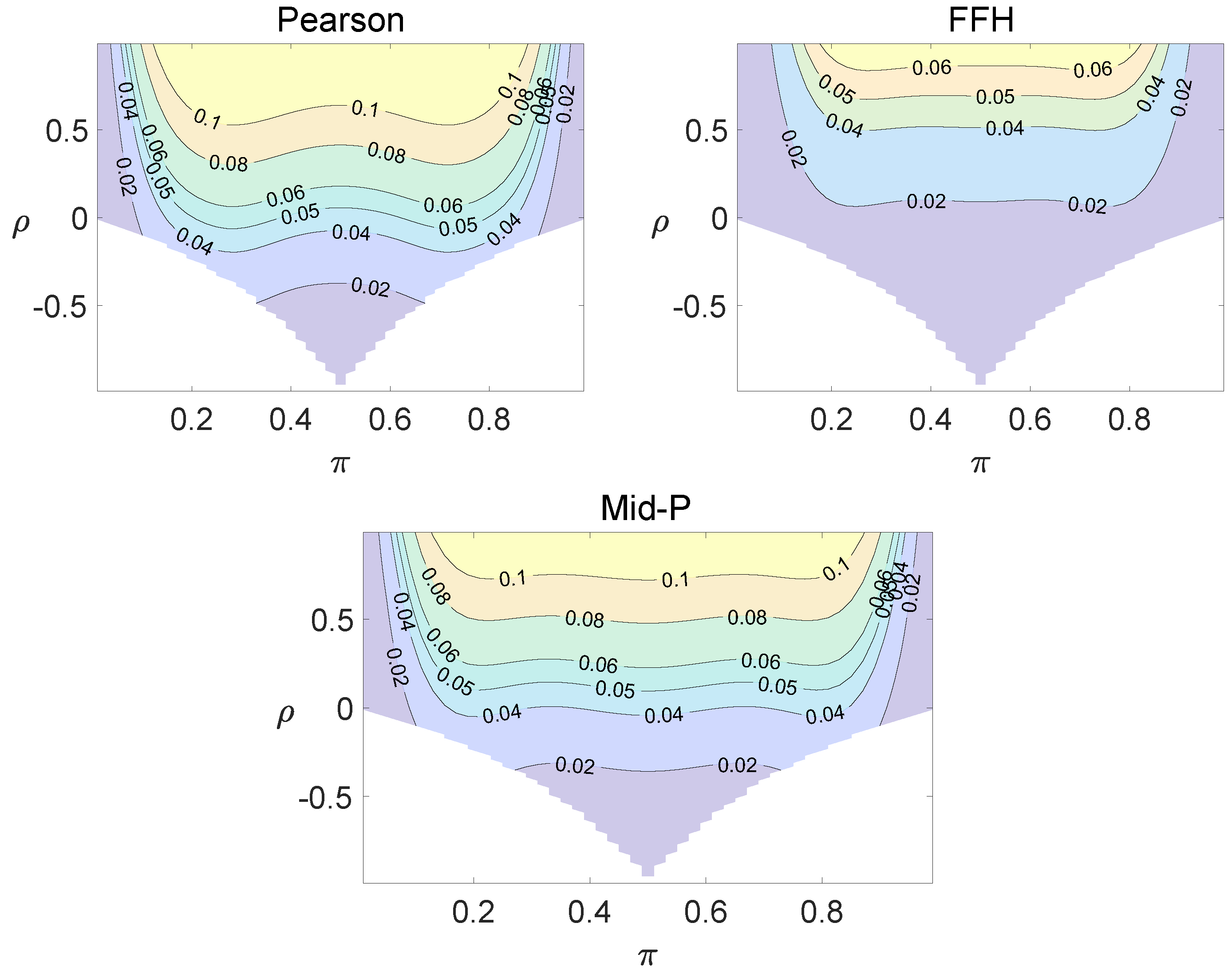
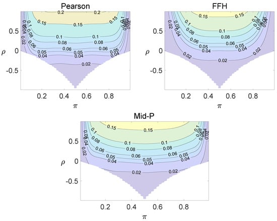
Figure A4.
Contour plots of type I errors for the individual site model (, , , ).
Figure A4.
Contour plots of type I errors for the individual site model (, , , ).

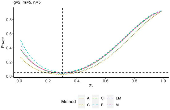
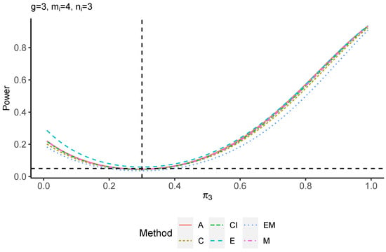
Figure A5.
Power plots for , and .
Figure A5.
Power plots for , and .
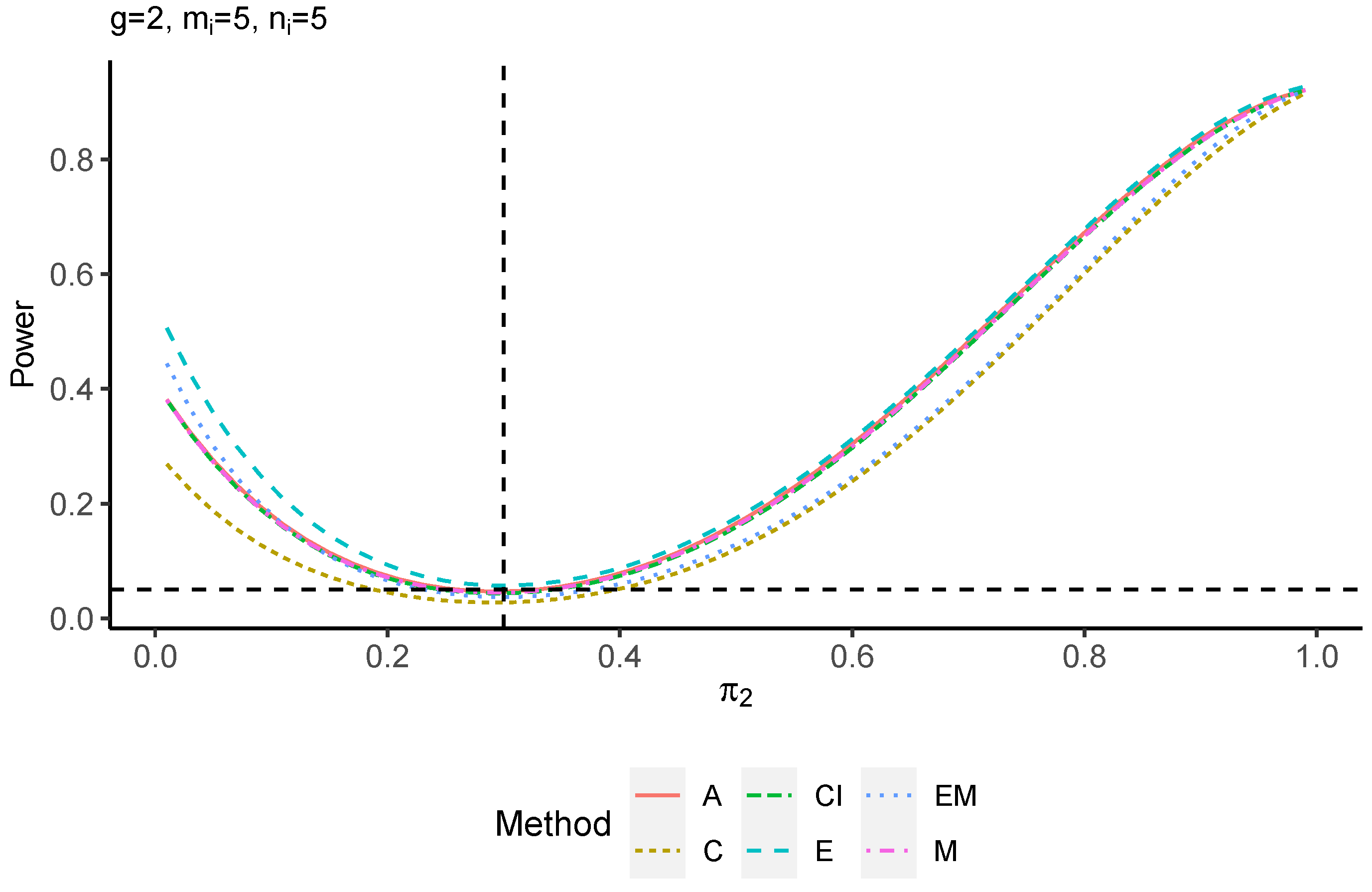
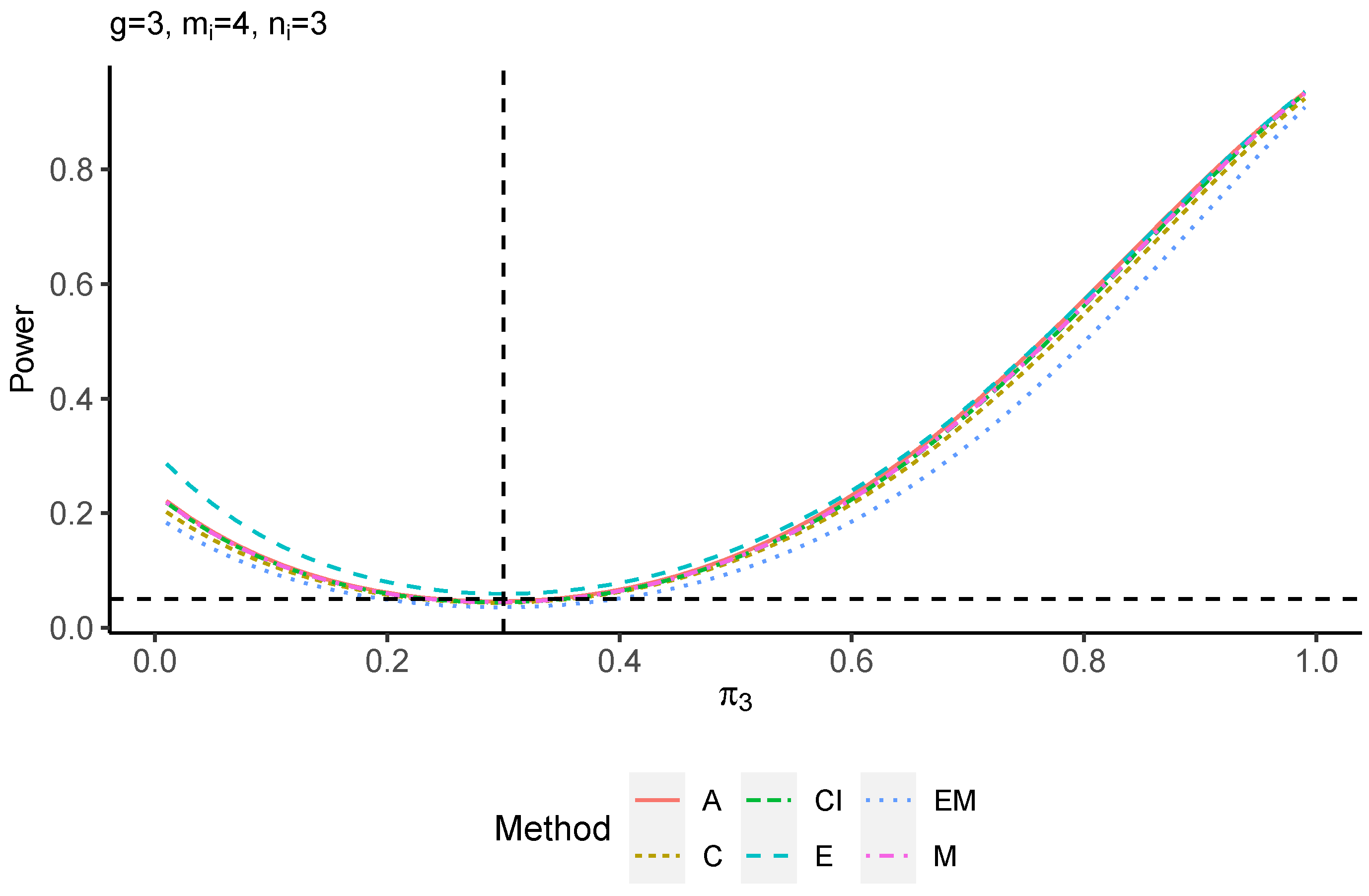
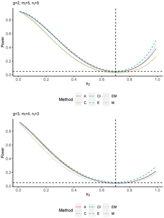
Figure A6.
Power plots for , and .
Figure A6.
Power plots for , and .
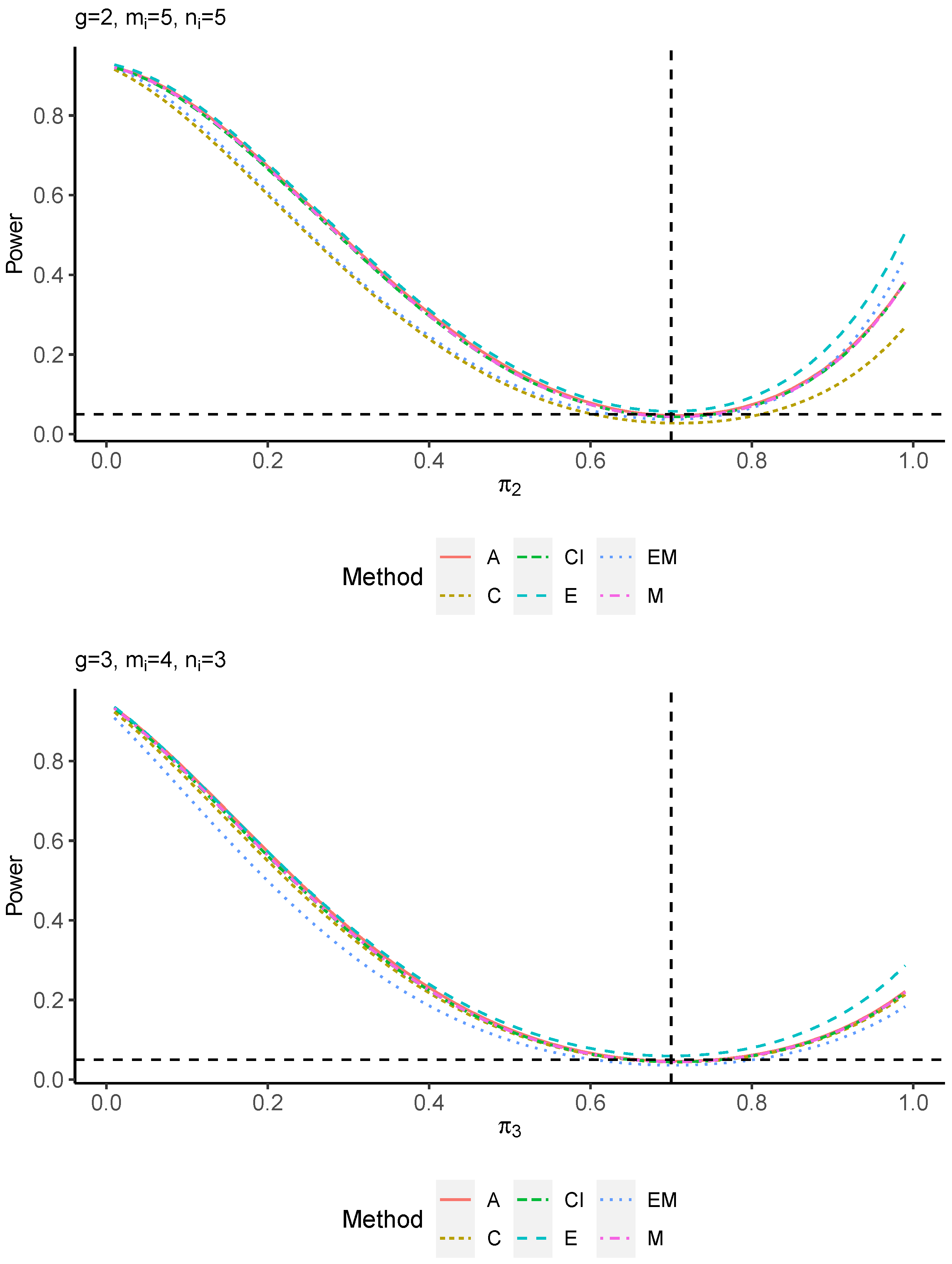
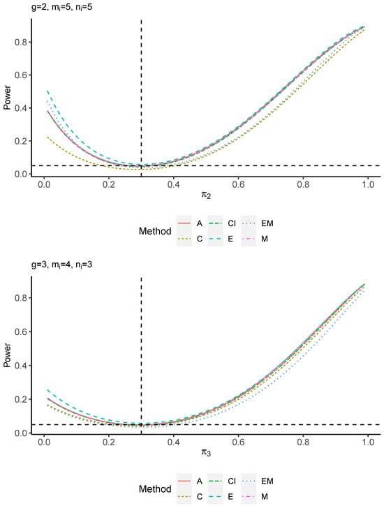
Figure A7.
Power plots for , and .
Figure A7.
Power plots for , and .
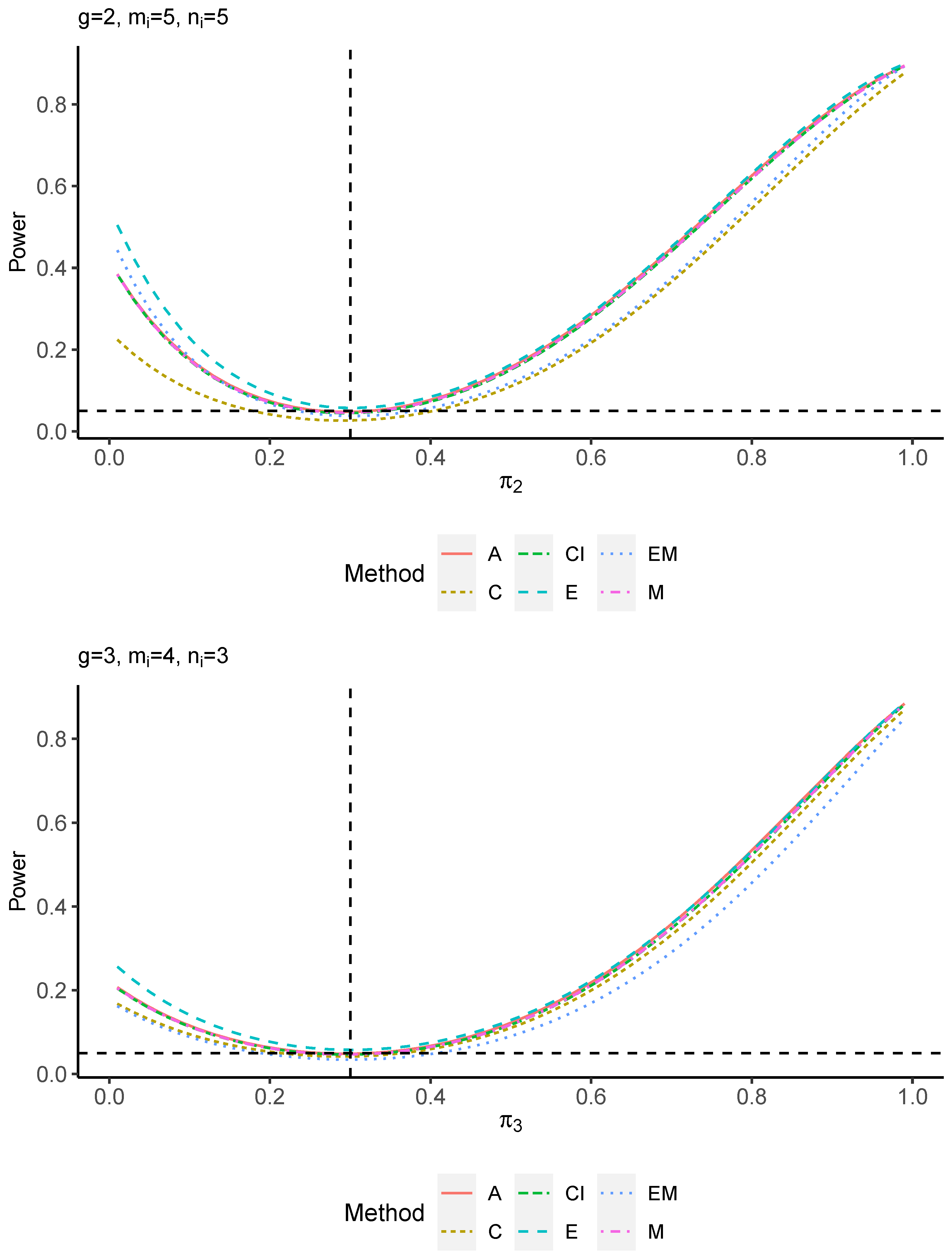
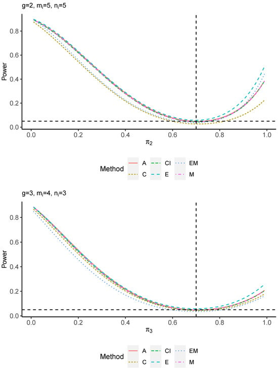
Figure A8.
Power plots for , and .
Figure A8.
Power plots for , and .
References
- Zhang, H.G.; Ying, G.S. Statistical approaches in published ophthalmic clinical science papers: A comparison to statistical practice two decades ago. Br. J. Ophthalmol. 2018, 102, 1188–1191. [Google Scholar] [CrossRef] [PubMed]
- Pearson, K.X. On the criterion that a given system of deviations from the probable in the case of a correlated system of variables is such that it can be reasonably supposed to have arisen from random sampling. London, Edinburgh, Dublin Philos. Mag. J. Sci. 1900, 50, 157–175. [Google Scholar] [CrossRef]
- Rosner, B. Statistical methods in ophthalmology: An adjustment for the intraclass correlation between eyes. Biometrics 1982, 38, 105–114. [Google Scholar] [CrossRef] [PubMed]
- Donner, A.; Banting, D. Analysis of site-specific data in dental studies. J. Dent. Res. 1988, 67, 1392–1395. [Google Scholar] [CrossRef] [PubMed]
- Donner, A. Statistical methods in ophthalmology: An adjusted chi-square approach. Biometrics 1989, 45, 605–611. [Google Scholar] [CrossRef] [PubMed]
- Ma, C.X.; Liu, S. Testing equality of proportions for correlated binary data in ophthalmologic studies. J. Biopharm. Stat. 2017, 27, 611–619. [Google Scholar] [CrossRef] [PubMed]
- Mou, K.; Li, Z. Homogeneity Test of Many-to-One Risk Differences for Correlated Binary Data under Optimal Algorithms. Complexity 2021, 2021, 6685951. [Google Scholar] [CrossRef]
- Liu, X.; Yang, Z.; Liu, S.; Ma, C.X. Exact methods of testing the homogeneity of prevalences for correlated binary data. J. Stat. Comput. Simul. 2017, 87, 3021–3039. [Google Scholar] [CrossRef]
- Liddell, D. Practical Tests of 2Times2 Contingency Tables. J. R. Stat. Soc. Ser. D (Stat.) 1976, 25, 295–304. [Google Scholar]
- Basu, D. On the Elimination of Nuisance Parameters. J. Am. Stat. Assoc. 1977, 72, 279–290. [Google Scholar] [CrossRef]
- Lloyd, C.J. Exact P-Values Discret. Model. Obtained Estim. Maximization. Aust. N. Z. J. Stat. 2008, 50, 329–345. [Google Scholar] [CrossRef]
- Ma, C.X.; Wang, H. Testing the equality of proportions for combined unilateral and bilateral data under equal intraclass correlation model. Stat. Biopharm. Res. 2022, 15, 608–617. [Google Scholar] [CrossRef]
- Fagerland, M.; Lydersen, S.; Laake, P. Statistical Analysis of Contingency Tables; CRC Press: Boca Raton, FL, USA, 2017. [Google Scholar]
- Rao, C.R. Large sample tests of statistical hypotheses concerning several parameters with applications to problems of estimation. Math. Proc. Camb. Philos. Soc. 1948, 44, 50–57. [Google Scholar]
- Berger, R.L.; Boos, D.D. P values maximized over a confidence set for the nuisance parameter. J. Am. Stat. Assoc. 1994, 89, 1012–1016. [Google Scholar] [CrossRef]
- Silvapulle, M.J. A test in the presence of nuisance parameters. J. Am. Stat. Assoc. 1996, 91, 1690–1693. [Google Scholar] [CrossRef]
- Vexler, A. Valid P-Values Expect. p-Values Revisited.Ann. Inst. Stat. Math. 2021, 73, 227–248. [Google Scholar] [CrossRef]
- Tang, N.S.; Tang, M.L.; Qiu, S.F. Testing the equality of proportions for correlated otolaryngologic data. Comput. Stat. Data Anal. 2008, 52, 3719–3729. [Google Scholar] [CrossRef]
- Mandel, E.M.; Bluestone, C.D.; Rockette, H.E.; BLATTER, M.M.; Reisinger, K.S.; Wucher, F.P.; Harper, J. Duration of effusion after antibiotic treatment for acute otitis media: Comparison of cefaclor and amoxicillin. Pediatr. Infect. Dis. J. 1982, 1, 310–316. [Google Scholar] [CrossRef] [PubMed]
- Liang, S.; Fang, K.T.; Huang, X.W.; Xin, Y.; Ma, C. Homogeneity Tests and Interval Estimations of Risk Differences for Stratified Bilateral and Unilateral Correlated Data. arXiv 2023, arXiv:2304.00162. [Google Scholar] [CrossRef]
- Lu, W.; Ning, R.; Diao, K.; Ding, Y.; Chen, R.; Zhou, L.; Lian, Y.; McAlinden, C.; Sanders, F.W.; Xia, F.; et al. Comparison of two main orthokeratology lens designs in efficacy and safety for myopia control. Front. Med. 2022, 9, 798314. [Google Scholar] [CrossRef]
- Rose, L.V.; Schulz, A.M.; Graham, S.L. Use baseline axial length measurements in myopic patients to predict the control of myopia with and without atropine 0.01%. PLoS ONE 2021, 16, e0254061. [Google Scholar] [CrossRef] [PubMed]
- Berson, E.L.; Rosner, B.; Simonoff, E. Risk factors for genetic typing and detection in retinitis pigmentosa. Am. J. Ophthalmol. 1980, 89, 763–775. [Google Scholar] [CrossRef] [PubMed]
Disclaimer/Publisher’s Note: The statements, opinions and data contained in all publications are solely those of the individual author(s) and contributor(s) and not of MDPI and/or the editor(s). MDPI and/or the editor(s) disclaim responsibility for any injury to people or property resulting from any ideas, methods, instructions or products referred to in the content. |
© 2024 by the authors. Licensee MDPI, Basel, Switzerland. This article is an open access article distributed under the terms and conditions of the Creative Commons Attribution (CC BY) license (https://creativecommons.org/licenses/by/4.0/).

