On Using Relative Information to Estimate Traits in a Darwinian Evolution Population Dynamics

Abstract

Since its inception, evolution theory has garnered much attention from the scientific community for a good reason: it theorizes how various living organisms came to be and what changes are to be expected in a certain environment. While many models of evolution have been proposed to track changes in species’ traits, not much has been said about how to calculate or estimate these traits. In this paper, using information theory, we propose an estimation method for trait parameters in a Darwinian evolution model for species with one or multiple traits. We propose estimating parameters by minimizing the relative information in a Darwinian evolution population model using either a classical gradient ascent or a stochastic gradient ascent. The proposed procedure is shown to be possible in a supervised or unsupervised learning environment, similarly to what occurs with Boltzmann machines. Simulations are provided to illustrate the method.

1. Introduction

The theory of evolution was famously championed by Darwin [1] in a publication where he stated his theory of natural selection. This theory soon became known as Darwinian evolution theory and can be construed as a series of postulates whose aim is to understand dynamical changes in organisms’ traits. In other words, understanding the mechanisms of survival or disappearance of a species entails understanding mechanisms by which species traits are passed on overtime to their offspring. From a statistical point of view, a species having multiple offspring is the realization of a random process by which a certain amount of information is passed on to an offspring. How much information or how relevant information (often found in the organism’s genome) is passed on may determine the species viability overtime. Since the paper of Vincent et al. [2] on Darwinian dynamics and evolutionary game theory, there have been many studies related to Darwinian dynamics. In Ecology in particular, Ackley et al. [3] proposed a model for competitive evolutionary dynamics, and Cushing [4] established difference equations for population dynamics. A Susceptible-Infected Darwinian model with evolutionary resistance was discussed in Cushing et al. [5]. Models for competitive species were proposed by Elaydi et al. [6]. However, the literature is very sparse on how to estimate species’ traits (information stored or passed on to offspring) from these models using readily available data.

Information theory can help design estimation methods for species traits given data. Before showing how to use information theory for such a purpose, let us mention that there are two approaches to information theory that are related, but meaning and capturing different aspects of it. Firstly, consider a given sample of data from a probability distribution that depends on a parameter. Fisher’s information [7] represents the amount of information that the sample contains about the parameter. It can be calculated as the inverse of the sampling error which is the random discrepancy between an estimate and the estimated parameter, and which arises from the sampling process itself (e.g., due to the fact that the population as a whole has not been considered). Fisher’s information is important because it is the inverse measure of the precision of a point estimate of a parameter. Indeed, the higher Fisher’s information, the more precise is the point estimate. On the other hand, when the information content (or message) of a distribution is under consideration, Shannon’s entropy [8] is used. The main difference here is that it is assumed that the content is not a parameter and therefore is not unknown. Most importantly, there is no latency relative to the population involved, unlike a sample, which is only a partial representation of a population. From Shannon’s entropy, one can define the relative entropy, which allows us to compare different distributions and thus discriminate between different types of contents of information. Even though they have different interpretations, we note that the two approaches to information are mathematically related. Indeed, Fisher’s information is the Hessian matrix with respect to the parameter of the relative entropy or Kullback–Leibler divergence. In discrete or continuous Darwinian dynamics, the main assumption is that of a deterministic relationship between inputs and outputs. As we stated above, the transmission of traits from parents to offspring is, in fact, a random process and should be analyzed as such. This assumes that there is a stochastic relationship between inputs and outputs via a network of connections often referred to as weights.

More precisely, say u is the vector of inputs and v the vector of outputs with network connections matrix W. If input and output samples $({\mathbf{u}}_s,{\mathbf{v}}_s),1\le s\le S$ are both available, the stochastic relationship between inputs and outputs is described as $\mathbb{P}\left(\mathbf{v}\right|\mathbf{u},\mathbf{W})$, which is the probability that input u generates output v when the weight matrix of the network is W. In supervised learning, the goal is to match as closely as possible the input–output distribution $\mathbb{P}\left(\mathbf{v}\right|\mathbf{u},\mathbf{W})$ with the probability distribution $\mathbb{P}\left(\mathbf{v}\right|\mathbf{u})$ related to the samples $({\mathbf{u}}_s,{\mathbf{v}}_s)$, by adjusting the weights W in a feedforward manner. In unsupervised learning, it is assumed that output samples are not given and only input samples $\left({\mathbf{u}}_s\right),1\le s\le S$ are given. However, using an appropriate energy function, one can obtain the joint probability distribution $\mathbb{P}(\mathbf{u},\mathbf{v},\mathbf{W})$ and infer from rules of probability that $\mathbb{P}(\mathbf{u},\mathbf{W})={\sum }_{\mathbf{v}}\mathbb{P}(\mathbf{u},\mathbf{v},\mathbf{W})$. The goal in unsupervised learning is therefore to match $\mathbb{P}(\mathbf{u},\mathbf{W})$ as closely as possible to the probability distribution $\mathbb{P}\left(\mathbf{u}\right)$ related to samples $\left({\mathbf{u}}_s\right),1\le s\le S$, by adjusting the weights W in a feedforward manner. Feedforward techniques require the minimization of an appropriate objective function, and since we are dealing with probability distributions, the Kullback–Leibler divergence seems to be the best choice of objective function.

In this paper, our focus is on using relative information or entropy to estimate trait parameters in a Darwinian population dynamics model. The procedure we propose is similar to what occurs in a Boltzmann machine. The remainder of the paper is organized as follows: In Section 2, we make a brief overview of Fisher’s information theory, entropy and relative as it pertains to mathematical statistics. In Section 3, we discuss how to computationally estimate trait parameters of discrete Darwinian models in supervised and unsupervised environments by maximizing the relative information or Kullback–Leibler divergence. Finally, in Section 4, we make some concluding remarks.

2. Review of Information Theory

In this light review of information theory, we mention Fisher’s information only for self-containment sake. As for Fisher’s information and evolution dynamics, the reader can refer to [9] for a deeper analysis. For ease of analysis and comprehension, the assumptions and notations below are along the lines of that work.

2.1. Fisher’s Information Theory

Let $G(x,\mathsf{\Theta })$ be the probability density of a random variable X, continuous or discrete on an open set $\mathcal{X}\times \mathsf{\Omega }\subset \mathbb{R}\times {\mathbb{R}}^n$. Here $\mathsf{\Theta }=({\theta }_1,{\theta }_2,\cdots ,{\theta }_n)$ is either a single parameter or a vector of parameters.

In the sequel, we consider the following assumptions on the function $G(x,\mathsf{\Theta })$:

A₁ :

The support $\left\{x\in \mathcal{X}:G(x,\mathsf{\Theta })\ne 0\right\}$ of G is independent of $\mathsf{\Theta }$.

A₂ :

$G(·,\mathsf{\Theta })$ is nonnegative and $G\in L^1\left(\mathcal{X}\right)$ for all $\mathsf{\Theta }\in \mathsf{\Omega }$.

A₃ :

$G(x,·)\in C^2\left(\mathsf{\Omega }\right)$, the set of continuously and twice differentiable functions of $\mathsf{\Theta }$, for all $x\in \mathcal{X}$.

The first assumption is to discard from consideration the uniform distribution $G(x,\theta )=\frac{1}{\theta }$ whose support is $(0,\theta )$. The second and third assumptions allow the well-definiteness of $\lambda (x,\theta )=\ln \left(G\right(x,\theta \left)\right)$, its first derivative or score function $g(x,\mathsf{\Theta })={\nabla }_{\theta }\lambda (x,\mathsf{\Theta })$ and its second derivative $h(x,\mathsf{\Theta })={\nabla }_{\mathsf{\Theta }}g(x,\mathsf{\Theta })={\nabla }_{\mathsf{\Theta }}^2\lambda (x,\mathsf{\Theta })$. In the sequel, the expected value of a random variable X is denoted as $\mathbb{E}\left[X\right]$.

Definition 1.

Given a random variable X with density function $G(x,\mathsf{\Theta })$ satisfying $A_1$ and $A_2$, Fisher’s information of X is defined as

$$I\left(\mathsf{\Theta }\right)={\mathbb{E}}_X\left[{\left(g(X,\theta )\right)}^2\right]=-{\mathbb{E}}_X\left[h(X,\mathsf{\Theta })\right].$$

(1)

When $\mathsf{\Theta }$ is vector of more than one coordinates, Fisher’s information is a symmetric positive definite (thus invertible) matrix $I\left(\mathsf{\Theta }\right)={\left(I_{kl}\left(\mathsf{\Theta }\right)\right)}_{1\le k,l\le n}$, where

$$I_{kl}={\mathbb{E}}_X\left[\frac{{\partial }^2\lambda (X,\mathsf{\Theta })}{\partial {\theta }_k\partial {\theta }_l}\right],\mathrm{for} 1\le k,l\le n.$$

(2)

Fisher’s information $I\left(\mathsf{\Theta }\right)$ represents the amount of information contained in an estimator of $\mathsf{\Theta }$, given data X.

2.2. Entropy and Relative Entropy

Let us start by recalling the following definition of Shannon’s entropy and that of the Kullback–Leibler divergence or relative entropy.

Definition 2.

Let μ be a probability distribution defined on a sample space Ω. Then entropy of μ is given as

$$H\left(\mu \right)=-{\mathbb{E}}_{\mu }\left[\ln \left[\mu \right]\right]=\left\{\begin{array}{cc}{\displaystyle -\sum _{\theta \in \mathsf{\Omega }}\mu \left(\theta \right)\ln \left(\mu \left(\theta \right)\right),}\hfill & \mathit{if}\mu \mathit{is}\mathit{discrete}\hfill \\ {\displaystyle -{\int }_{\theta \in \mathsf{\Omega }}\mu \left(\theta \right)\ln \left(\mu \left(\theta \right)\right)d\theta ,}\hfill & \mathit{if}\mu \mathit{is}\mathit{continuous}\hfill \end{array}\right..$$

(3)

Definition 3.

Suppose μ and ν are two probability distributions defined on a sample space Ω. Then, the Kullback–Leibler divergence or relative information $D(\mu ,\nu )$ of μ relative to a fixed ν is given as

$$D_{KL}(\mu ,\nu )={\mathbb{E}}_{\mu }\left[\frac{\ln \left(\mu \right)}{\ln \left(\nu \right)}\right]=\left\{\begin{array}{cc}{\displaystyle \sum _{\theta \in \mathsf{\Omega }}\mu \left(\theta \right)\ln \left(\frac{\mu \left(\theta \right)}{\nu \left(\theta \right)}\right),}\hfill & \mathit{if}\mu \mathit{and}\nu \mathit{are}\mathit{discrete}\hfill \\ {\displaystyle {\int }_{\theta \in \mathsf{\Omega }}\mu \left(\theta \right)\ln \left(\frac{\mu \left(\theta \right)}{\nu \left(\theta \right)}\right)d\theta ,}\hfill & \mathit{if}\mu \mathit{and}\nu \mathit{are}\mathit{continuous}\hfill \end{array}\right..$$

(4)

There is an obvious connection between entropy and relative entropy:

$$D_{KL}(\mu ,\nu )=-{\mathbb{E}}_{\mu }\left[\ln \left(\nu \right)\right]-H\left(\mu \right).$$

We notice that when $\mu =\nu$, we have that $D_{KL}(\mu ,\nu )=0$. It is known that Fisher’s information induces a Riemannian metric ([10,11]) defined on a statistical manifold, that is, a smooth manifold whose points are probability measures defined on a probability space. It therefore represents the “informational” discrepancy between measurements. As such, it is related to the Kullback–Leibler divergence (KL), used typically to assess the difference between two probability distributions. Indeed, to see this, let $\theta ,{\theta }_0\in \mathsf{\Omega }$. Let us use a second-order Taylor expansion in $\mu$. Then we will obtain

$$\begin{array}{ccc}\hfill D_{KL}(\mu ,\nu )& =& D_{KL}(\mu ,\nu ){|}_{\mu \left(\theta \right)=\nu \left(\theta \right)}\hfill \\ & +& {\nabla }_{\theta }\left(D_{KL}(\mu ,\nu )\right){|}_{\mu \left(\theta \right)=\nu \left(\theta \right)}+\frac{1}{2}{(\theta -{\theta }_0)}^T\mathcal{H}\left(\theta \right)(\theta -{\theta }_0)+\mathrm{O}\left({(\theta -{\theta }_0)}^3\right).\hfill \end{array}$$

From the above observation, we have $D(\mu ,\nu ){|}_{\mu =\nu }=0$. We also have

$$\begin{array}{ccc}\hfill {\nabla }_{\theta }\left(D_{KL}(\mu ,\nu )\right)& =& \frac{\partial }{\partial \theta }{\mathbb{E}}_{\mu }\left[\frac{\ln \left(\mu \right)}{\ln \left(\nu \right)}\right]\hfill \\ & =& {\mathbb{E}}_{\mu }\left[\frac{\partial }{\partial \theta }\left(\frac{\ln \left(\mu \right)}{\ln \left(\nu \right)}\right)\right]\hfill \\ & =& {\mathbb{E}}_{\partial \mu }\left[\frac{\ln \left(\mu \right)}{\ln \left(\nu \right)}\right]+{\mathbb{E}}_{\nu }\left[\frac{\partial }{\partial \theta }\left(\frac{\mu }{\nu }\right)\right].\hfill \end{array}$$

It follows that ${\displaystyle {\nabla }_{\theta }\left(D_{KL}(\mu ,\nu )\right){|}_{\mu \left(\theta \right)=\nu \left(\theta \right)}=0}$. We conclude by noticing that the Hessian matrix $\mathcal{H}\left(\theta \right)={\nabla }_{\theta }^2{D}_{KL}(\mu ,\nu ){|}_{\mu \left(\theta \right)=\nu \left(\theta \right)}={\mathbb{E}}_{\mu }\left[\frac{{\partial }^2}{\partial {\theta }_k\partial {\theta }_l}\ln \left(\mu \left(\theta \right)\right)\right]=I\left(\theta \right)$. Therefore, if $\mu =\mu \left(\theta \right)$ and $\nu =\mu \left({\theta }_0\right)$ are infinitesimally close to each other, that is,

$$\mu \left(\theta \right)=\mu \left({\theta }_0\right)+\sum _k\Delta {\theta }_k\frac{\partial }{\partial {\theta }_k}\mu \left(\theta \right){|}_{\theta ={\theta }_0},$$

(5)

we have

$$D_{KL}(\mu ,\nu )=\frac{1}{2}\sum _{kl}\Delta {\theta }_k\Delta {\theta }_l{I}_{kl}\left(\theta \right)+\mathrm{O}(\Delta {\theta }^3).$$

(6)

There is an interesting discussion in the finite case in [12]. Indeed, suppose that $\mathsf{\Omega }$ is a finite set with cardinality n. Let $\mathsf{\Theta }=({\theta }_1,{\theta }_2,\cdots ,{\theta }_n)$ and let $\mathsf{\Lambda }\left(\mathsf{\Omega }\right)$ be the set of all probability measures on $\mathsf{\Omega }$, and $S_n\left(\mathsf{\Omega }\right)$ be the simplex $S_n\left(\mathsf{\Omega }\right)=\left\{\mathsf{\Theta }\in \mathsf{\Omega }:{\sum }_{i=1}^n{\theta }_i=1\right\}$. There is a isometry $\phi :\mathsf{\Lambda }\left(\mathsf{\Omega }\right)\to S_n\left(\mathsf{\Omega }\right)$ defined as $\phi \left(\mu \right)=(\mu \left(1\right),\mu \left(2\right),\cdots ,\mu \left(n\right))=({\theta }_1,{\theta }_2,\cdots ,{\theta }_n)$. In this case, Fisher’s information components become

$$\begin{array}{ccc}\hfill I_{kl}\left(\theta \right)& =& {\mathbb{E}}_{\mu }\left[\frac{{\partial }^2}{\partial {\theta }_k\partial {\theta }_l}\ln \left(\mu \left(\theta \right)\right)\right]=\sum _{j=1}^n{\theta }_j\frac{1}{{\theta }_k}{\delta }_{kj}\frac{1}{{\theta }_l}{\delta }_{lj}=\frac{1}{{\theta }_k}{\delta }_{kl},\hfill \end{array}$$

where ${\delta }_{kl}$ is the Kronecker symbol. It follows that

$$\frac{{\partial }^{2}D(\mu ,{\mu }_0)}{\partial {\theta }_k\partial {\theta }_l}=\frac{1}{{\theta }_k}{\delta }_{kl}.$$

The interpretation of the latter is Fisher’s fundamental theorem (see [7]) and Kimura’s maximal principle (see [13]) in terms of Fisher information: natural selection forms a gradient with respect to an information measure, and hence locally has the direction of maximal information increase. The rate of change of the mean fitness of the population is given by the information variance.

Let us highlight some of these facts by calculating the KL divergence $D_{KL}({\mathsf{\Theta }}_1,{\mathsf{\Theta }}_t)$ between distributions $\nu =\mathbb{P}\left({\mathsf{\Theta }}_1\right)$ and $\mu =\mathbb{P}\left({\mathsf{\Theta }}_t\right)$ of ${\mathsf{\Theta }}_1$ and ${\mathsf{\Theta }}_t$, respectively, and $D_{KL}({\mathsf{\Theta }}_t,{\mathsf{\Theta }}_{t+1})$ between the probability distributions $\nu =\mathbb{P}\left({\mathsf{\Theta }}_t\right)$ and $\mu =\mathbb{P}\left({\mathsf{\Theta }}_{t+1}\right)$ of ${\mathsf{\Theta }}_t$ and ${\mathsf{\Theta }}_{t+1}$, respectively, for $t=1,2,\cdots ,n$. See Figure 1 below. We will use the same parameters as above with the same starting points for $\theta$ in the algorithm.

Figure 1. In (a) $D({\mathsf{\Theta }}_t,{\mathsf{\Theta }}_{t+1})$; (b) $D({\mathsf{\Theta }}_1,{\mathsf{\Theta }}_{t+1})$ for $t=1,2,\cdots ,15$. In the (a), convergence to zero means that the distributions of ${\mathsf{\Theta }}_t$ and ${\mathsf{\Theta }}_{t+1}$ are similar. In (b), convergence to about 8.7 means that the distributions of ${\mathsf{\Theta }}_t$ are no more different from each other, making their KL divergence from the distribution of ${\mathsf{\Theta }}_1$ constant. In both cases, this is an indication that Fisher’s information has been maximized or that the variances of the estimates are the same and very small.

The minimization of $D_{KL}({\mathsf{\Theta }}_t,{\mathsf{\Theta }}_{t+1})$ and the maximization of $D_{KL}({\mathsf{\Theta }}_1,{\mathsf{\Theta }}_t)$ both occur when Fisher’s information is maximal or when the variance of the estimator is minimal. From a dynamical system perspective, this occurs when the fixed point $(e^{-1},e)$ has been attained. This means that the KL divergence can be used to determine the critical points of a discrete Darwinian model. Therefore, there is a dichotomy between the problems of minimizing $D({\mathsf{\Theta }}_t,{\mathsf{\Theta }}_{t+1})$ and maximizing $D_{KL}({\mathsf{\Theta }}_1,{\mathsf{\Theta }}_t)$. This amounts to matching the probability distributions $\mathbb{P}\left({\mathsf{\Theta }}_t\right)$ and $\mathbb{P}\left({\mathsf{\Theta }}_{t+1}\right)$ as closely as possible. When this happens, we know from above that we will have $D_{KL}({\mathsf{\Theta }}_t,{\mathsf{\Theta }}_{t+1})\approx 0$, which in turn will mean that the fixed points of the discrete Darwinian model have been attained. To that end, we will discuss how to accomplish this with machine learning approaches, namely under supervised and unsupervised learning.

3. Evolution Population Dynamics and Relative Information

3.1. Single Darwinian Population Model with Multiple Traits

Now suppose we are in the presence of one species with density x possessing n traits given by the vector $\mathsf{\Theta }=({\theta }_1,{\theta }_2,\cdots ,{\theta }_n)$ and a vector $U=(u_1,u_2,\cdots ,u_n)$. We will consider the following:

(H₁)

$b\left(\mathsf{\Theta }\right)=b_0\exp \left({\displaystyle -\sum _{i=1}^n\frac{{\theta }_i^2}{2w_i^2}}\right)$ is the joint distribution of the independent traits ${\theta }_i$, each with mean 0 and variance $w_i^2$.

(H₂)

$c_U\left(\mathsf{\Theta }\right)=c_0\exp \left({\displaystyle -\sum _{i=1}^n{\kappa }_i({\theta }_i-u_i)}\right)$.

(H₃)

The density of $x_t$ is given as $G(x,\mathsf{\Theta },U)=b\left(\mathsf{\Theta }\right)\exp (-c_U\left(\mathsf{\Theta }\right)x)$ at $t=1$.

Under $H_1-H_3$, we will consider the discrete dynamical system

$$\left\{\begin{array}{cc}{x}_{t+1}\hfill & =x_{t}G(x_t,{\mathsf{\Theta }}_t,U_t)\hfill \\ {\mathsf{\Theta }}_{t+1}\hfill & ={\mathsf{\Theta }}_t+\mathsf{\Sigma }g(x_t,{\mathsf{\Theta }}_t,U_t)\hfill \end{array}\right.,$$

(7)

where

$$\mathsf{\Sigma }=\left(\begin{array}{cccc}{\sigma }_{11}& {\sigma }_{12}& \cdots & {\sigma }_{1n}\\ {\sigma }_{21}& {\sigma }_{22}& \cdots & {\sigma }_{2n}\\ ⋮& ⋮& \cdots & ⋮\\ {\sigma }_{n1}& {\sigma }_{n2}& \cdots & {\sigma }_{nn}\end{array}\right).$$

(8)

Remark 1.

We note that in the context of Darwinian population dynamics, $G(x_t,{\mathsf{\Theta }}_t,U_t)$ is the population growth rate, $b\left(\mathsf{\Theta }\right)$ represents the birth rate, while $c_U\left(\mathsf{\Theta }\right)$ is the intra-specific competition function. Σ represents the covariance matrix of the distribution of traits among phenotypes of the species.

In this section, we propose two approaches to estimate the traits vector $\mathsf{\Theta }$ in a Darwinian model, using relative information.

3.2. Supervised and Unsupervised Learning

Supervised and unsupervised learning are two types of machine learning techniques whose ultimate aim is to learn the best possible connections between a set of inputs and outputs. In supervised learning, the inputs and outputs are presented to a system that learns the best possible connections between inputs and outputs. In an unsupervised learning environment, only inputs are presented and the system learns and describes the best possible outputs that would be related to the inputs. Let us note that the distribution of ${\mathsf{\Theta }}_t$ depends on $X_t,K=({\kappa }_1,{\kappa }_2,\cdots ,{\kappa }_n),W=(w_1,w_2,\cdots ,w_n)$, and $U=(u_1,u_2,\cdots ,u_n)$.

In the sequel, we propose a machine learning approach for the estimation of trait vector $\mathsf{\Theta }$. We show in particular that depending on the amount of information available, machine learning approaches are possible. To that end, learning schemes for supervised and unsupervised learning are designed to estimate both W and K, which are the key parameters in the Darwinian model (7) proposed above. In fact, once the vectors W and K have been estimated, data available on $X_t$ and the second equation in (7) are used to evaluate ${\mathsf{\Theta }}_t^{\mathrm{estimated}}$, the estimated value of $\mathsf{\Theta }$. In supervised learning, the values of ${\mathsf{\Theta }}_t^{\mathrm{estimated}}$ should match closely with their sample counterparts ${\mathsf{\Theta }}_t^{\mathrm{samples}}$. In unsupervised learning, in the absence of sample data ${\mathsf{\Theta }}_t^{\mathrm{samples}}$, the estimated values ${\mathsf{\Theta }}_t^{\mathrm{estimated}}$ should serve as actual values for ${\mathsf{\Theta }}_t$, the vector of traits.

3.2.1. Supervised Learning

Let $n,T$ and M be given positive integers. In supervised learning, we are given a sample of inputs/outputs sample in the form

$$\left\{\left(X_t^{\left(m\right)},{\mathsf{\Theta }}_t^{\left(m\right)}\right),t=1,2\cdots ,T;m=1,2\cdots ,M\right\},$$

where each ${\mathsf{\Theta }}_t^{\left(m\right)}$ is a $1\times N$ vector. This means that in this case, we already know the inputs that generate the solution of the system (7). The probability $\mathbb{P}\left(X_t\right|{\mathsf{\Theta }}_t,W,K)$ of $X_t$ given ${\mathsf{\Theta }}_t,W,K$ is

$$\mathbb{P}\left(X_t\right|{\mathsf{\Theta }}_t,W,K)=b_0{e}^{-b(X_t,{\mathsf{\Theta }}_t,W,K)}.$$

(9)

Therefore, using known techniques of conditional probabilities, we have

$$\mathbb{P}\left({\mathsf{\Theta }}_t\right|X_t,W,K)=\frac{\mathbb{P}\left(X_t\right|{\mathsf{\Theta }}_t,W,K)\mathbb{P}\left({\mathsf{\Theta }}_t\right)}{Z},$$

(10)

where

$$Z=\sum _{{\mathsf{\Theta }}_t}\mathbb{P}\left(X_t\right|{\mathsf{\Theta }}_t,W,K)\mathbb{P}\left({\mathsf{\Theta }}_t\right).$$

Since we are trying to estimate traits, in supervised learning, the goal will be to determine how well $\mathbb{P}\left({\mathsf{\Theta }}_{t+1}\right|X_{t+1},W,K)$ matches $\mathbb{P}\left({\mathsf{\Theta }}_t\right|X_t)$. Since these are distributions, we use the Kulback–Leibler (KL) divergence

$$\begin{array}{cc}\hfill D_{KL}(\mathbb{P}\left({\mathsf{\Theta }}_t\right|X_t),\mathbb{P}\left({\mathsf{\Theta }}_{t+1}\right|X_{t+1},W,K))=& -\sum _{{\theta }_t}\mathbb{P}\left({\mathsf{\Theta }}_t|X_t\right)\ln \left(\mathbb{P}\left({\mathsf{\Theta }}_{t+1}\right|X_{t+1},W,K)\right)-H\left({\mathsf{\Theta }}_t\right|X_t),\hfill \end{array}$$

(11)

where

$${\displaystyle H\left({\mathsf{\Theta }}_t\right|X_t)=-\sum _{{\theta }_t}\mathbb{P}\left({\mathsf{\Theta }}_t\right|X_t)\ln \left(\mathbb{P}\left({\mathsf{\Theta }}_t\right|X_t)\right)}$$

is the entropy of the distribution of ${\mathsf{\Theta }}_t|X_t$. At the sample level for given M samples, the average of KL divergence is given as

$$⟨D_{KL}(\mathbb{P}\left({\mathsf{\Theta }}_t\right|X_t),\mathbb{P}\left({\mathsf{\Theta }}_{t+1}\right|X_{t+1},W,K))⟩=-\frac{1}{M}\left[\sum _{m=1}^M\ln \left(\mathbb{P}\left({\mathsf{\Theta }}_{t+1}^{\left(m\right)}\right|X_{t+1}^{\left(m\right)},W,K)\right)+H\left[{\mathsf{\Theta }}_t^{\left(m\right)}|X_t^{\left(m\right)}\right]\right].$$

(12)

We minimize the quantity on the right-hand side of (12), using a stochastic gradient descent scheme, by updating the weight vectors W and K, respectively. Hence, the following result on supervised learning.

Theorem 1.

Suppose that $X_t,W$, and K are as above and that we have input/output sample $\left\{\left(X_t^{\left(m\right)},{\mathsf{\Theta }}_t^{\left(m\right)}\right),t=1,2,\cdots ,T,m=1,2,\cdots ,M\right\}$. The minimization process of the KL divergence can be achieved with a classic gradient ascent algorithm for weights W and K with an update scheme given as

$$\left\{\begin{array}{cc}{w}_{l,new}\hfill & {\displaystyle =w_{l,old}+{\alpha }_W\frac{\partial \ln \left(\mathbb{P}\left({\mathsf{\Theta }}_{t+1}^{\left(m\right)}\right|X_{t+1}^{\left(m\right)},W,K)\right)}{\partial w_l}}\hfill \\ {\kappa }_{l,new}\hfill & {\displaystyle ={\kappa }_{l,old}+{\alpha }_K\frac{\partial \ln \left(\mathbb{P}\left({\mathsf{\Theta }}_{t+1}^{\left(m\right)}\right|X_{t+1}^{\left(m\right)},W,K)\right)}{\partial {\kappa }_l}}\hfill \end{array}\right.,$$

(13)

where ${\alpha }_w,{\alpha }_{\kappa }>0$ are the learning rates of W and K, respectively, and ${\displaystyle \frac{\partial \ln \left(\mathbb{P}\left({\mathsf{\Theta }}_{t+1}^{\left(m\right)}\right|X_{t+1}^{\left(m\right)},W,K)\right)}{\partial x}}$ for  $x=w_l,{\kappa }_l$ is given in the Appendix A.

Corollary 1.

Under the assumptions of Theorem 1 above, the minimization process of the KL divergence can be achieved more efficiently with a stochastic gradient ascent algorithm for weights W and K with an update scheme given as

$$\left\{\begin{array}{cc}{w}_{l,new}\hfill & {\displaystyle =w_{l,old}-{\alpha }_W\left[\frac{\partial b(X_{t+1}^{\left(m\right)},{\mathsf{\Theta }}_{t+1}^{\left(m\right)},W,K)}{\partial w_l}-\frac{\partial b(X_{t+1}^{\left(m\right)},{\mathsf{\Theta }}_t^{\left(m\right)},W,K)}{\partial w_l}\right]}\hfill \\ {\kappa }_{l,new}\hfill & {\displaystyle ={\kappa }_{l,old}-{\alpha }_K\left[\frac{\partial b(X_{t+1}^{\left(m\right)},{\mathsf{\Theta }}_{t+1}^{\left(m\right)},W,K)}{\partial {\kappa }_l}-\frac{\partial b(X_{t+1}^{\left(m\right)},{\mathsf{\Theta }}_t^{\left(m\right)},W,K)}{\partial {\kappa }_l}\right]}\hfill \end{array}\right..$$

(14)

where ${\alpha }_w,{\alpha }_{\kappa }>0$ are the learning rates of W and K, respectively.

Remark 2.

One could use Jeffrey’s prior as the probability distribution $\mathbb{P}\left({\mathsf{\Theta }}_t\right)$ of ${\mathsf{\Theta }}_t$ if no other information about its distribution is given. In this case, $\mathbb{P}\left({\mathsf{\Theta }}_t\right)\propto \frac{1}{\sqrt{det\left(I\left({\mathsf{\Theta }}_t\right)\right)}}$, where $det\left(A\right)$ is the determinant of the matrix A. We discussed in [9] that Fisher’s information matrix for such a system depends on both W and K. This means that a Jeffrey’s prior is advisable only for algorithm initialization; otherwise, from Equation (10), the updating scheme would have to be changed according to the dependence of $\mathbb{P}\left({\mathsf{\Theta }}_t\right)$ on both W and K. In fact, in this case, one would need to consider the respective partial derivatives $\frac{\partial \ln \left(\mathbb{P}\left({\theta }_t\right)\right)}{\partial x}=-\frac{1}{2}\frac{\frac{\partial }{\partial x}det\left(I\left({\theta }_t\right)\right)}{det\left(I\left({\theta }_t\right)\right)}$, for $x=w_l,{\kappa }_l$, which significantly increases the complexity of the problem.

3.2.2. Unsupervised Learning

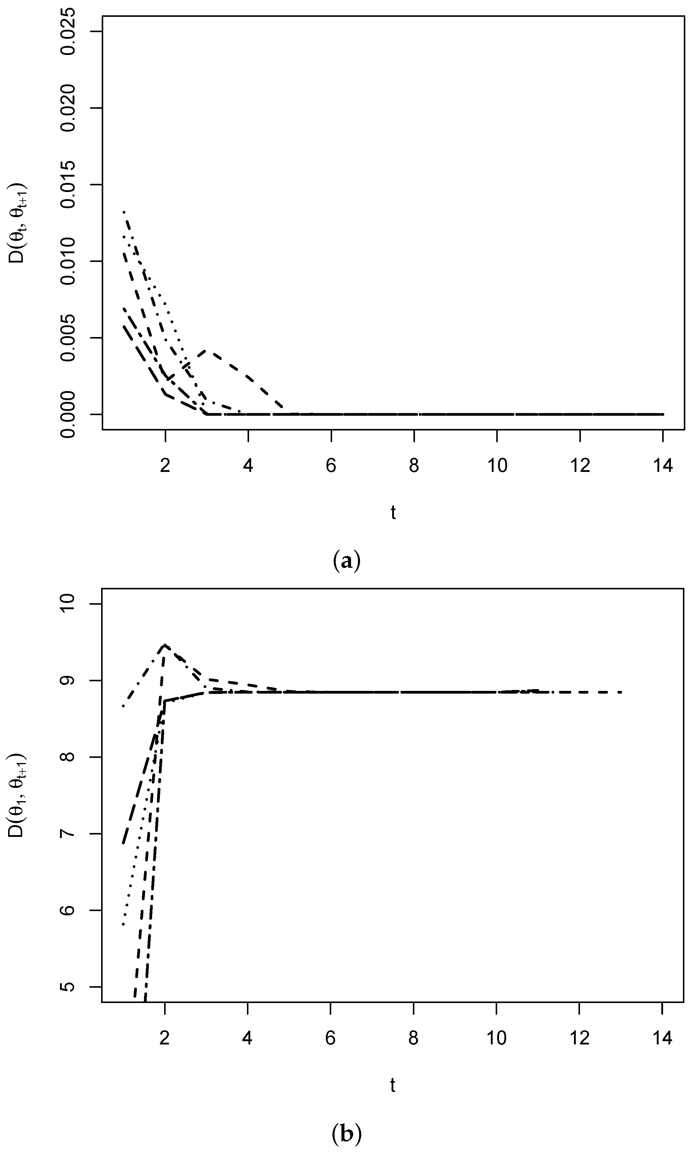
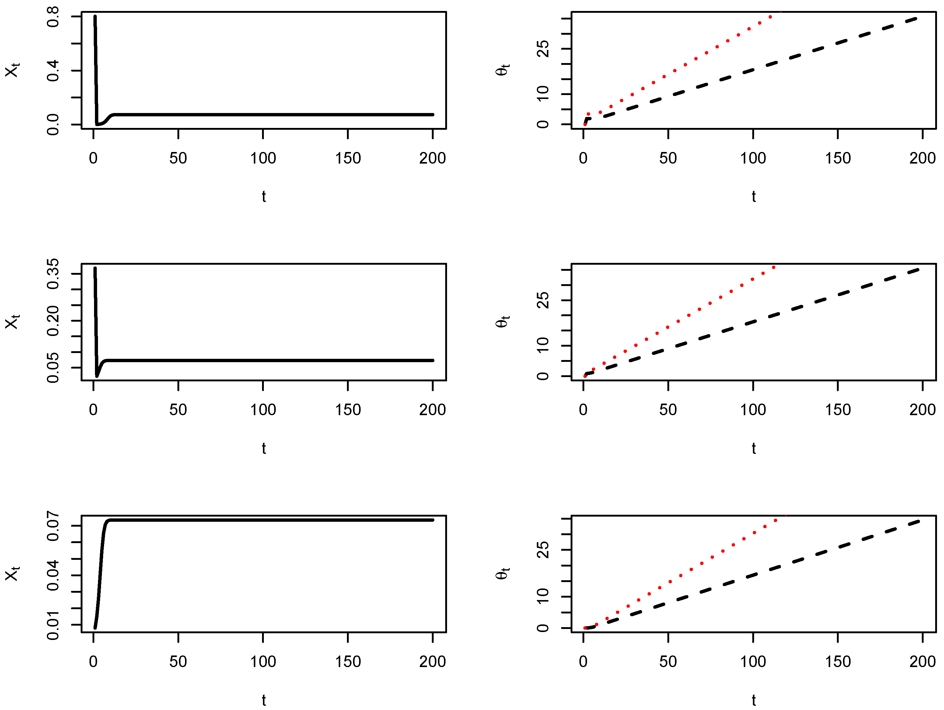
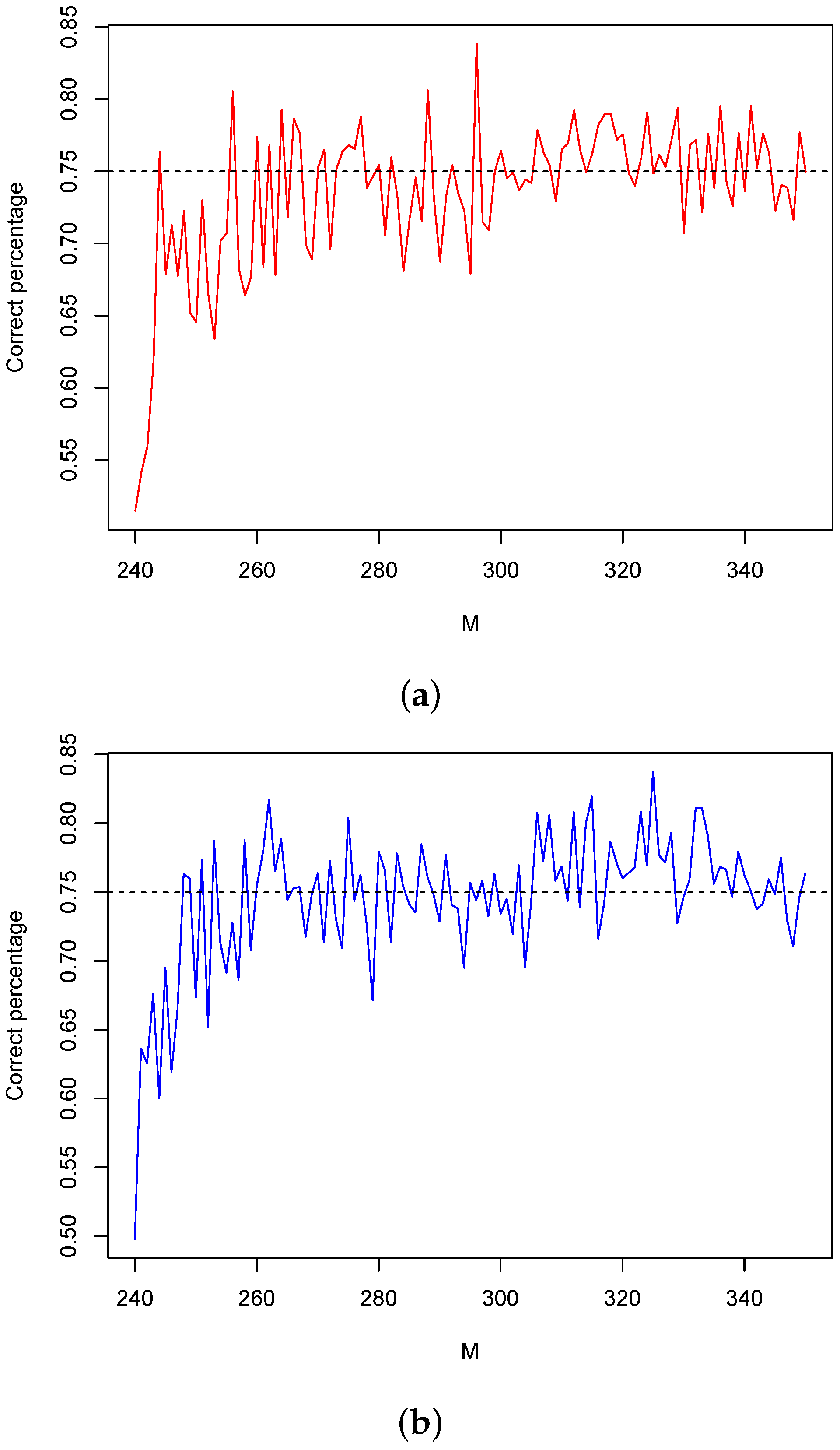
Now, we assume that $X_t,W$, and K are as above and only a sample of inputs $\left\{X_t^{\left(m\right)},m\in \left\{1,2,\cdots ,M\right\}\right\}$ is given. Since ${\mathsf{\Theta }}_t^{\left(m\right)}$ is not given, we cannot use the learning scheme above. We have to design a method that only depends on $X_t^{\left(m\right)},W$ and K. We assume that the joint probability $\mathbb{P}(X_t,{\mathsf{\Theta }}_t,W,K)$ of $X_t$ and ${\mathsf{\Theta }}_t$ is

$$\mathbb{P}(X_t,{\mathsf{\Theta }}_t,W,K)=\frac{1}{Z}{e}^{-b(X_t,{\mathsf{\Theta }}_t,W,K)},$$

(15)

where Z is the constant ${\displaystyle Z=\sum _{X_t,{\mathsf{\Theta }}_t}{e}^{-b(X_t,{\mathsf{\Theta }}_t,W,K)}}$.

In unsupervised learning, we would like to determine how well $\mathbb{P}(X_{t+1},W,K)$ matches $\mathbb{P}\left(X_t\right)$. Since these are distributions, we use the Kulback–Leibler (KL) divergence

$$\begin{array}{cc}\hfill D_{KL}(\mathbb{P}\left(X_t\right),\mathbb{P}(X_{t+1},W,K))=& -\sum _{X_t}\mathbb{P}\left(\left(X_t\right)\right)\ln \left(\mathbb{P}(X_{t+1},W,K)\right)-H\left(X_t\right),\hfill \end{array}$$

(16)

where ${\displaystyle H\left(X_t\right)=-\sum _{X_t}\mathbb{P}\left(X_t\right)\ln \left(\mathbb{P}\left(X_t\right)\right)}$ is the entropy of the distribution of $X_t$. At the sample level, and for given M samples from the random variable $X_t$, the average of KL divergence is given as

$$⟨D_{KL}(\mathbb{P}\left(X_t\right),\mathbb{P}(X_{t+1},W,K))⟩=-\frac{1}{M}\left[\sum _{m=1}^M\ln \left(\mathbb{P}(X_{t+1}^{\left(m\right)},W,K)\right)+H\left(X_t^{\left(m\right)}\right)\right].$$

(17)

Similarly, as above, we minimize the quantity on the right-hand side of (17), using a stochastic gradient descent scheme, by updating the weight vectors W and K, respectively. Hence, the following result is on unsupervised learning.

Theorem 2.

Suppose that $X_t,W$, and K are as above and that we have input/output sample $\left\{X_t^{\left(m\right)},t=1,2,\cdots ,T,m=1,2,\cdots ,M\right\}$. The minimization process of the KL divergence can be achieved with a classic gradient ascent algorithm for weights W and K with an update scheme given as

$$\left\{\begin{array}{cc}{w}_{l,new}\hfill & {\displaystyle =w_{l,old}+{\alpha }_W\frac{\partial \ln \left(\mathbb{P}(X_{t+1}^{\left(m\right)},W,K)\right)}{\partial w_l}}\hfill \\ {\kappa }_{l,new}\hfill & {\displaystyle ={\kappa }_{l,old}+{\alpha }_K\frac{\partial \ln \left(\mathbb{P}(X_{t+1}^{\left(m\right)},W,K)\right)}{\partial {\kappa }_l}}\hfill \end{array}\right..$$

(18)

where ${\alpha }_w,{\alpha }_{\kappa }>0$ are the learning rates of W and K, respectively, and ${\displaystyle \frac{\partial \ln \left(\mathbb{P}(X_{t+1}^{\left(m\right)},W,K)\right)}{\partial x}}$, for $x=w_l,{\kappa }_l$ is given in the Appendix A.

Corollary 2.

Under the hypotheses of Theorem 2 above, the minimization process of the KL divergence can be achieved more efficiently with a stochastic gradient ascent algorithm for weights W and K with an update scheme given as

$$\left\{\begin{array}{cc}{w}_{l,new}\hfill & {\displaystyle =w_{l,old}-{\alpha }_W\left[\frac{\partial b(X_{t+1}^{\left(m\right)},{\mathsf{\Theta }}_t^{\left(m\right)},W,K)}{\partial w_l}-\frac{\partial b(X_t^{\left(m\right)},{\mathsf{\Theta }}_t^{\left(m\right)},W,K)}{\partial w_l}\right]}\hfill \\ {\kappa }_{l,new}\hfill & {\displaystyle ={\kappa }_{l,old}-{\alpha }_K\left[\frac{\partial b(X_{t+1}^{\left(m\right)},{\mathsf{\Theta }}_t^{\left(m\right)},W,K)}{\partial {\kappa }_l}-\frac{\partial b(X_t^{\left(m\right)},{\mathsf{\Theta }}_t^{\left(m\right)},W,K)}{\partial {\kappa }_l}\right]}\hfill \end{array}\right.,$$

(19)

where ${\alpha }_w,{\alpha }_{\kappa }>0$ are the learning rates of W and K, respectively.

Remark 3.

1. 

We observe that since $D_{KL}(\mathbb{P}\left({\mathsf{\Theta }}_t\right|X_t),\mathbb{P}\left({\mathsf{\Theta }}_{t+1}\right|X_{t+1},W,K))$ is an expectation with respect to ${\mathsf{\Theta }}_t|X_t$ (see Definition 3 above), then the right-hand-side of Equation (12)  is a Riemann sum for  $D_{KL}(\mathbb{P}\left({\mathsf{\Theta }}_t\right|X_t),\mathbb{P}\left({\mathsf{\Theta }}_{t+1}\right|X_{t+1},W,K))$.

2. 

Similarly, $D_{KL}(\mathbb{P}(X_t,\mathbb{P}(X_{t+1},W,K))$ is an expectation with respect to the random variable $X_t$, therefore the right-hand-side of Equation (17) is one of its Riemann sum.

Remark 4.

We note that there is a subtle difference between Equations (14) and (19), but an important one. In Equation (14), all the data are available for training, therefore all quantities can be calculated. In Equation (19), we are not given sample data ${\mathsf{\Theta }}_t^{\left(m\right)}$, however, we can use the Darwinian difference Equation (7)  to evaluate both ${\displaystyle \frac{\partial b(X_{t+1}^{\left(m\right)},{\mathsf{\Theta }}_t^{\left(m\right)},W,K)}{\partial x}}$and ${\displaystyle \frac{\partial b(X_t^{\left(m\right)},{\mathsf{\Theta }}_t^{\left(m\right)},W,K)}{\partial x_l}}$.

3.3. Simulations

In this simulation, we generate the data from system (7) as follows: we choose $T=200,M=350,N=2,c_0=0.1,b_0=1.5$ and the vectors $W\sim 100\times Unif(0.5,1)$, $K\sim Unif\left(0.1\right),U\sim Unif(0,10)$ and $\mathsf{\Theta }=(1,2,3)$. From this we generate the samples

$$\left\{\left(X_t^{\left(m\right)},{\mathsf{\Theta }}_t^{\left(m\right)}\right),t=1,\cdots ,T,m=1,\cdots ,M\right\}.$$

In Figure 2, we start by illustrating of the generated data, where the first column represents the dynamics of $X_t$ and the second column represents the dynamics of ${\mathsf{\Theta }}_t=({\theta }_{1t},{\theta }_{2t})$. To evaluate the accuracy of the method in supervised learning, we evaluate the percentage of correct calculation of vector parameters W and K as

$${\displaystyle \mathrm{Correct} \mathrm{Percentage}=\frac{\#\left\{∥{\mathrm{Parameter}}^{\mathrm{true}}-{\mathrm{Parameter}}^{\mathrm{estimated}}∥\le \eta \right\}}{\# \mathrm{of} \mathrm{samples}},}$$

for a threshold parameter $\eta =0.001$, where $∥·∥$ represents a norm in ${\mathbb{R}}^N$. In Figure 3 below, we show the percentage of correct calculation for the given data under supervised learning.

Figure 2. In the left column of this figure, represented is $X_t^{\left(m\right)}$ for $m=1,2,3$ and $t=1,2\cdots ,200$. The right column represents the samples ${\theta }_{1t}$ and ${\theta }_{2t}$ respectively. From a dynamical system point of view, this is a situation where there is no fixed point $(x,\mathsf{\Theta })$ even though there is a fixed point for $x_t$.

Figure 3. (a) Percentage of correct learning for the vector W as a function of the number of samples used. The fluctuations are normal and are due to the random selection of samples at each iteration. We observe that despite fluctuating, the percentage of correct learning increases with the number of samples and hovers around 75%. This is quite remarkable given that all the system’s parameters are randomly reshuffled at each epoch. (b) Percentage of correct learning for the vector K. The percentage of correct learning for K also hovers around $75\%$ which shows in general that supervised learning can be quite effective at learning the key parameters in a Darwinian evolution dynamics model.

Remark 5.

Let us observe that the learning techniques proposed above are similar to those of a Boltzmann machine. Indeed, we have

$$\begin{array}{ccc}\hfill G(X,\mathsf{\Theta })& =& \frac{1}{b_0}{e}^{-b(X,\mathsf{\Theta },W,K)}\hfill \\ & =& {\displaystyle \frac{1}{b_0}exp\left({\displaystyle -\sum _{i=1}^n\frac{{\theta }_i^2}{2w_i^2}-c_{0}Xexp\left({\displaystyle -\sum _{i=1}^n{\kappa }_i({\theta }_i-u_i)}\right)}\right)}\hfill \\ & =& \frac{1}{b_0}exp\left(-\frac{1}{2}{\mathsf{\Theta }}^T\mathbf{W}\mathsf{\Theta }-{\mathsf{\Theta }}^T\mathbf{Z}X\right)\hfill \\ & =& \frac{1}{b_0}exp(-E(X,\mathsf{\Theta })),\hfill \end{array}$$

where ${\displaystyle E(X,\mathsf{\Theta })=\frac{1}{2}{\mathsf{\Theta }}^T\mathbf{W}\mathsf{\Theta }+{\mathsf{\Theta }}^T\mathbf{Z}}$, $\mathsf{\Theta }=({\theta }_1,{\theta }_2,\cdots ,{\theta }_n),i=1,2,\cdots ,n$, and W is the diagonal matrix $Diag\left(\frac{1}{w_1^2},\frac{1}{w_2^2},\cdots ,\frac{1}{w_n^2}\right)$ and Z is a matrix such that the threshold value is ${\mathsf{\Theta }}^T\mathbf{Z}X=c_{0}Xexp\left({\displaystyle -\sum _{i=1}^n{\kappa }_i({\theta }_i-u_i)}\right)$. Written this way, $G(X,\mathsf{\Theta })=\frac{1}{b_0}{e}^{-E(X,\mathsf{\Theta })}$ can be seen as an energy function along the lines of a Boltzmann machine where the constant $b_0$ can be chosen such that ${\displaystyle b_0=\sum _{X,\mathsf{\Theta }}exp(-E(X,\mathsf{\Theta }))}$, see for instance [14]. However, with $G(X,\mathsf{\Theta })$ as above, the Darwinian system is strictly not a Boltzmann machine since the diagonal terms of the matrix W are nonzero and the off-diagonal terms are zero. In fact, in a Boltzmann machine, the opposite is true, that is, the diagonal terms are zero and the off-diagonal terms are nonzero.

4. Conclusions

In this paper, we have shown how to estimate trait parameters in a Darwinian evolution dynamics model with one species and multiple traits under supervised and unsupervised learning. The procedure can be implemented using a regular gradient or a stochastic gradient descent. We have shown the similarity between the proposed procedure and Boltzmann machine learning, even though the type of energy function is not the same as that of a Boltzmann machine in the strictest sense of the term. The techniques proposed in this paper could certainly be adaptable to readily available data. This is to say, this is a proof of concept meant to kickstart the conversation on how to bring modern techniques of estimation to important problems of evolution theory with much-needed mathematical rigor.

Appendix A.1. Proof of Theorem 1

Proof. 

We recall that

$$\mathbb{P}\left(X_t\right|{\mathsf{\Theta }}_t,W,K)=\frac{1}{b_0}{e}^{-b(X_t,{\mathsf{\Theta }}_t,W,K)}.$$

(A1)

Therefore, using the definition of condition probability, we have from Equation (A1) that

$$\mathbb{P}\left({\mathsf{\Theta }}_t\right|X_t,W,K)=\frac{\mathbb{P}\left(X_t\right|{\mathsf{\Theta }}_t,W,K)\mathbb{P}\left({\mathsf{\Theta }}_t\right)}{Z},$$

(A2)

where

$$Z=\sum _{{\mathsf{\Theta }}_t={\theta }_t}\mathbb{P}\left(X_t\right|{\mathsf{\Theta }}_t={\theta }_t,W,K)\mathbb{P}({\mathsf{\Theta }}_t={\theta }_t).$$

For simplicity, we write ${\displaystyle Z=\sum _{{\mathsf{\Theta }}_t}\mathbb{P}\left(X_t\right|{\mathsf{\Theta }}_t,W,K)\mathbb{P}\left({\mathsf{\Theta }}_t\right)}$.

We recall that Z is also the marginal ${\displaystyle \mathbb{P}(X_t,W,K)=\sum _{{\mathsf{\Theta }}_t}\mathbb{P}\left(X_t\right|{\mathsf{\Theta }}_t,W,K)\mathbb{P}\left({\mathsf{\Theta }}_t\right)}$.

Therefore, it follows that

$$\ln \left(\mathbb{P}\left({\mathsf{\Theta }}_t\right|X_t,W,K)\right)=\ln \left(\mathbb{P}\left(X_t\right|{\mathsf{\Theta }}_t,W,K)\right)+\ln \left(\mathbb{P}\left({\mathsf{\Theta }}_t\right)\right)-\ln \left(\sum _{{\mathsf{\Theta }}_t}\mathbb{P}\left(X_t\right|{\mathsf{\Theta }}_t,W,K)\mathbb{P}\left({\mathsf{\Theta }}_t\right)\right).$$

(A3)

Now, we fix ${\mathsf{\Theta }}_t={\mathsf{\Theta }}_{\ast }$ and $X_t=X_{\ast }$. For a given $l=1,2,\cdots ,n$ and $x=w_l$ or $x={\kappa }_l$, it follows from (A3) that

$${\displaystyle \frac{\partial \ln \left(\mathbb{P}\left({\mathsf{\Theta }}_{\ast }\right|X_{\ast },W,K)\right)}{\partial x}=\frac{{\displaystyle \frac{\partial \mathbb{P}\left(X_{\ast }\right|{\mathsf{\Theta }}_{\ast },W,K)}{\partial x}}}{\mathbb{P}\left(X_{\ast }\right|{\mathsf{\Theta }}_{\ast }|,W,K)}-\frac{{\displaystyle \sum _{{\mathsf{\Theta }}_t}\frac{\partial }{\partial x}\mathbb{P}\left(X_{\ast }\right|{\mathsf{\Theta }}_t,W,K)\mathbb{P}\left({\mathsf{\Theta }}_t\right)}}{{\displaystyle \sum _{{\mathsf{\Theta }}_t}\mathbb{P}\left(X_{\ast }\right|{\mathsf{\Theta }}_t,W,K)\mathbb{P}\left({\mathsf{\Theta }}_t\right)}}.}$$

(A4)

From Equation (A1), we obtain

$$\frac{\partial \mathbb{P}\left(X_{\ast }\right|{\mathsf{\Theta }}_{\ast },W,K)}{\partial x}=-\frac{\partial b(X_{\ast },{\mathsf{\Theta }}_{\ast },W,K)}{\partial x}\mathbb{P}\left(X_{\ast }\right|{\mathsf{\Theta }}_{\ast },W,K).$$

(A5)

The latter implies that

$${\displaystyle \frac{{\displaystyle \frac{\partial \mathbb{P}\left(X_{\ast }\right|{\mathsf{\Theta }}_{\ast },W,K)}{\partial x}}}{\mathbb{P}\left(X_{\ast }\right|{\mathsf{\Theta }}_{\ast }|,W,K)}=-\frac{\partial b(X_{\ast },{\mathsf{\Theta }}_{\ast },W,K)}{\partial x}.}$$

(A6)

And also that

$$\sum _{{\mathsf{\Theta }}_t}\frac{\partial }{\partial x}\mathbb{P}\left(X_{\ast }\right|{\mathsf{\Theta }}_t,W,K)\mathbb{P}\left({\mathsf{\Theta }}_t\right)=-\sum _{{\mathsf{\Theta }}_t}\frac{\partial b(X_{\ast },{\mathsf{\Theta }}_t,W,K)}{\partial x}\mathbb{P}\left(X_{\ast }\right|{\mathsf{\Theta }}_t,W,K)\mathbb{P}\left({\mathsf{\Theta }}_t\right).$$

(A7)

Using the definition of conditional probability, marginal, and Equation (A7), we have

$$\begin{array}{ccc}\hfill \frac{{\displaystyle \sum _{{\mathsf{\Theta }}_t}\frac{\partial }{\partial x}\mathbb{P}\left(X_{\ast }\right|{\mathsf{\Theta }}_t,W,K)\mathbb{P}\left({\mathsf{\Theta }}_t\right)}}{{\displaystyle \sum _{{\mathsf{\Theta }}_t}\mathbb{P}\left(X_{\ast }\right|{\mathsf{\Theta }}_t,W,K)\mathbb{P}\left({\mathsf{\Theta }}_t\right)}}& =& \sum _{{\mathsf{\Theta }}_t}\frac{{\displaystyle \sum _{{\mathsf{\Theta }}_t}\frac{\partial }{\partial x}\mathbb{P}\left(X_{\ast }\right|{\mathsf{\Theta }}_t,W,K)\mathbb{P}\left({\mathsf{\Theta }}_t\right)}}{{\displaystyle \sum _{{\mathsf{\Theta }}_t}\mathbb{P}\left(X_{\ast }\right|{\mathsf{\Theta }}_t,W,K)\mathbb{P}\left({\mathsf{\Theta }}_t\right)}}\hfill \\ & =& {\displaystyle -\sum _{{\mathsf{\Theta }}_t}\frac{\partial b(X_{\ast },{\mathsf{\Theta }}_t,W,K)}{\partial x}\frac{\mathbb{P}\left(X_{\ast }\right|{\mathsf{\Theta }}_t,W,K)\mathbb{P}\left({\mathsf{\Theta }}_t\right)}{{\displaystyle \mathbb{P}(X_{\ast },W,K)}}}\hfill \\ & =& {\displaystyle -\sum _{{\mathsf{\Theta }}_t}\frac{\partial b(X_{\ast },{\mathsf{\Theta }}_t,W,K)}{\partial x}\frac{\mathbb{P}(X_{\ast },{\mathsf{\Theta }}_t,W,K)}{{\displaystyle \mathbb{P}(X_{\ast },W,K)}}}\hfill \\ & =& {\displaystyle -\sum _{{\mathsf{\Theta }}_t}\frac{\partial b(X_{\ast },{\mathsf{\Theta }}_t,W,K)}{\partial x}\mathbb{P}\left({\mathsf{\Theta }}_t\right|X_{\ast },W,K).}\hfill \end{array}$$

Consequently, Equation (A4) becomes

$${\displaystyle \frac{\partial \ln \left(\mathbb{P}\left({\mathsf{\Theta }}_{\ast }\right|X_{\ast },W,K)\right)}{\partial x}=-\frac{\partial b(X_{\ast },{\mathsf{\Theta }}_{\ast },W,K)}{\partial x}+\sum _{{\mathsf{\Theta }}_t}\frac{\partial b(X_{\ast },{\mathsf{\Theta }}_t,W,K)}{\partial x}\mathbb{P}\left({\mathsf{\Theta }}_t\right|X_{\ast },W,K).}$$

(A8)

To summarize, respectively, for $x=w_l$ and $w={\kappa }_l$, we have

$$\begin{array}{cc}\hfill \frac{\partial \ln \left(\mathbb{P}\left({\mathsf{\Theta }}_{t+1}^{\left(m\right)}\right|X_{t+1}^{\left(m\right)},W,K)\right)}{\partial w_l}& {\displaystyle =-\frac{\partial b(X_{t+1}^{\left(m\right)},{\mathsf{\Theta }}_{t+1}^{\left(m\right)},W,K)}{\partial w_l}+\sum _{{\mathsf{\Theta }}_t}\frac{\partial b(X_{t+1}^{\left(m\right)},{\mathsf{\Theta }}_t,W,K)}{\partial w_l}\mathbb{P}\left({\mathsf{\Theta }}_t\right|X_{t+1}^{\left(m\right)},W,K)}\hfill \\ \hfill \frac{\partial \ln \left(\mathbb{P}\left({\mathsf{\Theta }}_{t+1}^{\left(m\right)}\right|X_{t+1}^{\left(m\right)},W,K)\right)}{\partial {\kappa }_l}& {\displaystyle =-\frac{\partial b(X_{t+1}^{\left(m\right)},{\mathsf{\Theta }}_{t+1}^{\left(m\right)},W,K)}{\partial {\kappa }_l}+\sum _{{\mathsf{\Theta }}_t}\frac{\partial b(X_{t+1}^{\left(m\right)},{\mathsf{\Theta }}_t,W,K)}{\partial {\kappa }_l}\mathbb{P}\left({\mathsf{\Theta }}_t\right|X_{t+1}^{\left(m\right)},W,K).}\hfill \end{array}$$

(A9)

A classical gradient procedure will update the weights W and K by moving oppositely to the gradient of the average sample KL divergence, for selected learning rates ${\alpha }_W$ and ${\alpha }_K$, as follows:

$$\left\{\begin{array}{cc}{w}_{l,new}\hfill & {\displaystyle =w_{l,old}+{\alpha }_W\frac{\partial \ln \left(\mathbb{P}\left({\mathsf{\Theta }}_{t+1}^{\left(m\right)}\right|X_{t+1}^{\left(m\right)},W,K)\right)}{\partial w_l}}\hfill \\ {\kappa }_{l,new}\hfill & {\displaystyle ={\kappa }_{l,old}+{\alpha }_K\frac{\partial \ln \left(\mathbb{P}\left({\mathsf{\Theta }}_{t+1}^{\left(m\right)}\right|X_{t+1}^{\left(m\right)},W,K)\right)}{\partial {\kappa }_l}}\hfill \end{array}\right..$$

(A10)

Since from Equation (A9), we have to run through all values of ${\mathsf{\Theta }}_t$, this procedure may not be suitable for large networks. With a stochastic gradient procedure, the quantity ${\displaystyle \sum _{{\mathsf{\Theta }}_t}\frac{\partial b(X_{t+1}^{\left(m\right)},{\mathsf{\Theta }}_t,W,K)}{\partial x}\mathbb{P}\left({\mathsf{\Theta }}_t\right|X_{t+1}^{\left(m\right)},W,K)}$ is replaced with a single realization ${\displaystyle \frac{\partial b(X_{t+1}^{\left(m\right)},{\mathsf{\Theta }}_t^{\left(m\right)},W,K)}{\partial x}}$. Hence, we obtain a stochastic gradient scheme

$$\left\{\begin{array}{cc}{w}_{l,new}\hfill & {\displaystyle =w_{l,old}-{\alpha }_W\left[\frac{\partial b(X_{t+1}^{\left(m\right)},{\mathsf{\Theta }}_{t+1}^{\left(m\right)},W,K)}{\partial w_l}-\frac{\partial b(X_{t+1}^{\left(m\right)},{\mathsf{\Theta }}_t^{\left(m\right)},W,K)}{\partial w_l}\right]}\hfill \\ {\kappa }_{l,new}\hfill & {\displaystyle ={\kappa }_{l,old}-{\alpha }_K\left[\frac{\partial b(X_{t+1}^{\left(m\right)},{\mathsf{\Theta }}_{t+1}^{\left(m\right)},W,K)}{\partial {\kappa }_l}-\frac{\partial b(X_{t+1}^{\left(m\right)},{\mathsf{\Theta }}_t^{\left(m\right)},W,K)}{\partial {\kappa }_l}\right]}\hfill \end{array}\right.,$$

(A11)

for carefully chosen constants ${\alpha }_w$ and ${\alpha }_K$. □

Appendix A.2. Proof of Theorem 2

Proof. 

The joint probability distribution $\mathbb{P}(X_t,{\mathsf{\Theta }}_t,W,K)$ of $X_t$ and ${\mathsf{\Theta }}_t$ given $W,K$ is

$$\mathbb{P}(X_t,{\mathsf{\Theta }}_t,W,K)=\frac{1}{Z}{e}^{-b(X_t,{\mathsf{\Theta }}_t,W,K)},$$

(A12)

where Z is the constant ${\displaystyle Z=\sum _{X_t,{\mathsf{\Theta }}_t}{e}^{-b(X_t,{\mathsf{\Theta }}_t,W,K)}}$.

We also have the marginal of $X_t$ given W and K as

$$\mathbb{P}(X_t,W,K)=\sum _{{\mathsf{\Theta }}_t}\mathbb{P}(X_t,{\mathsf{\Theta }}_t,W,K),$$

(A13)

and the condition probability

$$\mathbb{P}\left({\mathsf{\Theta }}_t\right|X_t,W,K)=\frac{\mathbb{P}(X_t,{\mathsf{\Theta }}_t,W,K)}{\mathbb{P}(X_t,W,K)},$$

(A14)

Now, we fix $X_t=X_{\ast }$. Let $l=1,2,\cdots ,n$ and $x=w_l$ or $x={\kappa }_l$. From Equation (A13) and logarithm differentiation, we have that

$$\frac{\partial }{\partial x}\ln \left(\mathbb{P}(X_{\ast },W,K)\right)=\frac{{\displaystyle \sum _{{\mathsf{\Theta }}_t}\frac{\partial }{\partial x}\mathbb{P}(X_{\ast },{\mathsf{\Theta }}_t,W,K)}}{\mathbb{P}(X_{\ast },W,K)}$$

(A15)

Using the quotient rule in Equation (A12), we obtain

$$\begin{array}{ccc}\hfill \frac{\partial }{\partial x}\mathbb{P}(X_{\ast },{\mathsf{\Theta }}_t,W,K)& =& \frac{\partial }{\partial x}\left(\frac{e^{-b(X_{\ast },{\mathsf{\Theta }}_t,W,K)}}{Z}\right)\hfill \\ & =& \frac{\frac{\partial }{\partial x}{e}^{-b(X_{\ast },{\mathsf{\Theta }}_t,W,K)}Z}{Z^2}\hfill \\ & -& \frac{e^{-b(X_{\ast },{\mathsf{\Theta }}_t,W,K)}\left({\displaystyle \sum _{X_t,{\mathsf{\Theta }}_t}\frac{\partial }{\partial x}{e}^{-b(X_t,{\mathsf{\Theta }}_t,W,K)}}\right)}{Z^2}\hfill \\ & =& -\frac{\partial b(X_{\ast },{\mathsf{\Theta }}_t,W,K)}{\partial x}\frac{e^{-b(X_{\ast },{\mathsf{\Theta }}_t,W,K)}}{Z}\hfill \\ & +& \frac{e^{-b(X_{\ast },{\mathsf{\Theta }}_t,W,K)}}{Z}\frac{\left({\displaystyle \sum _{X_t,{\mathsf{\Theta }}_t}\frac{\partial b(X_t,{\mathsf{\Theta }}_t,W,K)}{\partial x}{e}^{-b(X_t,{\mathsf{\Theta }}_t,W,K)}}\right)}{Z}\hfill \\ & =& -\frac{\partial b(X_{\ast },{\mathsf{\Theta }}_t,W,K)}{\partial x}\mathbb{P}(X_{\ast },{\mathsf{\Theta }}_t,W,K)\hfill \\ & +& \mathbb{P}(X_{\ast },{\mathsf{\Theta }}_t,W,K)\left({\displaystyle \sum _{X_t,{\mathsf{\Theta }}_t}\frac{\partial b(X_t,{\mathsf{\Theta }}_t,W,K)}{\partial x}\mathbb{P}(X_t,{\mathsf{\Theta }}_t,W,K)}\right)\hfill \end{array}$$

It follows from the above and Equation (A15) that

$$\begin{array}{ccc}\hfill \frac{\partial }{\partial x}\ln \left(\mathbb{P}(X_{t+1}^{\left(m\right)},W,K)\right)& =& \frac{{\displaystyle \sum _{{\mathsf{\Theta }}_t}\frac{\partial }{\partial x}\mathbb{P}(X_{t+1}^{\left(m\right)},{\mathsf{\Theta }}_t,W,K)}}{\mathbb{P}(X_{t+1}^{\left(m\right)},W,K)}\hfill \\ & =& {\displaystyle \sum _{{\mathsf{\Theta }}_t}\frac{\frac{\partial }{\partial x}\mathbb{P}(X_{t+1}^{\left(m\right)},{\mathsf{\Theta }}_t,W,K)}{\mathbb{P}(X_{t+1}^{\left(m\right)},W,K)}}\hfill \\ & =& {\displaystyle -\sum _{{\mathsf{\Theta }}_t}\frac{\partial b(X_{t+1}^{\left(m\right)},{\mathsf{\Theta }}_t,W,K)}{\partial x}\frac{\mathbb{P}(X_{t+1}^{\left(m\right)},{\mathsf{\Theta }}_t,W,K)}{\mathbb{P}(X_{t+1}^{\left(m\right)},W,K)}}\hfill \\ & +& {\displaystyle \sum _{{\mathsf{\Theta }}_t}\frac{\mathbb{P}(X_{t+1}^{\left(m\right)},{\mathsf{\Theta }}_t,W,K)}{\mathbb{P}(X_{t+1}^{\left(m\right)},W,K)}\left({\displaystyle \sum _{X_t,{\mathsf{\Theta }}_t}\frac{\partial b(X_t,{\mathsf{\Theta }}_t,W,K)}{\partial x}\mathbb{P}(X_t,{\mathsf{\Theta }}_t,W,K)}\right)}\hfill \\ & =& {\displaystyle -\sum _{{\mathsf{\Theta }}_t}\frac{\partial b(X_{t+1}^{\left(m\right)},{\mathsf{\Theta }}_t,W,K)}{\partial x}\mathbb{P}\left({\mathsf{\Theta }}_t\right|X_{t+1}^{\left(m\right)},{\mathsf{\Theta }}_t,W,K)}\hfill \\ & +& \frac{{\displaystyle \sum _{{\mathsf{\Theta }}_t}\mathbb{P}(X_{t+1}^{\left(m\right)},{\mathsf{\Theta }}_t,W,K)}}{\mathbb{P}(X_{t+1}^{\left(m\right)},W,K)}\left({\displaystyle \sum _{X_t,{\mathsf{\Theta }}_t}\frac{\partial b(X_t,{\mathsf{\Theta }}_t,W,K)}{\partial x}\mathbb{P}(X_t,{\mathsf{\Theta }}_t,W,K)}\right)\hfill \\ & =& {\displaystyle -\sum _{{\mathsf{\Theta }}_t}\frac{\partial b(X_{t+1}^{\left(m\right)},{\mathsf{\Theta }}_t,W,K)}{\partial x}\mathbb{P}\left({\mathsf{\Theta }}_t\right|X_{t+1}^{\left(m\right)},{\mathsf{\Theta }}_t,W,K)}\hfill \\ & +& {\displaystyle \frac{\mathbb{P}(X_{t+1}^{\left(m\right)},W,K)}{\mathbb{P}(X_{t+1}^{\left(m\right)},W,K)}\left({\displaystyle \sum _{X_t,{\mathsf{\Theta }}_t}\frac{\partial b(X_t,{\mathsf{\Theta }}_t,W,K)}{\partial x}\mathbb{P}(X_t,{\mathsf{\Theta }}_t,W,K)}\right)}\hfill \\ & =& {\displaystyle -\sum _{{\mathsf{\Theta }}_t}\frac{\partial b(X_{t+1}^{\left(m\right)},{\mathsf{\Theta }}_t,W,K)}{\partial x}\mathbb{P}\left({\mathsf{\Theta }}_t\right|X_{t+1}^{\left(m\right)},{\mathsf{\Theta }}_t,W,K)}\hfill \\ & +& {\displaystyle \sum _{X_t,{\mathsf{\Theta }}_t}\frac{\partial b(X_t,{\mathsf{\Theta }}_t,W,K)}{\partial x}\mathbb{P}(X_t,{\mathsf{\Theta }}_t,W,K).}\hfill \end{array}$$

To summarize, respectively, for $x=w_l$ and $w={\kappa }_l$, we have

$$\left\{\begin{array}{cc}\frac{\partial }{\partial w_l}\ln \left(\mathbb{P}(X_{t+1}^{\left(m\right)},W,K)\right)\hfill & =-\sum _{{\mathsf{\Theta }}_t}\frac{\partial b(X_{t+1}^{\left(m\right)},{\mathsf{\Theta }}_t,W,K)}{\partial w_l}\mathbb{P}\left({\mathsf{\Theta }}_t\right|X_{t+1}^{\left(m\right)},{\mathsf{\Theta }}_t,W,K)\hfill \\ \hfill & {\displaystyle +\sum _{X_t,{\mathsf{\Theta }}_t}\frac{\partial b(X_t,{\mathsf{\Theta }}_t,W,K)}{\partial w_l}\mathbb{P}(X_t,{\mathsf{\Theta }}_t,W,K)}\hfill \\ \frac{\partial }{\partial {\kappa }_l}\ln \left(\mathbb{P}(X_{t+1}^{\left(m\right)},W,K)\right)\hfill & =-\sum _{{\mathsf{\Theta }}_t}\frac{\partial b(X_{t+1}^{\left(m\right)},{\mathsf{\Theta }}_t,W,K)}{\partial {\kappa }_l}\mathbb{P}\left({\mathsf{\Theta }}_t\right|X_{t+1}^{\left(m\right)},{\mathsf{\Theta }}_t,W,K)\hfill \\ \hfill & {\displaystyle +\sum _{X_t,{\mathsf{\Theta }}_t}\frac{\partial b(X_t,{\mathsf{\Theta }}_t,W,K)}{\partial {\kappa }_l}\mathbb{P}(X_t,{\mathsf{\Theta }}_t,W,K)}\hfill \end{array}\right.$$

(A16)

A classical gradient procedure will update the weights W and K by moving oppositely to the gradient of the average sample KL divergence, for selected learning rates ${\alpha }_W$ and ${\alpha }_K$, as follows:

$$\left\{\begin{array}{cc}{w}_{l,new}\hfill & {\displaystyle =w_{l,old}+{\alpha }_W\frac{\partial \ln \left(\mathbb{P}(X_{t+1}^{\left(m\right)},W,K)\right)}{\partial w_l}}\hfill \\ {\kappa }_{l,new}\hfill & {\displaystyle ={\kappa }_{l,old}+{\alpha }_K\frac{\partial \ln \left(\mathbb{P}(X_{t+1}^{\left(m\right)},W,K)\right)}{\partial {\kappa }_l}}\hfill \end{array}\right..$$

(A17)

The classical approach requires to run through all values of $X_t$ and ${\mathsf{\Theta }}_t$, again not very suitable for large networks. With a stochastic gradient procedure, the quantity ${\displaystyle \sum _{{\mathsf{\Theta }}_t}\frac{\partial b(X_{t+1}^{\left(m\right)},{\mathsf{\Theta }}_t,W,K)}{\partial x}\mathbb{P}\left({\mathsf{\Theta }}_t\right|X_{t+1}^{\left(m\right)},W,K)}$ is replaced with a single random realization ${\displaystyle \frac{\partial b(X_{t+1}^{\left(m\right)},{\mathsf{\Theta }}_t^{\left(m\right)},W,K)}{\partial x}}$, whereas the quantity ${\displaystyle \sum _{X_t,{\mathsf{\Theta }}_t}\frac{\partial b(X_t,{\mathsf{\Theta }}_t,W,K)}{\partial {\kappa }_l}\mathbb{P}(X_t,{\mathsf{\Theta }}_t,W,K)}$ is replace with a single random realization ${\displaystyle \frac{\partial b(X_t^{\left(m\right)},{\mathsf{\Theta }}_t^{\left(m\right)},W,K)}{\partial x}}$. Hence, we obtain a stochastic gradient scheme

$$\left\{\begin{array}{cc}{w}_{l,new}\hfill & {\displaystyle =w_{l,old}-{\alpha }_W\left[\frac{\partial b(X_{t+1}^{\left(m\right)},{\mathsf{\Theta }}_t^{\left(m\right)},W,K)}{\partial w_l}-\frac{\partial b(X_t^{\left(m\right)},{\mathsf{\Theta }}_t^{\left(m\right)},W,K)}{\partial w_l}\right]}\hfill \\ {\kappa }_{l,new}\hfill & {\displaystyle ={\kappa }_{l,old}-{\alpha }_K\left[\frac{\partial b(X_{t+1}^{\left(m\right)},{\mathsf{\Theta }}_t^{\left(m\right)},W,K)}{\partial {\kappa }_l}-\frac{\partial b(X_t^{\left(m\right)},{\mathsf{\Theta }}_t^{\left(m\right)},W,K)}{\partial {\kappa }_l}\right]}\hfill \end{array}\right.,$$

(A18)

for carefully chosen constants ${\alpha }_w$ and ${\alpha }_K$. □

References

- Darwin, C. On the Origin of Species by Means of Natural Selection; John Murray: London, UK, 1859. [Google Scholar]
- Vincent, T.L.; Vincent, T.L.S.; Cohen, Y. Darwinian dynamics and evolutionary game theory. J. Biol. Dyn. 2011, 5, 215–226. [Google Scholar] [CrossRef]
- Ackleh, A.S.; Cushing, J.M.; Salceneau, P.L. On the dynamics of evolutionary competition models. Nat. Resour. Model. 2015, 28, 380–397. [Google Scholar] [CrossRef]
- Cushing, J.M. Difference equations as models of evolutionary population dynamics. J. Biol. Dyn. 2019, 13, 103–127. [Google Scholar] [CrossRef] [PubMed]
- Cushing, J.M.; Park, J.; Farrell, A.; Chitnis, N. Treatment of outocme in an si model with evolutionary resistance: A darwinian model for the evolutionary resistance. J. Biol. Dyn. 2023, 17, 2255061. [Google Scholar] [CrossRef] [PubMed]
- Elaydi, S.; Kang, Y.; Luis, R. The effects of evolution on the stability of competing species. J. Biol. Dyn. 2022, 16, 816–839. [Google Scholar] [CrossRef] [PubMed]
- Fisher, R.A. On the mathematical foundation of theoretical statistics. Philos. Trans. R. Soc. Lond. Ser. 1922, 222, 594–604. [Google Scholar]
- Shannon, C.E. A mathematical theory of communication. Bell Syst. Tech. J. 1948, 27, 623–656. [Google Scholar] [CrossRef]
- Kwessi, E. Information theory in a darwinian evolution population dynamics model. arXiv 2024, arXiv:2403.05044. [Google Scholar]
- Shun-ich, A.; Horishi, N. Methods of Information Geometry; chapter Chentsov Theorem and Some Historical Remarks; Oxford University Press: Oxford, UK, 2000; pp. 37–40. [Google Scholar]
- Dowty, J.G. Chentsov theorem for exponential families. Inf. Geom. 2018, 1, 117–135. [Google Scholar] [CrossRef]
- Harper, M. Information geometry and evolution game theory. arXiv 2009, arXiv:0911.1383. [Google Scholar] [CrossRef]
- Kimura, M. On the change of population fitness by natural selection. Heredity 1958, 12, 145–167. [Google Scholar] [CrossRef]
- Hinton, G.E.; Sejnowski, T.J. Optimal perceptual inference. In Proceedings of the IEEE conference on Computer Vision and Pattern Recognition, Washington, DC, USA, 19–23 June 1983; pp. 448–453. [Google Scholar]
Disclaimer/Publisher’s Note: The statements, opinions and data contained in all publications are solely those of the individual author(s) and contributor(s) and not of MDPI and/or the editor(s). MDPI and/or the editor(s) disclaim responsibility for any injury to people or property resulting from any ideas, methods, instructions or products referred to in the content. |
© 2024 by the author. Licensee MDPI, Basel, Switzerland. This article is an open access article distributed under the terms and conditions of the Creative Commons Attribution (CC BY) license (https://creativecommons.org/licenses/by/4.0/).