Abstract
In this study, we introduce the modified Burr III Odds Ratio–G distribution, a novel statistical model that integrates the odds ratio concept with the foundational Burr III distribution. The spotlight of our investigation is cast on a key subclass within this innovative framework, designated as the Burr III Scaled Inverse Odds Ratio–G (B-SIOR-G) distribution. By effectively integrating the odds ratio with the Burr III distribution, this model enhances both flexibility and predictive accuracy. We delve into a thorough exploration of this distribution family’s mathematical and statistical properties, spanning hazard rate functions, quantile functions, moments, and additional features. Through rigorous simulation, we affirm the robustness of the B-SIOR-G model. The flexibility and practicality of the B-SIOR-G model are demonstrated through its application to four datasets, highlighting its enhanced efficacy over several well-established distributions.
Keywords:
generalized statistical distributions; Burr III distribution; odds ratio; estimation methods; statistical properties; real-life data modeling; goodness-of-fit MSC:
62E99; 60E05
1. Introduction
The Burr III distribution, renowned for its adaptability, has been widely applied across various domains, including reliability engineering and survival analysis [1,2,3,4]. It was first introduced by Burr in 1942 [5], and has undergone substantial enhancements to augment its modeling capabilities. Such advancements have expanded the distribution’s utility, allowing it to encompass a broader spectrum of data configurations and demonstrating its significant practical value [6,7,8]. Recent progress in the field has spurred the development of innovative regression models and analytical tools predicated on the structural nuances of the Burr III distribution. Based on tuning parameters and modifying functional structures, the tools can be utilized for fitting and make predictions when given various types of data. These tools have found widespread application in data analysis, underpinning informed decision-making across a variety of scientific disciplines. Contrasting with the Weibull and gamma distributions, the Burr Types III and XII display a broader spectrum of skewness and kurtosis [2], with Burr III being particularly versatile. In this paper, we therefore focus on the extension of the Burr III distribution.
In reliability modeling, the odds ratio serves as a pivotal statistical metric. It provides profound insights into the relationships between exposures and outcomes, proving indispensable in epidemiology and public health. The odds ratio has been effectively employed in assessing medical interventions and identifying behavioral risk factors, thereby shaping healthcare policies and preventive measures [9,10,11].
In recent years, numerous methodologies for constructing generalized continuous probability distributions have been proposed [12,13,14,15,16]. Contributions to this burgeoning field include the modified slash distributions [17], modified-X family of distributions [18], the new arcsine-generator distribution [19], enhanced version of the generalized Weibull distribution [20], McDonald Generalized Power Weibull distributions [21], the exponentiated XLindley distribution [22], the Pareto–Poisson distribution [23], the Kumaraswamy Generalized Inverse Lomax distribution [24], and others that have significantly advanced the statistical modeling landscape.
In Chen et al. [25], we explored the exponentiated odds ratio generator to find the general form of distribution in terms of the odds ratio. The mathematical construct is defined as follows:
where represents the cumulative distribution function (cdf) of the transformer, respectively. , and denote the cdf and survival function, respectively, of any baseline distribution associated with a random variable x. refers to the baseline distribution’s vector of parameters.
The development of statistical distributions for bathtub-shaped datasets is crucial for accurately modeling various real-life phenomena where the hazard rate initially decreases, then stabilizes, and, finally, increases over time. This characteristic shape is observed in numerous applications, particularly in reliability engineering and biomedical fields. For example, the mortality rate of humans typically follows a bathtub curve: high during infancy, low during most of adulthood, and high again in old age. This pattern is also prevalent in the failure rates of mechanical and electronic components, where early failures (infant mortality), a period of reliable operation (useful life), and wear-out failures toward the end of the life cycle are common. Drugs also exhibit similar patterns where efficacy might vary significantly across different age groups, with higher failure rates in children and the elderly compared to middle-aged individuals. By adding additional parameters to existing distributions, statisticians can improve the precision of reliability assessments and risk evaluations, which are critical for industries like insurance, engineering, and healthcare.
Due to the inherent complexity of bathtub-shaped data, developing new distributions using traditional methods, such as those used for uniform, exponential, gamma, and Weibull distributions, is not feasible. However, integrating established general structures with simpler distributions can yield new families of distributions capable of modeling bathtub shapes. These new distributions also perform well with other dataset shapes, enhancing their versatility and applicability across various fields. This approach allows for the creation of models that capture the unique characteristics of bathtub-shaped hazard functions while maintaining the simplicity and robustness of traditional distributions.
This paper introduces a revised Burr III distribution that integrates the odds ratio generator, aimed at improving the modeling of real-world data. The motivation for developing this new family of distributions is to enhance the flexibility of the basic function , especially for single-parameter baseline distributions. We aim to show that, by adding additional parameters, simple distributions with limited variability can be transformed to display a wide range of shapes and skewness, as explored in Section 3. Moreover, the flexibility and usefulness of this new family of distributions are demonstrated through four real-life examples. Notably, as illustrated in the first two examples of Section 6, even with the simplest parent distribution, the uniform distribution, the B-SIOR-Uniform provides a robust bathtub shape for modeling real-life datasets. As shown in Figures 11 and 13, well-known distributions such as the gamma, Weibull, and generalized exponential distributions all fail to model bathtub-shaped datasets. Complex models, like the Burr III [5] and those related to the Weibull and exponential distributions, fail to model the bathtub-shaped dataset as well. These models include the Weibull generalized exponential distribution [26], the Type-2 Gumbel [27], the Lomax Gumbel Type-2 [28], and the Exponentiated Generalized Gumbel Type-2 distributions [29]. These observations further support the novelty and significance of the proposed model. Recent literature has introduced several univariate distributions, such as those in [30,31,32], which often possess complex structures that can complicate their practical use. In contrast, the B-SIOR-G model, described in Equation (2), maintains a relatively simple structure. This simplicity aids in the ease of computing its properties and performing parameter inference, offering advantages over many more generalized distributions.
The structure of the paper is as follows: Section 2 delineates the new distribution family and examines its key sub-model, the B-SIOR-G family of distributions. In Section 3, we highlight several special cases with illustrative examples of probability density functions, hazard rate functions, and plots of skewness and kurtosis. Section 4 is dedicated to exploring the statistical properties of the B-SIOR-G family of distributions, covering aspects such as hazard rate functions, quantile functions, moments, and more. Section 5 presents various estimation methods along with simulation results. Finally, Section 6 demonstrates the proposed model’s flexibility through real-life applications.
2. Burr III Scaled Inverse Odds Ratio–G Distribution
Here we select the modified Burr III distribution [6] with in Equation (1), where the parameters . Building upon this baseline distribution, we introduce the new modified Burr III Odds Ratio–G (MB-OR-G) model that synthesizes the Burr III distribution with an exponentiated odds ratio generator. The cdf for the MB-OR-G model is expressed as
with .
To avoid over-parameterization, we focus on a specific subset of the MB-OR-G distribution family, where we consider , , and replace a with its reciprocal, , leading to the B-SIOR-G family. The simplified cdf for this family is presented as
where and is the parameter vector. The corresponding probability density function (pdf) is
For any given parent distribution , the B-SIOR-G adds three additional parameters to its inverse odds ratio function.
The B-SIOR-G model not only expands the possible shapes of the hazard rate functions (hrf) associated with these baseline distributions but also modulates the tails of the parent distributions. We will investigate some special cases of the B-SIOR-G family of distributions in the next section.
3. Examples of B-SIOR-G Distributions
In this section, we will explore how the transformation within this new family of distributions enhances adaptability in several fundamental distributions. Specifically, we will examine two single-parameter baseline distributions alongside another two-parameter baseline distribution to demonstrate their enhanced capabilities.
3.1. Burr III Scaled Inverse Odds Ratio–Uniform Distribution
The uniform distribution stands as a basic distribution characterized by a constant shape in both its pdf and hrf. The pdf and cdf of the uniform distribution are defined as and , respectively. Under the established framework, the cdf of the Burr III Scaled Inverse Odds Ratio–Uniform (B-SIOR-U) distribution is formulated as
wherein the pdf is subsequently derived as
subject to the conditions , , and . The hrf of the B-SIOR-U distribution is articulated as
and the reverse hrf is presented as
Moreover, the quantile function is ascertained through the resolution of , yielding the following expression for said function:
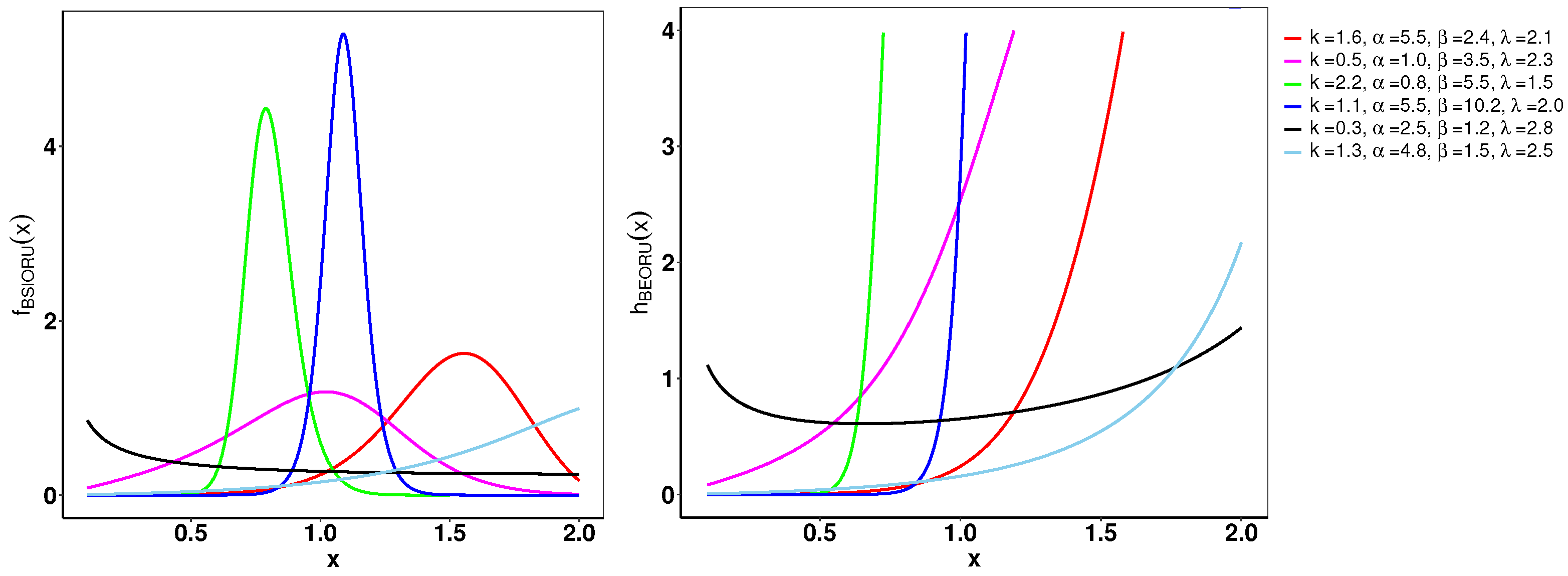
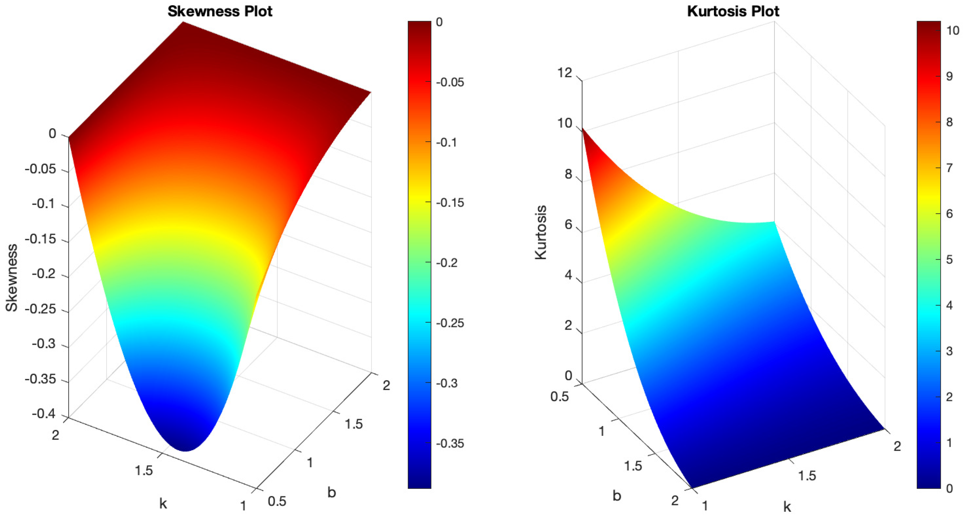
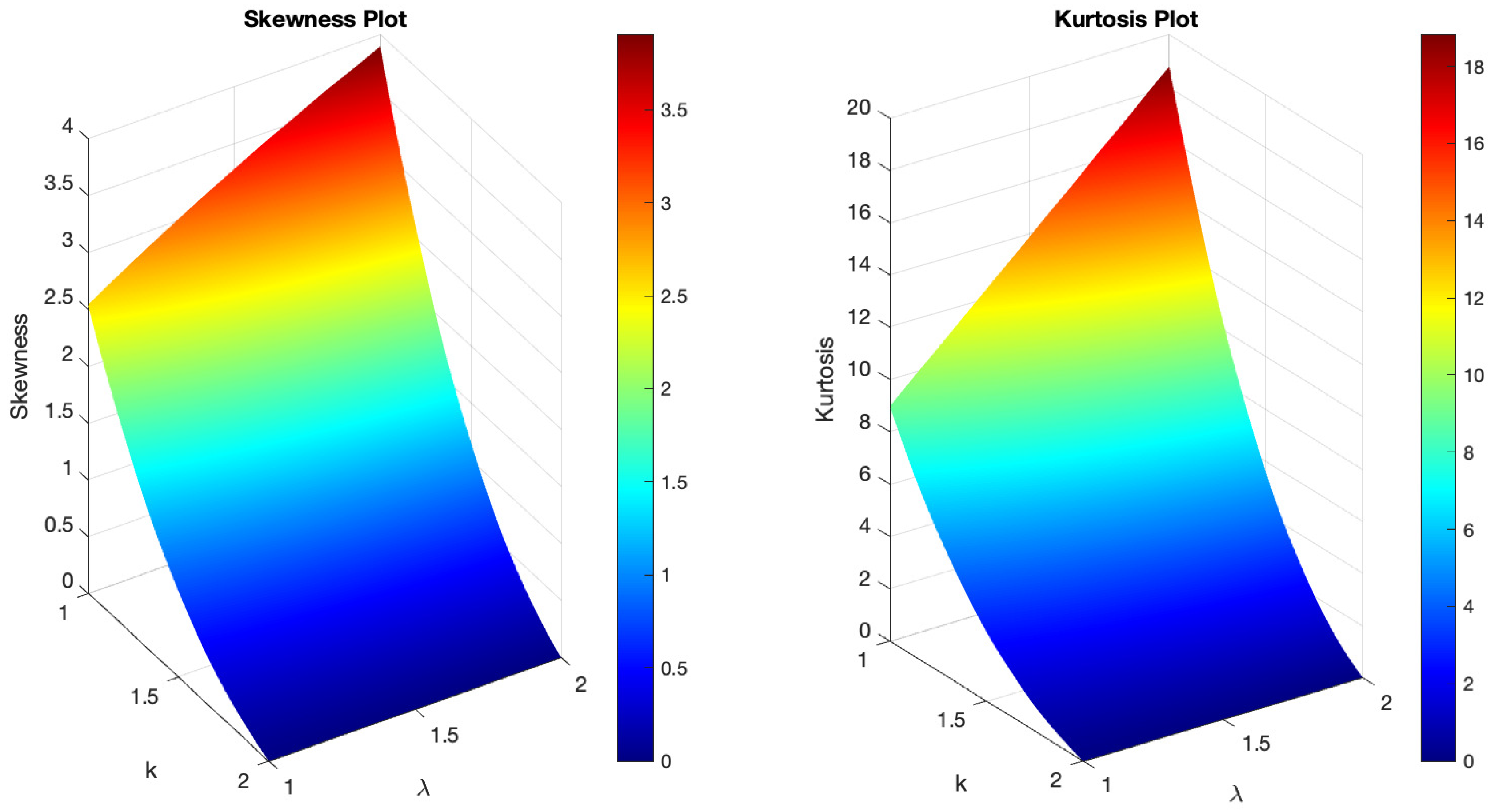
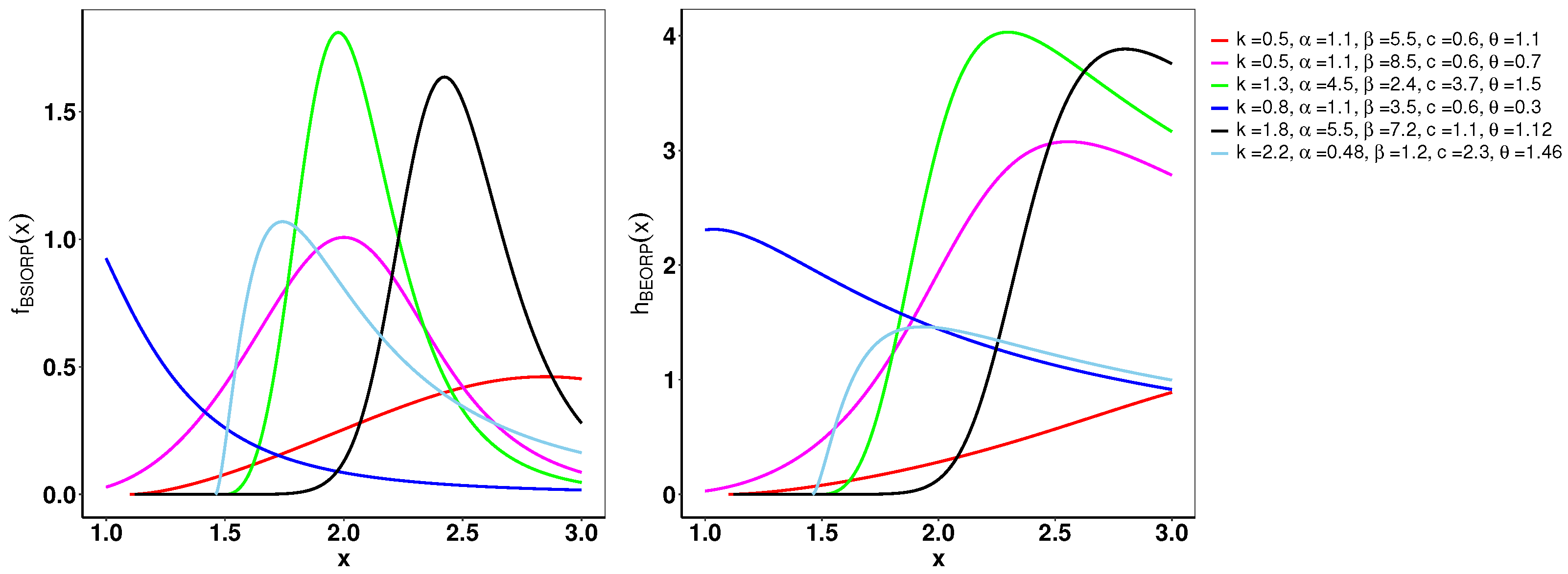
Figure 1 demonstrates the variability of the B-SIOR-U distribution in augmenting the baseline function of the uniform distribution. The pdf exhibits a range of shapes including symmetric, left- and right-skewed, J-shaped, and inverse-J shaped. Similarly, the hrf displays varying patterns, including different patterns of increasing and bathtub shapes. Skewness and kurtosis plots for the B-SIOR-U distribution, based on specific parameter selections, are depicted in Figure 2 and Figure 3, respectively. Additional skewness and kurtosis plots, exploring a wider array of parameter combinations, are available in the Supplementary Information. These extended visualizations offer deep insights into how the B-SIOR-U distribution’s characteristics evolve with different parameter values.
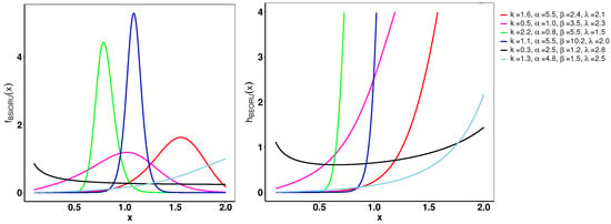
Figure 1.
Plots of the pdf (left) and hrf (right) for the B-SIOR-U distribution with chosen parameter values. We denote as the input vector for these functions, where .
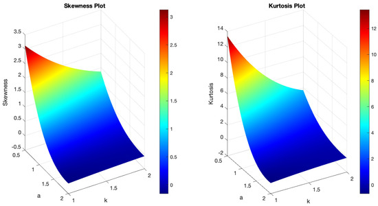
Figure 2.
(Left) The skewness plot of B-SIOR-U . (Right) The kurtosis plot of B-SIOR-U .

Figure 3.
(Left) The skewness plot of B-SIOR-U . (Right) The kurtosis plot of B-SIOR-U .
3.2. Burr III Scaled Inverse Odds Ratio–Exponential Distribution
We consider the exponential distribution as the baseline , characterized by a positive parameter , whose pdf and cdf are and , respectively.
The cdf for the Burr III Scaled Inverse Odds Ratio–Exponential (B-SIOR-E) distribution is formulated as
and the pdf is
with , , and .
The hrf for the B-SIOR-E distribution is given by
and the reverse hrf is
The quantile function, derived from solving , is expressed as
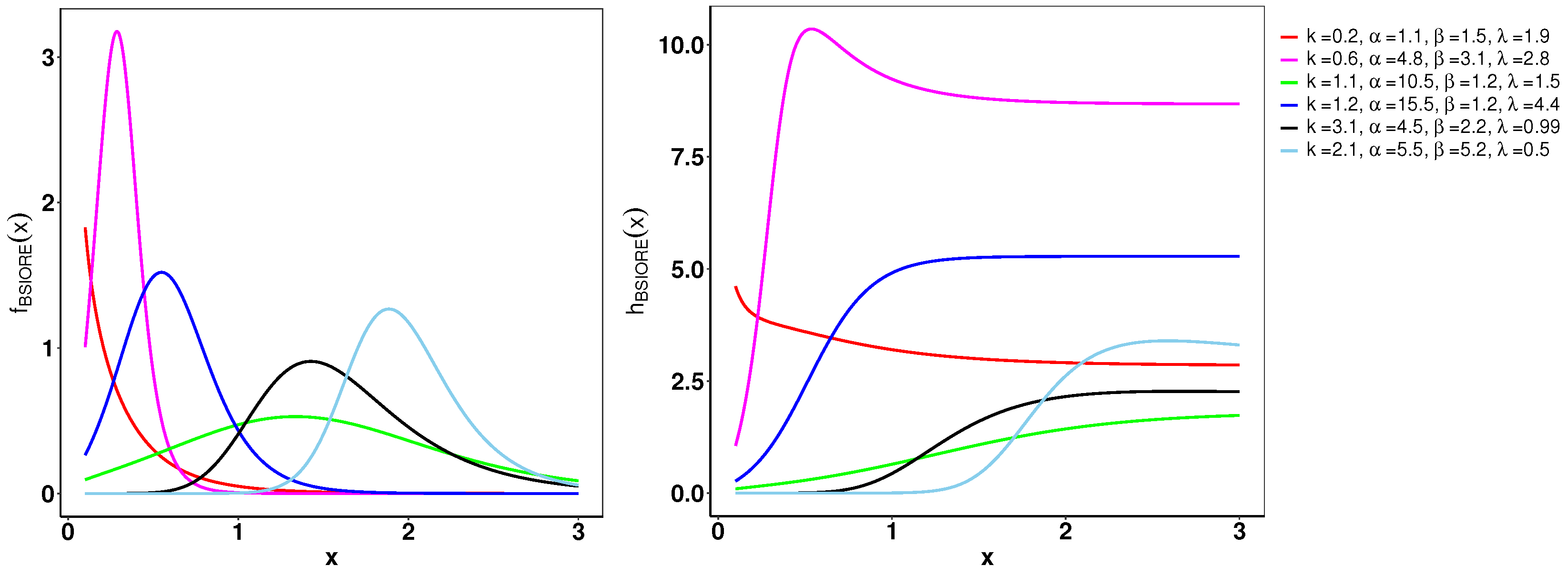
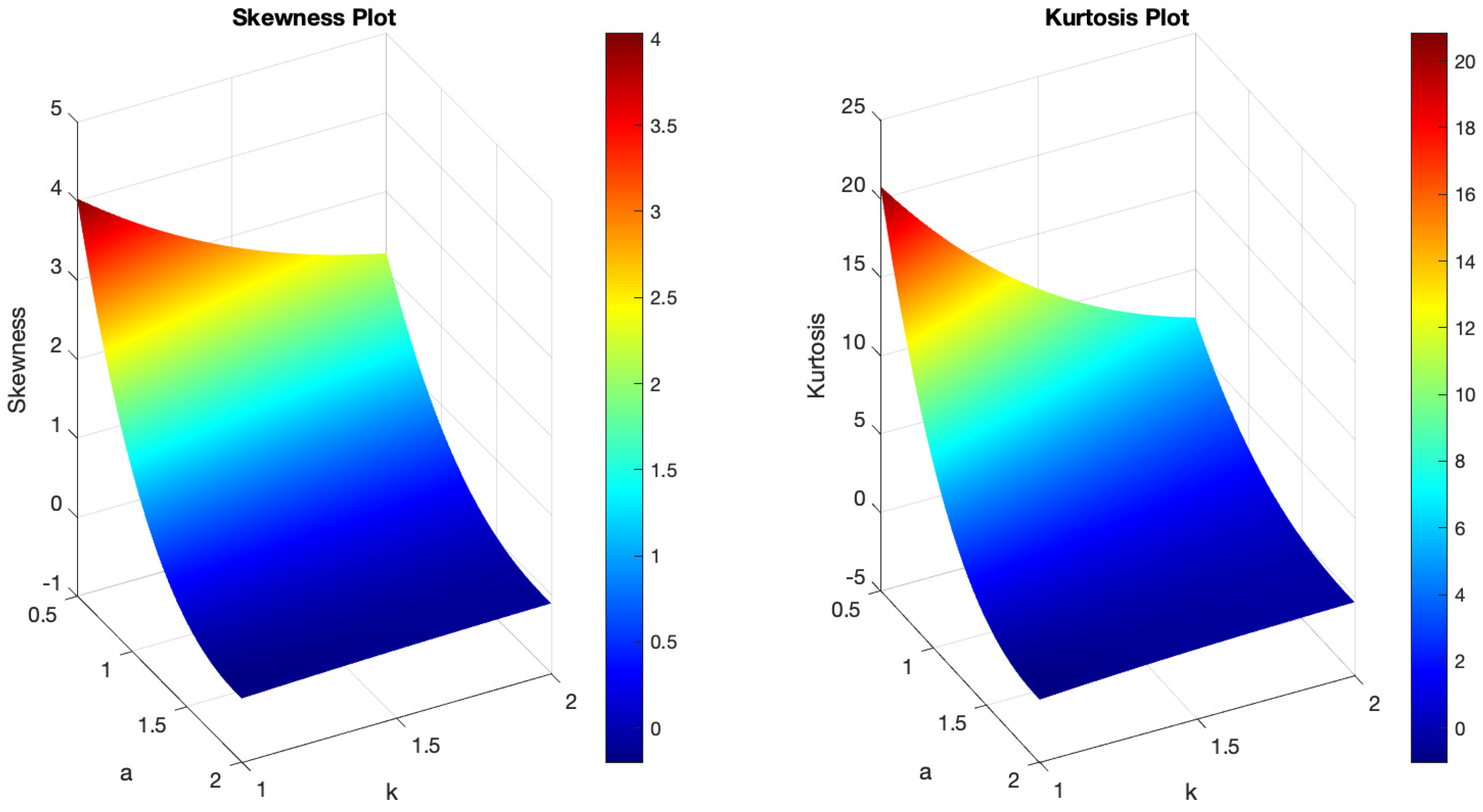
Example plots illustrating the pdf and hrf of the B-SIOR-E distribution, for selected parameter values, are shown in Figure 4. Originating from the exponential distribution’s inherently monotonically decreasing pdf, the B-SIOR-E model is capable of transforming this into diverse shapes, including left-skewed, right-skewed, decreasing, and near-symmetric configurations. Similarly, the hrf exhibits a variety of forms, encompassing increasing, decreasing, and upside-down behaviorshaped patterns, illustrating the adaptability of the B-SIOR-E distribution in modeling different types of data behavior. Additionally, the skewness and kurtosis plots for the B-SIOR-E distribution, featuring selected parameter values, are displayed in Figure 5 and Figure 6, respectively. Detailed plots showcasing various skewness and kurtosis values across different parameter combinations are included in the Supplementary Materials for comprehensive analysis and insight.

Figure 4.
The left and right of the figure are the pdf and cdf of the B-SIOR-E distribution for various parameter settings, resepectively.

Figure 5.
(Left) The skewness plot of B-SIOR-E . (Right) The kurtosis plot of B-SIOR-E.

Figure 6.
(Left) The skewness plot of B-SIOR-E . (Right) The kurtosis plot of B-SIOR-E.
3.3. Burr III Scaled Inverse Odds Ratio–Pareto Distribution
We consider the baseline distribution as a Pareto distribution characterized by two positive parameters and . Consequently, the pdf of the Pareto distribution is denoted by , and its cdf by .
The cdf of the Burr III Scaled Inverse Odds Ratio–Pareto (B-SIOR-P) distribution is defined as
and the pdf is articulated as
where , , and .
The hrf for the B-SIOR-P distribution is expressed as
and the reverse hrf is given by
Moreover, by solving the equation , the quantile function is derived as follows
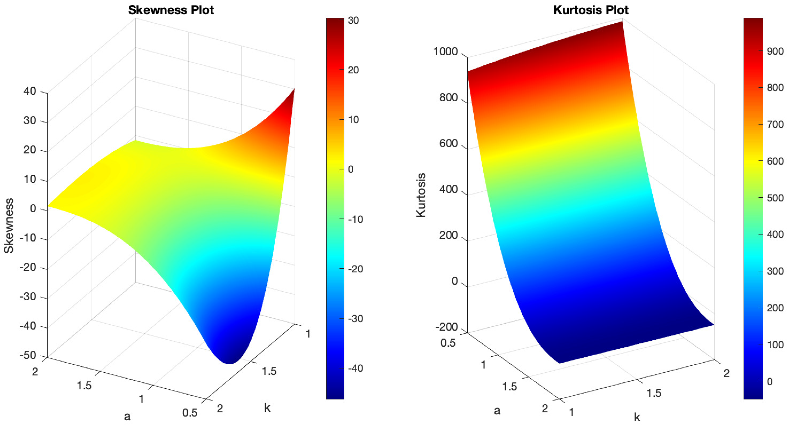
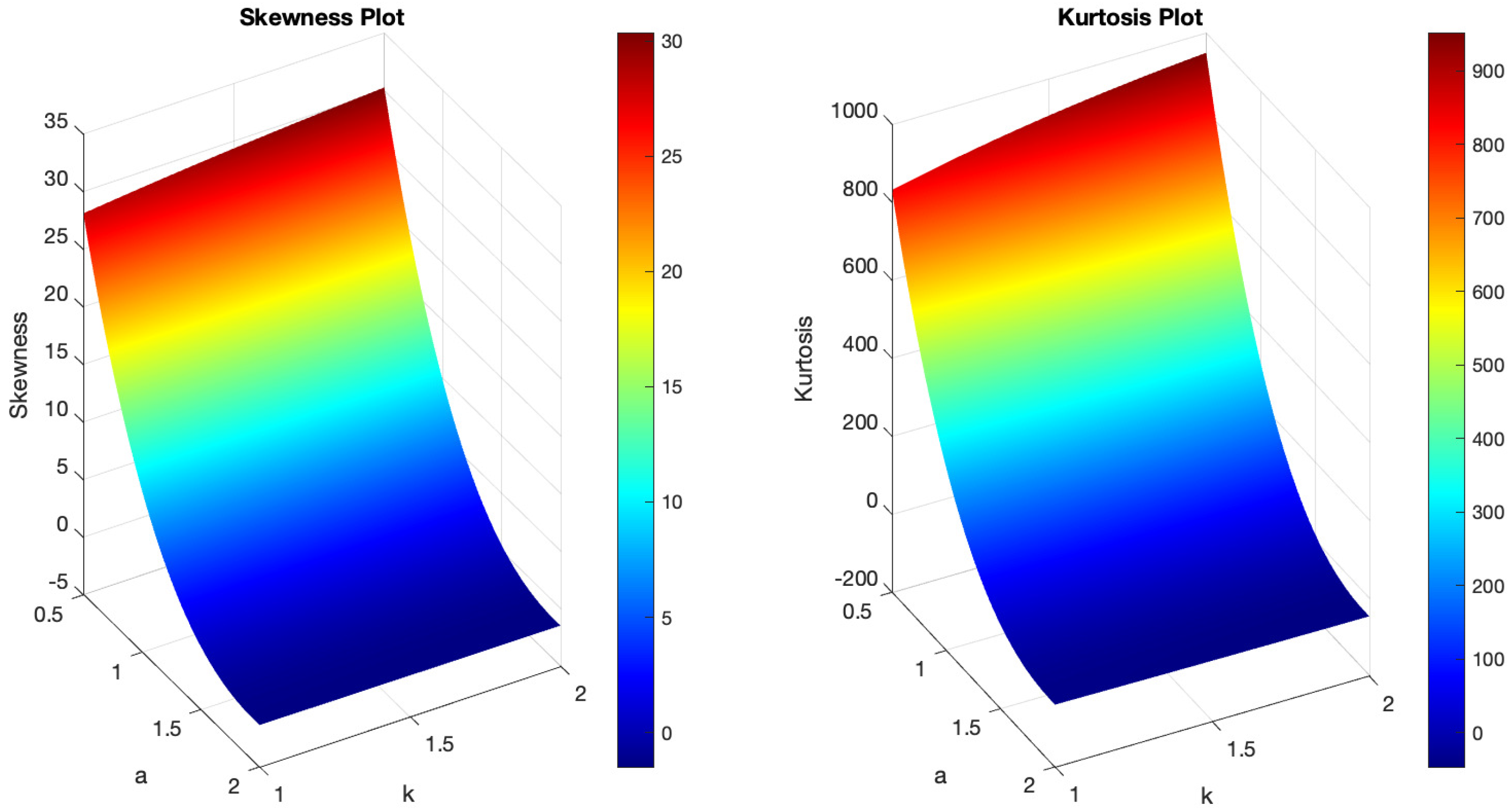
As illustrated in Figure 7, the pdf of the B-SIOR-P distribution can exhibit various shapes including decreasing, increasing, left- and right-skewed, as well as almost symmetric patterns. Similarly, the hazard rate function of the B-SIOR-P distribution can manifest in increasing, decreasing, stretched S, and inverted U shapes. Figure 8 and Figure 9 depict the skewness and kurtosis for the B-SIOR-P distribution under specific conditions. Additional plots of skewness and kurtosis for the B-SIOR-P distribution with various parameter settings are available in the Supplementary Materials, providing further insights into the distribution’s behavior across different parameter values.
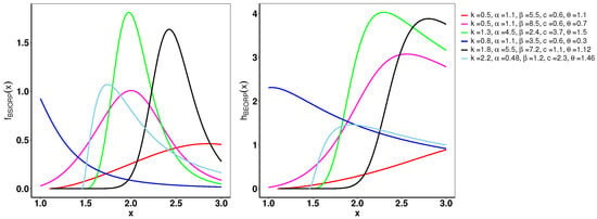
Figure 7.
On the left, the pdf of the B-SIOR-P distribution for various parameters is depicted. On the right, the hrf of the B-SIOR-P distribution for different parameter configurations is illustrated.

Figure 8.
(Left) The skewness plot of B-SIOR-P . (Right) The kurtosis plot of B-SIOR-P .

Figure 9.
(Left) The skewness plot of B-SIOR-P . (Right) The kurtosis plot of B-SIOR-P .
The three special cases presented above demonstrate the adaptability and diversity of the new B-SIOR-G family of distributions. Both the cdf and the quantile functions possess relatively simple formats, which facilitate easier and more reliable statistical inferences. The transformations applied to single-parameter distributions further validate the effectiveness of this new model, showcasing its robust potential for modeling diverse types of data.
4. Statistical Properties of the Burr III Scaled Inverse Odds Ratio–G Distribution
Given the extensive formulation of the probability density function in Equation (3), computing the statistical properties of this new family of distributions could involve intricate processes, and deriving closed forms for complex parent distributions may be challenging. To expedite these calculations, we will first expand the pdf of the B-SIOR-G into the well-known exponentiated-G distribution, for which the statistical properties have been established both theoretically and numerically. This expansion simplifies the computation of all related statistical measures, including moments, the moment-generating function, incomplete and conditional moments, moment of residual life and reversed residual life, the Rényi entropy, order statistics, stochastic ordering, and probability-weighted moments. Due to the complexity of this paper, comprehensive proofs and detailed derivations of these properties are provided in the Supplementary Information, accessible at https://github.com/shusenpu/B-SIOR-G/blob/main/Supplementary_Info.pdf (accessed on 2 May 2024).
4.1. Basic Properties of the B-SIOR-G Distribution
A series of expansions for the probability density function allows for simplifying calculations in properties’ derivations, approximating functions during simulation processes, and facilitating the analytical manipulation of the pdf.
Theorem 1.
The pdf of the B-SIOR-G distribution can be expressed as a linear combination of the exponentiated generalized distribution as follows:
where the coefficients are given by
and the term is defined as
representing the exponentiated generalized distribution’s pdf given parameter .
Proof.
We consider the general form of binomial series expansion:
Thus, the pdf of the B-SIOR-G distribution can be expanded as
We note that, using the definition of odds ratio, the function can be generalized as
Therefore, we have the pdf as
where
and
which is the pdf of the exponentiated generalized distribution with parameter . □
The pdf is represented as an infinite series, which implies that the function can be approximated by sufficiently summing many terms of the series to approximate its true value. The quality of the approximation typically improves as more terms are included. The coefficients modify the contribution of each term in the series. These coefficients can be interpreted as weights that adjust the influence of each term based on the distribution. It can be easily demonstrated that the series converges because it forms a geometric sequence with a common ratio . The expansion provides an intuitive and easier way to calculate the statistical properties of the distribution, while it is relatively difficult to perform derivations like integration on the original pdf with odds ratios.
The hrf defines the instantaneous rate at which events occur, given that no prior event has happened. A higher hazard rate at a certain time indicates a greater risk of the event happening. The hazard rate does not represent the probability of an event occurring at a specific time but the rate or intensity of occurrence at an infinitesimal interval around that time. In their seminal work, ref. [33] demonstrated the equivalent behavior of hrf, reverse hazard function and the mean residual life function.
Remark 1.
The hrf of the distribution can be derived as follows:
and the reverse hrf is
The quantile function, which can also be termed as the inverse cdf, serves as a method to map probabilities back to values in the domain of a random variable. For a given probability p (where ), the quantile function provides the value x such that the probability of the random variable being less than or equal to x is p.
Remark 2.
The quantile function for the B-SIOR-G distribution is defined as
where and
Generally, the quantile function can be used to find percentiles and could be used for inferences. For example, gives the median of the distribution, the value below which of the data falls. The simple form of the quantile function q provides a direct way to calculate the probability since it can be solved directly by plugging in the quantile values.
4.2. Moments, Incomplete Moments, and Generating Functions
Moments serve as statistical indicators that succinctly capture the essence of probability distributions and datasets.
Remark 3.
For a random variable Y∼, the rth moment of the B-SIOR-G distribution is
where follows the exponentiated generalized distribution, which is obtained by raising the cdf of a baseline distribution to a certain power, with as defined in Theorem 1.
The convergence of the rth moment can be demonstrated by examining the expansion of the pdf of B-SIOR-G, where the pdf can be expressed as a coefficient multiplied by a certain power of the parent cdf, . On one end, as i and j increase, the tails of the power series approach zero since . On the other end, the powers of can be sorted while calculating the rth moment of . To establish an upper bound for , we replace all coefficients with their maximum value and rank the according to the power of , forming a geometric series with a common ratio of . Therefore, we conclude that converges. A similar approach can be applied to demonstrate that the infinite series converges in all remaining conclusions and remarks.
An incomplete moment refers to the moment of a portion of a distribution. It is defined as the expected value of a given function of a random variable over a specified range, which is in contrast to the complete moment that takes into account the entire distribution.
Remark 4.
The incomplete moment for the distribution is formulated as
where is the incomplete moments of the exponentiated-G distribution. Here, we can examine the moment in the designated range from 0 to z as specified by the range, which is especially useful when dealing with truncated proportions of distribution, such as censoring in survival analysis.
The moment generating function (mgf) encapsulates all the moments of the probability distribution. By evaluating its derivatives at zero, the mgf provides a systematic way to calculate the mean, variance, skewness, and other moments of the distribution.
Remark 5.
The mgf can be found using
where denotes the mgf of the exponentiated generalized distribution with parameter .
Thus, the overall distribution is a mixture or combination of multiple distributions, each with a different parameter . Adjusted by the coefficient weights , each contributes to the overall , which can be used for finding the n-th moment of the distribution by taking the n-th derivative of the resulting function.
4.3. Moment of Residual Life and Reversed Residual Life
In survival analysis and reliability engineering, the moment of residual life and moment of reversed residual life are essential for analyzing the distribution of time-to-event data. The moment of residual life at the time t quantifies the expected remaining lifetime given that an event has not occurred by t. Conversely, the moment of reversed residual life at the time t reflects the expected past duration given that an event occurred before t.
Lemma 1.
The moment of residual life, denoted as , is formally defined as
where X is the lifetime random variable, and m is the moment order. The moment of residual life of the distribution can be derived from Equation (10):
where is the pdf of exponentiated-G with parameter .
Following a similar calculation, we can find the mth moment of reversed residual life as follows.
Remark 6.
The moment of reversed residual life, denoted as , can be derived as
4.4. Skewness and Kurtosis Analysis
Skewness quantifies the asymmetry of the distribution, while kurtosis measures its tail heaviness, with positive skewness indicating a right-skewed distribution and kurtosis indicating peakedness.
Lemma 1.
Given , the coefficient of skewness () for Y∼ is
and the coefficient of kurtosis () is
4.5. Rényi Entropy
Rényi entropy is a generalization of the Shannon entropy and provides a measure of the diversity, uncertainty, or randomness of a probability distribution.
Theorem 2.
The Rényi entropy for the B-SIOR-G distribution is calculated as
where , indicating the diversity of values the distribution can take, with being the Rényi entropy for the exponentiated generalized distribution parameterized by .
Proof.
The Rényi entropy of the B-SIOR-G distribution is given by
where and . By applying the same expansion technique for the pdf, we obtain
Using the definition of odds ratio, we have
Therefore, the further expansion of the Rényi entropy can be generalized as
where is the Rényi entropy of the exponentiated generalized distribution with parameter . □
The Rényi entropy for the B-SIOR-G distribution captures the diversity of the distribution’s outcomes weighted by the order . Higher values of indicate greater uncertainty or randomness within the distribution for the given order .
4.6. Order Statistics and Stochastic Ordering
Theorem 3.
For as i.i.d. random variables from the B-SIOR-G distribution, the pdf of the jth order statistic is
expressing as a linear combination of B-SIOR-G with parameters , where .
Proof.
Let be independent identically distributed random variables distributed by the B-SIOR-G distribution. The pdf of the jth order statistic is given by
□
Theorem 4.
Given ∼ and ∼, the likelihood ratio Λ is
indicating the relative likelihood of outcomes from two distributions based on their parameters.
Earlier order statistics (smaller j) tend to have “lighter” tails as they are biased towards smaller values, whereas later order statistics (larger j) have “heavier” tails, reflecting larger sample values. The parameter modification implies that higher-order statistics or terms in the sum increasingly stretch or scale the distribution, accounting for the more extreme values expected in higher-order statistics.
4.7. Probability Weighted Moments
Probability Weighted Moments (PWMs) are derived from our probability distribution, which weights moments by the probabilities themselves. They provide a way to summarize the shape of a probability distribution and are particularly useful for characterizing the tails of the distribution.
Lemma 4.
The rth PWM for the distribution can be calculated as follows:
which simplifies to
for non-negative integers p, q, and r. For practical applications, often, ; thus, the PWM simplifies further, to
A common example used for illustration is the first PWM (), expressed as
for and , which simplifies the evaluation process for specific cases.
Commonly, in practice, particularly for hydrological models where one might want to understand the mean behavior rather than moments of higher order, r is set to 0, simplifying the PWM to only consider the probability weights without raising x to any power.
5. Methods of Estimation
In this section, we discuss five estimation methods crucial for discerning the parameters of proposed B-SIOR-G distributions. The exploration of these methods is the key to achieving accurate approximations that align B-SIOR-G models with observed data. Then, we apply the Monte Carlo simulation to test the convergence of approximated parameters as the sample sizes grow to determine its reliability. The estimation methods include the Maximum Likelihood Estimation (MLE), Least Square (LS) and Weighted Least Square (WLS) Estimation, Maximum Product Spacing Estimation (MPS), the Cramér–von Mises Estimation (CVM), and the Anderson and Darling Estimation (ADE).
Given an independent random sample from the B-SIOR-G distribution with parameter vector , the likelihood function is formulated as
MLE seeks to find the set of parameters that maximize the likelihood function, making it a powerful method for parameter estimation by leveraging the full probability model, as shown in Equation (11).
The LS technique in Equation (12) minimizes the sum of the squared differences between observed and theoretical values, offering a straightforward approach for fitting models to data by emphasizing overall error reduction. An extension of LS, from Equ ation (13), WLS, assigns weights to data points, prioritizing certain observations over others, thus refining the fitting process, especially when dealing with heteroscedastic data. The LS and WLS methods are expressed as [34]
and
Both methods aim to find the best parameters () that align the theoretical distribution specified by the B-SIOR-G model as closely as possible to the observed data.
The MPS is valuable for complex distributions, as highlighted by Cheng and Amin [35]. The MPS is maximized by optimizing
where represents spacing functions and estimators are found by solving . MPS in Equation (14) focuses on maximizing the product of the spacings between ordered observations and their estimated distribution, providing an alternative to MLE that is less sensitive to outliers.
Estimators are derived by minimizing the Cramér–von Mises criterion, , with respect to , where
The Cramér–von Mises distance between continuous distribution functions is one of the distinguished measures of deviation between distributions, as shown in Equation (15).
As an advancement of the Cramér–von Mises criterion, the Anderson–Darling approach in Equation (16) places more weight on the tails of the distribution, making it particularly useful for detecting discrepancies in the distribution’s extremities. By minimizing the formula below, we can obtain the Anderson–Darling estimators:
This method emphasizes the tails of the distribution, making it particularly useful for distributions with significant tail behaviors.
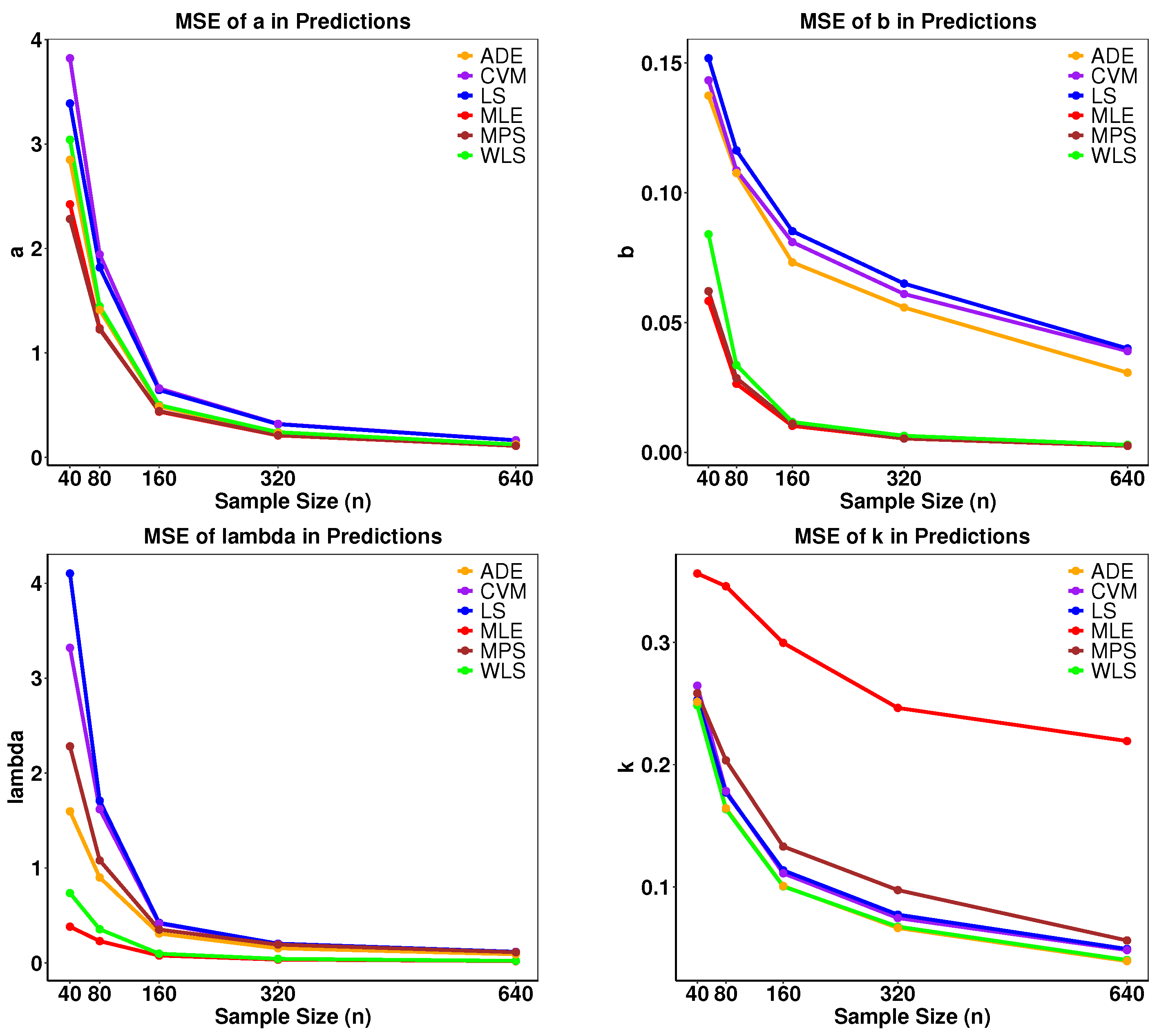
To determine the maximum or minimum values of each estimator, we differentiate the specified objective functions and use numerical methods such as iteratively reweighted least squares (IRLS) or Newton–Raphson to locate their extreme values. For a practical demonstration of how the numerical simulation operates, we employ B-SIOR-E as an illustrative example. The detailed steps of the simulation process are outlined in Algorithm 1. We conducted a comprehensive simulation study using Monte Carlo simulations to estimate the parameters of the B-SIOR-E distribution. Then, we picked , , , and as the initial values for each parameter. Please note that the model is highly nonlinear and sensitive to the initial parameter values. Then, , 80, 160, 320, and 640 were selected as sample sizes to generate random samples, with each experiment replicated 500 times to ensure statistical reliability. The resulting data were then analyzed to compute both bias and mean squared error (MSE) for each dataset. As illustrated in Figure 10, the MSE demonstrated convergence towards 0 with increasing N, affirming the stability and reliability of the estimations across all cases.
| Algorithm 1 Monte Carlo Simulation for Parameter Estimation |
|
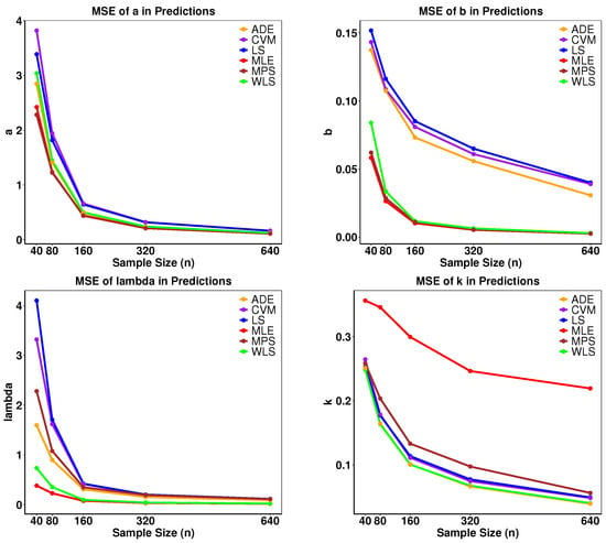
Figure 10.
Mean squared error of parameters estimations for different methods.
6. Application
In this section, we transition from theoretical discussions to practical examinations, highlighting the applicability of our model through the analysis of real-world datasets. This exploration is designed to validate the practical utility of the newly introduced B-SIOR-U and B-SIOR-E distributions by showcasing their effectiveness in real data-driven scenarios. Some simple and well-known distributions such as gamma, generalized exponential, Log-logistic, and Weibull distributions are included in the comparison. Given that the B-SIOR-E model derives from the Burr III and exponential distributions, we aim to benchmark it against other models based on Burr III [5], as well as those related to the Weibull and exponential distributions—Weibull generalized exponential (WGE) distribution [26], known for its applicability in complex scenarios. Furthermore, in light of Chen’s work [25] on Type-2 Gumbel distributions, we have also incorporated comparisons with Type-2 Gumbel (T2G) [27], Lomax Gumbel Type-2 (LGT) [28], and Exponentiated Generalized Gumbel Type-2 (EGG2) distributions [29] into our analysis. It should be noted that both LGT and EGG2 have four parameters each. When these models are compared to B-SIOR-E and B-SIOR-U, the significance of the proposed model is evident, even though it shares the same number of parameters with its counterparts.
To thoroughly assess and compare the efficacy of statistical models, several goodness-of-fit metrics were employed, each evaluating distinct facets of model performance. The metrics include the following:
- The -2 Log-Likelihood Statistic [36], which quantifies the fit of a model by summarizing the discrepancies between observed and expected values under the model. A lower statistic suggests a better fit and this metric underpins various other statistical tests.
- Cramér–von Mises Statistic () [37], which measures how closely a theoretical cdf matches the empirical cdf by integrating the squared differences across all values. A lower value indicates a better fit, as it means there is less deviation between the theoretical and empirical cdfs. This provides a thorough assessment of the deviation between the modeled and observed data.
- Anderson–Darling Statistic () [38], akin to but placing greater emphasis on the tails of the distribution. This makes it particularly sensitive to extremities in data, valuable for analyses where tail behavior is crucial. A lower value indicates a better fit, especially when the tails of the distribution are well modeled.
- Akaike Information Criterion () [36], which balances model fit against the number of parameters, penalizing unnecessary complexity. Derived from information entropy, it seeks to minimize information loss, preferring models with lower values. A lower value indicates a better fit, as it suggests that the model achieves a good balance between accuracy and simplicity.
- Bayesian Information Criterion () [39], similar to but imposing a stronger penalty on the number of parameters. Based on Bayesian probability, it is useful for selecting among a finite set of models, favoring simplicity unless a more complex model significantly enhances fit. A lower value indicates a better fit, favoring models that are simpler and have fewer parameters unless a more complex model significantly improves the fit.
- Consistent Akaike Information Criterion () [40], an augmentation of that incorporates an extra penalty for parameter count, making it more conservative and particularly apt for larger datasets where overfitting is a concern. A lower value indicates a better fit, particularly in larger datasets where it helps avoid overfitting.
- Hannan–Quinn Criterion () [41], which, like and , employs a logarithmically growing penalty term with sample size. It offers a compromise between the propensity of to overfit and the strict penalties of . A lower value indicates a better fit, balancing between the risk of overfitting and underfitting.
- Kolmogorov–Smirnov Test Statistic () [42], which identifies the maximum divergence between the empirical distribution function of the sample and the cumulative distribution function of the reference distribution. The corresponding p-value assists in recognizing statistically significant deviations, with a smaller statistic indicating a more accurate fit between observed and modeled distributions, as it suggests minimal divergence.
6.1. Lifetime Data
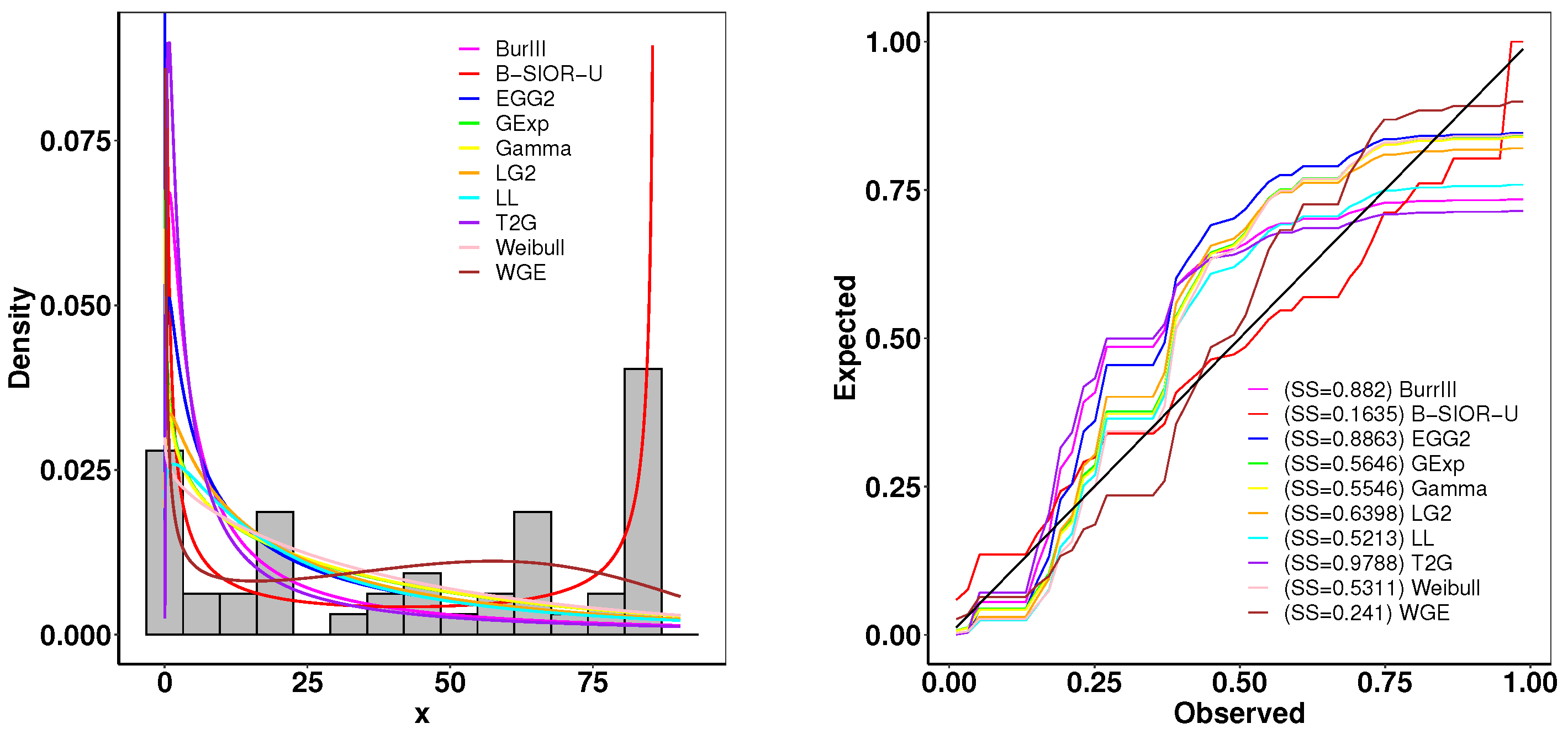
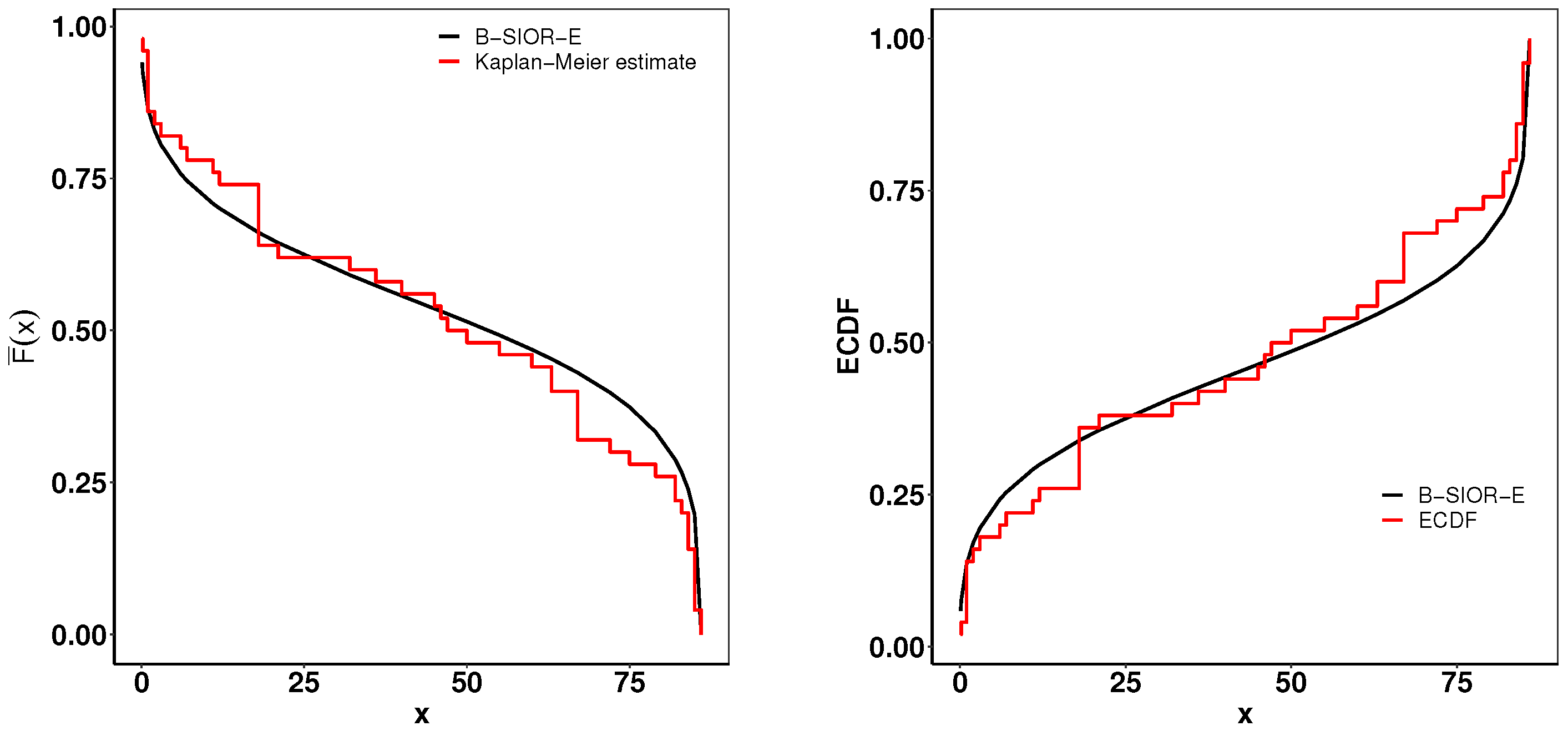
The first dataset contains the lifetime data of 50 devices, which was provided in [43]. The goodness-of-fit statistics are shown in Table 1 and Figure 11 presents the histogram of observed data and the density plots of fitted distributions. The B-SIOR-U distribution emerges as the best model for this bathtub dataset since it has the optimal goodness-of-fit metrics and the highest K-S test p-value. Figure 12 illustrates the Kaplan–Meier (K-M) survival curve and both theoretical and empirical cdfs. The theoretical predictions align well with actual data, highlighting that the B-SIOR-U distribution is effective in modeling the data with a bathtub shape.

Table 1.
Parameter estimates and goodness-of-fit statistics for lifetime data.
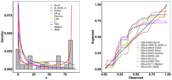
Figure 11.
(left) Fitted density and histogram. (right) Observed and expected probability plots.

Figure 12.
(left) Fitted Kaplan–Meier survival curve. (right) Theoretical and expected CDFs.
6.2. Failure Data
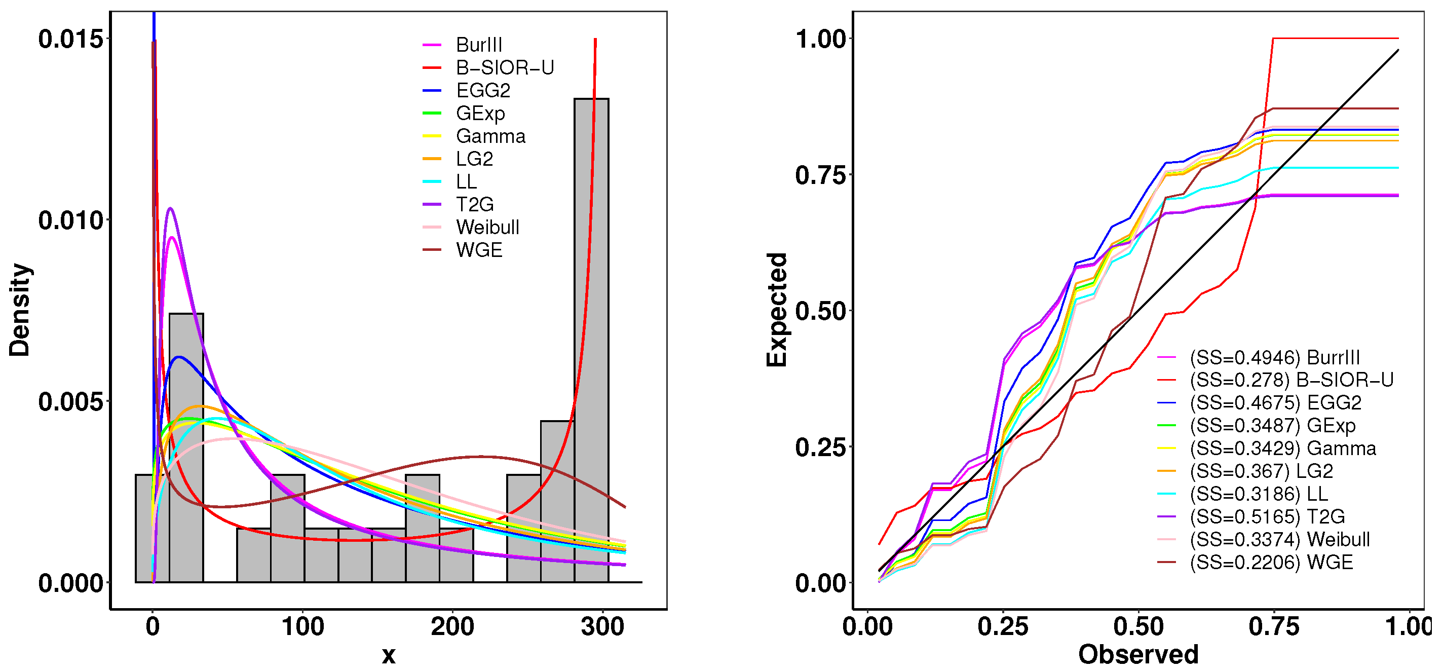
This dataset contains the failure and running times of a sample of 30 devices given by Meeker and Escobar [44]. The model results are shown in Table 2. Figure 13 presents the histogram of observed data and the density plots of fitted distributions. The B-SIOR-U distribution has the best performance for this dataset since it has the optimal value of all goodness-of-fit metrics. Figure 14 presents the Kaplan–Meier (K-M) survival curve and the theoretical and empirical cdfs plot. It is obvious that the B-SIOR-U distribution can approximate the true data well.

Table 2.
Parameter estimates and goodness-of-fit statistics for failure data.
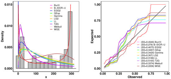
Figure 13.
(left) Fitted density and histogram. (right) Observed and expected probability plots.
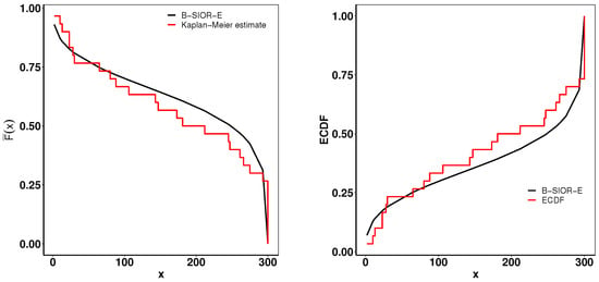
Figure 14.
(left) Fitted Kaplan–Meier survival curve. (right) Theoretical and expected CDFs.
6.3. Lung Cancer Data
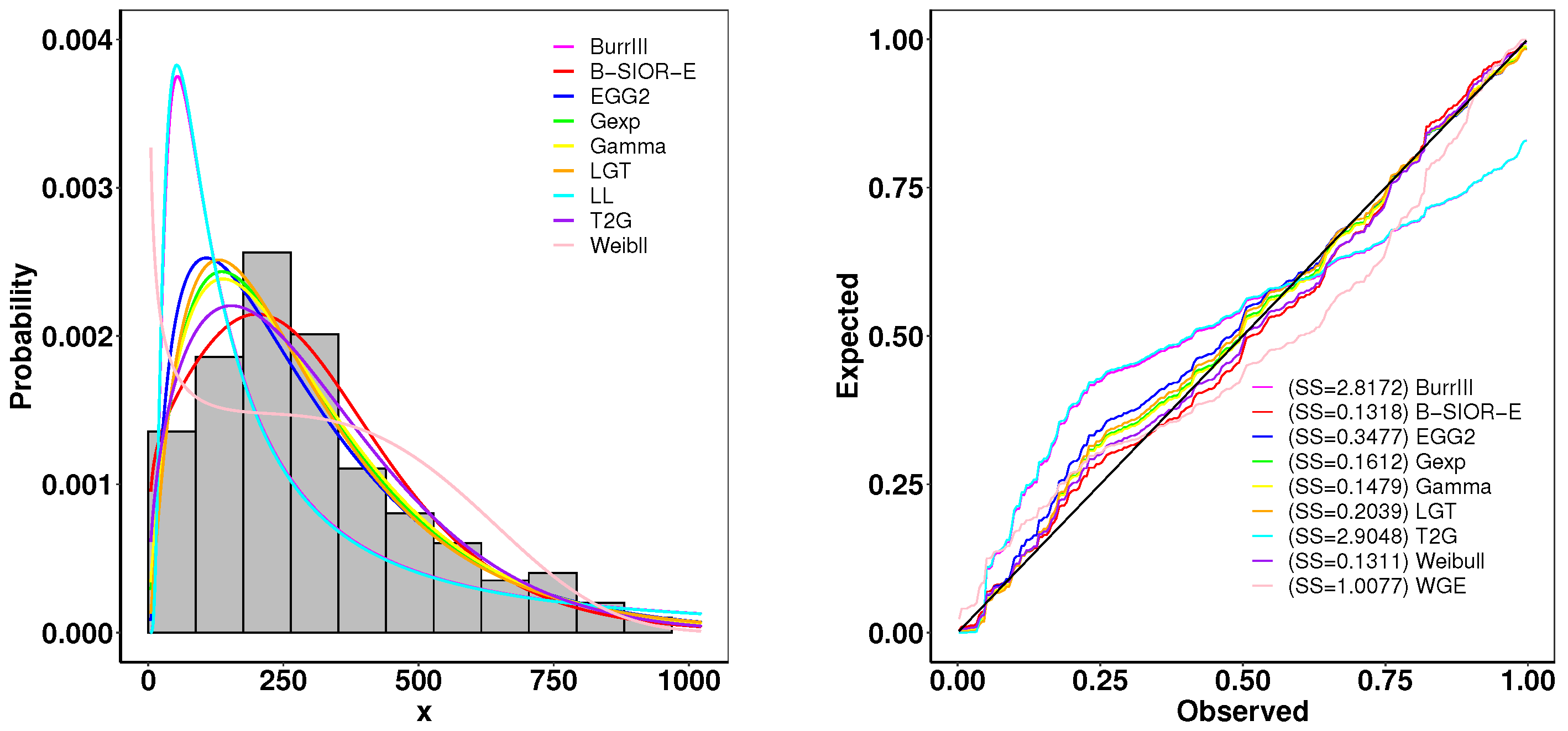
This dataset contains the survival time of 128 patients with advanced lung cancer from the North Central Cancer Treatment Group. A summary of parameter estimates and goodness-of-fit metrics is presented in Table 3, while Figure 15 illustrates the comparison between the histogram of observed data and the density plots of fitted distributions. The B-SIOR-E distribution emerges as the superior model for this dataset, evidenced by its better goodness-of-fit metrics and the highest K-S test p-value, as detailed in Table 3.

Table 3.
Parameter estimates and goodness-of-fit statistics for lung cancer data.
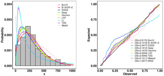
Figure 15.
(left) Fitted density and histogram. (right) Observed and expected probability plots.
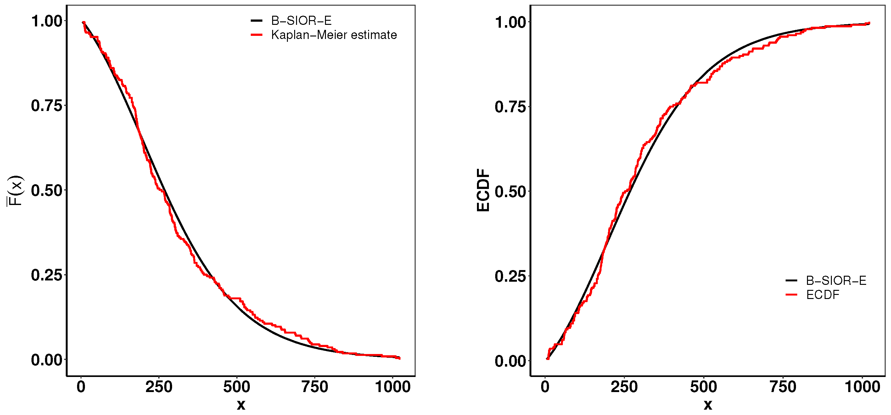
Figure 16 presents a suite of plots including the Kaplan–Meier (K-M) survival curve, both theoretical and empirical cdfs, and a Total Time on Test (TTT) plot adjusted for scaling. The empirical consistency observed between theoretical predictions and actual data underscores the B-SIOR-E distribution’s adeptness at modeling the data with a monotonic hazard rate structure.
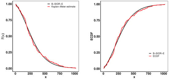
Figure 16.
(left) Fitted Kaplan–Meier survival curve. (right) Theoretical and expected CDFs.
6.4. Bladder Cancer Data
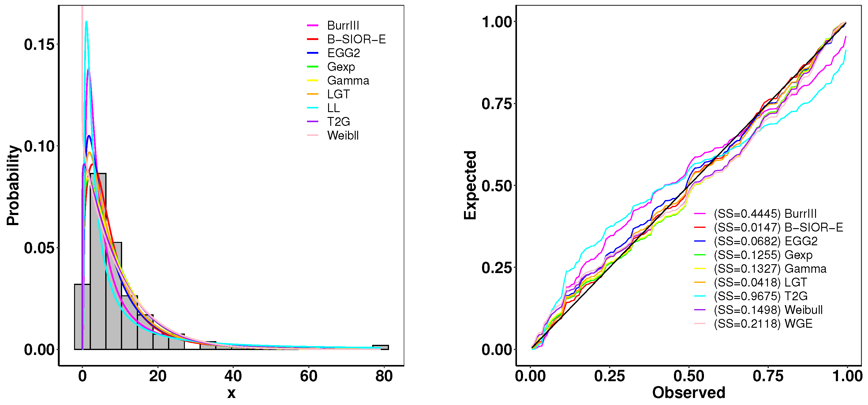
This dataset represents the recorded remission times given in months from bladder cancer patients, reported by Lee and Wang [45]. A summary of parameter estimates and goodness-of-fit metrics is presented in Table 4, while Figure 17 illustrates the comparison between the histogram of observed data and the density plots of fitted distributions. The B-SIOR-E distribution emerges as the superior model for this dataset, evidenced by its better goodness-of-fit metrics and the highest K-S test p-value, as detailed in Table 4.

Table 4.
Parameter estimates and goodness-of-fit statistics for bladder cancer data.
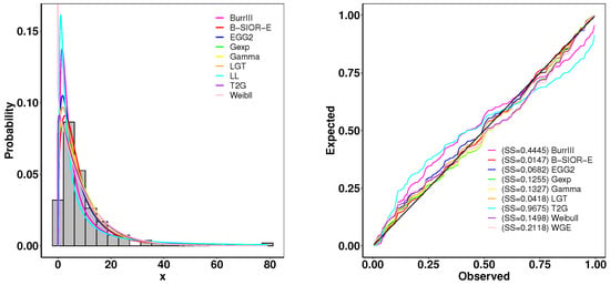
Figure 17.
(left) Fitted density and histogram. (right) Observed and expected probability plots.
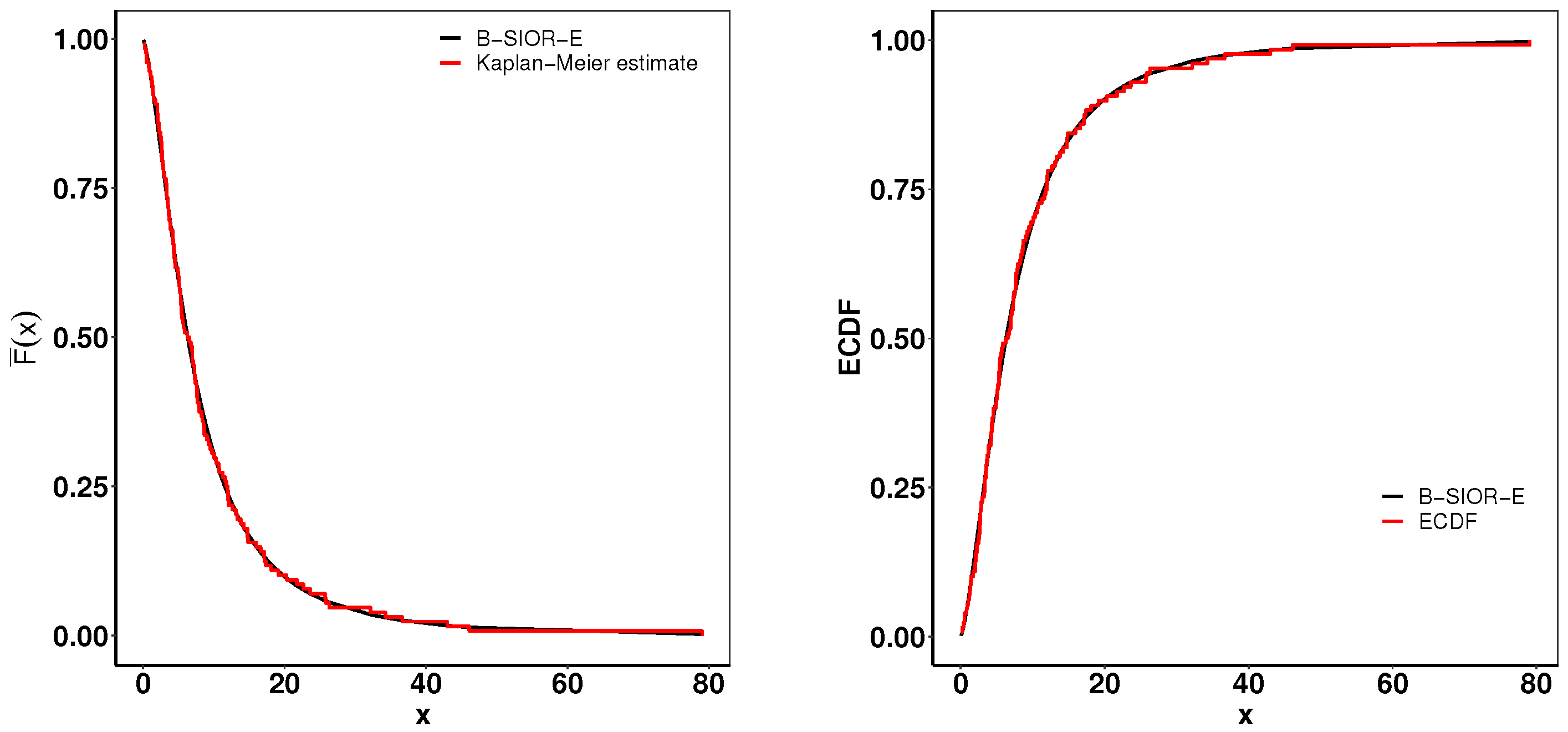
Figure 18 presents a suite of plots including the K-M survival curve, both theoretical and empirical cdfs, and a TTT plot adjusted for scaling. The empirical consistency observed between theoretical predictions and actual data underscores the B-SIOR-E distribution’s adeptness at modeling the data with a monotonic hazard rate structure.
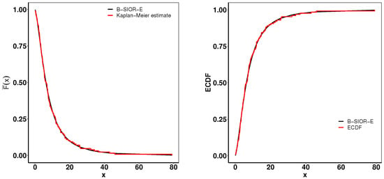
Figure 18.
(left) Fitted K-M survival curve. (right) Theoretical and expected cdfs.
These results from real-world datasets do more than just confirm the statistical robustness of the B-SIOR-G model; they also amplify its practical relevance in the field of biomedical science. By accurately capturing the dynamics of the specified cancer datasets, this method supports predictive maintenance and ensures the quality of materials essential for advanced applications. The successful correlation of theoretical models with empirical evidence highlights the model’s capability to enhance decision-making in healthcare. The primary contribution of the proposed family of distributions lies in its exceptional performance in modeling bathtub-shaped data. While traditional distributions such as gamma, generalized exponential, Log-logistic, and Weibull may achieve a better Bayesian Information Criterion (BIC) for simpler shapes like unimodal data due to their fewer parameters, the B-SIOR-G family excels overall. Across diverse datasets, the B-SIOR-G distributions consistently deliver superior fits, making them highly effective for complex data structures.
7. Conclusions
This paper presented the modified Burr III Odds Ratio–G distribution, a comprehensive generalization aimed at enhancing data modeling through the incorporation of Burr III and the odds ratio. The extensive examination of its subfamilies, particularly the Burr III Scaled Inverse Odds Ratio–G distribution, revealed its versatility and efficiency in fitting cancer data. The theoretical underpinnings were rigorously explored, providing insights into its statistical properties and potential applications. Through simulation studies and real-life data analyses, the B-SIOR-G distribution demonstrated superior performance in modeling and prediction accuracy over several well-known distributions, underlining its significance and utility in statistical modeling. Notably, even the simplest model of B-SIOR-G, the B-SIOR–Uniform distribution, is capable of generating bathtub-shaped density and hazard rate functions. As demonstrated in the application section, the B-SIOR-G distribution flexibly models both complex bathtub shapes and skewed data. This broad applicability highlights the model’s practical utility for various types of data. With the key statistical properties thoroughly examined in this paper, this new model can be readily applied to data analysis and statistical modeling. However, we acknowledge that no single model is universally the best. In line with George E. P. Box’s observation, “All models are wrong, but some are useful”, we have transparently presented instances where our model may not be the optimal fit, to provide an honest and balanced view. Future research could further explore the application of this model in more diverse datasets and compare its performance with other recent distributions, potentially opening new avenues for statistical analysis and modeling across various scientific domains. Given the limited information available on distributions with bathtub-shaped probability density functions and hazard rate functions, a systematic literature review of all models capable of generating these shapes would be particularly valuable. Furthermore, our ongoing work aims to assess the robustness and accuracy of various statistical distributions in producing bathtub shapes, enabling a comprehensive evaluation of their efficacy in modeling diverse real-world data.
Supplementary Materials
Proofs and mathematical calculations underpinning the statistical properties are detailed in the Supplementary Information, accessible at https://github.com/shusenpu/B-SIOR-G/blob/main/Supplementary_Info.pdf (accessed on 2 May 2024). Furthermore, the Supplementary Information includes additional plots illustrating skewness and kurtosis for specific cases.
Author Contributions
Conceptualization, S.P. and X.C.; methodology, H.Y. and M.H.; software, X.C., H.Y. and M.H.; validation, Z.H. and S.P.; formal analysis, H.Y.; investigation, X.C.; resources, X.C.; data curation, M.H. and X.C.; writing—original draft preparation, H.Y., M.H., X.C. and Z.H.; writing—review and editing, Z.H. and S.P.; visualization, M.H., H.Y. and X.C.; supervision, S.P.; project administration, S.P. All authors have read and agreed to the published version of the manuscript.
Funding
This research received no external funding.
Data Availability Statement
The data presented in this study are available in the cited references.
Acknowledgments
The authors would like to thank all members of the CSDA lab at University of West Florida for their insightful comments.
Conflicts of Interest
The authors declare no conflicts of interest.
Abbreviations
The following abbreviations are used in this manuscript:
| MB-OR-G | Modified Burr III Scaled Inverse Odds Ratio–G |
| cdf | Cumulative distribution function |
| Probability density function | |
| hrf | hHzard rate function |
| B-SIOR-G | Burr III Scaled Inverse Odds Ratio–G |
| PWM | Probability weighted moments |
| B-SIOR-E | Burr III Scaled Inverse Odds Ratio–Exponential |
| B-SIOR-U | Burr III Scaled Inverse Odds Ratio–Uniform |
| B-SIOR-P | Burr III Scaled Inverse Odds Ratio–Pareto |
| MLE | Maximum likelihood estimates |
| MPS | Maximum product spacing estimates |
| LS | Least square estimates |
| WLS | Weighted least square estimates |
| CVM | Cramér–von Mises estimates |
| AD | Anderson and Darling estimates |
| GL | Generalized Lindley |
| KW | Kumaraswamy Weibull |
| LG2 | Lomax Gumbel Type-2 |
| T2G | Type-2 Gumbel |
| WE | Weibull Exponential |
| CAIC | Consistent Akaike Information Criterion |
| BIC | Bayesian Information Criterion |
| HQIC | Hannan–Quinn Criterion |
| Cramér–von Mises statistic | |
| Anderson–Darling statistic | |
| K-S | Kolmogorov–Smirnov statistic |
| ECDF | Empirical cumulative distribution function |
| TTT | Total time on test |
| K-M | Kaplan–Meier |
References
- Sherrick, B.J.; Garcia, P.; Tirupattur, V. Recovering probabilistic information from option markets: Tests of distributional assumptions. J. Futures Mark. 1996, 16, 545–560. [Google Scholar] [CrossRef]
- Lindsay, S.; Wood, G.; Woollons, R. Modelling the diameter distribution of forest stands using the Burr distribution. J. Appl. Stat. 1996, 23, 609–620. [Google Scholar] [CrossRef]
- Al-Dayian, G.R. Burr type III distribution: Properties and Estimation. Egypt. Stat. J. 1999, 43, 102–116. [Google Scholar]
- Gove, J.H.; Ducey, M.J.; Leak, W.B.; Zhang, L. Rotated sigmoid structures in managed uneven-aged northern hardwood stands: A look at the Burr Type III distribution. Forestry 2008, 81, 161–176. [Google Scholar] [CrossRef]
- Burr, I.W. Cumulative frequency functions. Ann. Math. Stat. 1942, 13, 215–232. [Google Scholar] [CrossRef]
- Jamal, F.; Abuzaid, A.H.; Tahir, M.H.; Nasir, M.A.; Khan, S.; Mashwani, W.K. New modified burr iii distribution, properties and applications. Math. Comput. Appl. 2021, 26, 82. [Google Scholar] [CrossRef]
- Ishaq, A.I.; Suleiman, A.A.; Usman, A.; Daud, H.; Sokkalingam, R. Transformed Log-Burr III Distribution: Structural Features and Application to Milk Production. Eng. Proc. 2023, 56, 322. [Google Scholar] [CrossRef]
- Cordeiro, G.M.; Gomes, A.E.; da Silva, C.Q.; Ortega, E.M. A useful extension of the Burr III distribution. J. Stat. Distrib. Appl. 2017, 4, 1–15. [Google Scholar] [CrossRef]
- Tsiatis, A.A.; Davidian, M.; Holloway, S.T. Estimation of the odds ratio in a proportional odds model with censored time-lagged outcome in a randomized clinical trial. Biometrics 2023, 79, 975–987. [Google Scholar] [CrossRef]
- VanderWeele, T.J. Optimal approximate conversions of odds ratios and hazard ratios to risk ratios. Biometrics 2020, 76, 746–752. [Google Scholar] [CrossRef]
- Penner, C.G.; Gerardy, B.; Ryan, R.; Williams, M. The Odds Ratio Product (An Objective Sleep Depth Measure): Normal Values, Repeatability, and Change with CPAP in Patients with OSA: The Odds Ratio Product. J. Clin. Sleep Med. 2019, 15, 1155–1163. [Google Scholar] [CrossRef] [PubMed]
- Cooray, K. Generalization of the Weibull distribution: The odd Weibull family. Stat. Model. 2006, 6, 265–277. [Google Scholar] [CrossRef]
- Bourguignon, M.; Silva, R.B.; Cordeiro, G.M. The Weibull-G family of probability distributions. J. Data Sci. 2014, 12, 53–68. [Google Scholar] [CrossRef]
- Pu, S.; Oluyede, B.O.; Qiu, Y.; Linder, D. A Generalized Class of Exponentiated Modified Weibull Distribution with Applications. J. Data Sci. 2016, 14, 585–613. [Google Scholar] [CrossRef]
- Oluyede, B.; Pu, S.; Makubate, B.; Qiu, Y. The gamma-Weibull-G Family of distributions with applications. Austrian J. Stat. 2018, 47, 45–76. [Google Scholar] [CrossRef]
- Roy, S.S.; Knehr, H.; McGurk, D.; Chen, X.; Cohen, A.; Pu, S. The Lomax-Exponentiated Odds Ratio–G Distribution and Its Applications. Mathematics 2024, 12, 1578. [Google Scholar] [CrossRef]
- Reyes, J.; Iriarte, Y.A. A New Family of Modified Slash Distributions with Applications. Mathematics 2023, 11, 3018. [Google Scholar] [CrossRef]
- Alshawarbeh, E. A New Modified-X family of distributions with applications in modeling biomedical data. Alex. Eng. J. 2024, 93, 189–206. [Google Scholar] [CrossRef]
- Sindhu, T.N.; Shafiq, A.; Riaz, M.B.; Abushal, T.A.; Ahmad, H.; Almetwally, E.M.; Askar, S. Introducing the new arcsine-generator distribution family: An in-depth exploration with an illustrative example of the inverse weibull distribution for analyzing healthcare industry data. J. Radiat. Res. Appl. Sci. 2024, 17, 100879. [Google Scholar] [CrossRef]
- Shama, M.S.; Alharthi, A.S.; Almulhim, F.A.; Gemeay, A.M.; Meraou, M.A.; Mustafa, M.S.; Hussam, E.; Aljohani, H.M. Modified generalized Weibull distribution: Theory and applications. Sci. Rep. 2023, 13, 12828. [Google Scholar] [CrossRef]
- Sayibu, S.B.; Luguterah, A.; Nasiru, S. McDonald Generalized Power Weibull Distribution: Properties, and Applications. J. Stat. Appl. Probab 2024, 13, 297–322. [Google Scholar]
- Alomair, A.M.; Ahmed, M.; Tariq, S.; Ahsan-ul Haq, M.; Talib, J. An exponentiated XLindley distribution with properties, inference and applications. Heliyon 2024, 10, e25472. [Google Scholar] [CrossRef] [PubMed]
- Elshahhat, A.; El-Sherpieny, E.S.A.; Hassan, A.S. The Pareto–Poisson Distribution: Characteristics, Estimations and Engineering Applications. Sankhya A 2023, 85, 1058–1099. [Google Scholar] [CrossRef]
- Ogunde, A.A.; Chukwu, A.U.; Oseghale, I.O. The Kumaraswamy Generalized Inverse Lomax distribution and applications to reliability and survival data. Sci. Afr. 2023, 19, e01483. [Google Scholar] [CrossRef]
- Chen, X.; Xie, Y.; Cohen, A.; Pu, S. Advancing Continuous Distribution Generation: An Exponentiated Odds Ratio Generator Approach. arXiv 2024. [Google Scholar] [CrossRef]
- Mustafa, A.; El-Desouky, B.S.; AL-Garash, S. Weibull generalized exponential distribution. arXiv 2016, arXiv:1606.07378. [Google Scholar]
- Kim, H.C. A Comparison of Reliability Factors of Software Reliability Model Following Lindley and Type-2 Gumbel Lifetime Distribution. Int. Inf. Inst. (Tokyo) Inf. 2018, 21, 1077–1084. [Google Scholar]
- Adeyemi, A.O.; Adeleke, I.A.; Akarawak, E.E. Lomax gumbel type two distributions with applications to lifetime data. Int. J. Stat. Appl. Math. 2022, 7, 36–45. [Google Scholar] [CrossRef]
- Ogunde, A.; Fayose, S.; Ajayi, B.; Omosigho, D. Extended gumbel type-2 distribution: Properties and applications. J. Appl. Math. 2020, 2020, 2798327. [Google Scholar] [CrossRef]
- Pu, S.; Moakofi, T.; Oluyede, B. The Ristić–Balakrishnan–Topp–Leone–Gompertz-G Family of Distributions with Applications. J. Stat. Theory Appl. 2023, 22, 116–150. [Google Scholar] [CrossRef]
- Oluyede, B.; Tlhaloganyang, B.P.; Sengweni, W. The Topp-Leone Odd Burr XG Family of Distributions: Properties and Applications. Stat. Optim. Inf. Comput. 2024, 12, 109–132. [Google Scholar] [CrossRef]
- Suleiman, A.A.; Daud, H.; Singh, N.S.S.; Othman, M.; Ishaq, A.I.; Sokkalingam, R. A novel odd beta prime-logistic distribution: Desirable mathematical properties and applications to engineering and environmental data. Sustainability 2023, 15, 10239. [Google Scholar] [CrossRef]
- Shaked, M.; Shanthikumar, J.G. Stochastic Orders and Their Applications; Academic Press: Cambridge, MA, USA, 1994. [Google Scholar]
- Aldahlan, M.A.; Rabie, A.M.; Abdelhamid, M.; Ahmed, A.H.; Afify, A.Z. The Marshall–Olkin Pareto Type-I Distribution: Properties, Inference under Complete and Censored Samples with Application to Breast Cancer Data. Pak. J. Stat. Oper. Res. 2023, 19, 603. [Google Scholar] [CrossRef]
- Cheng, R.C.H.; Amin, N.A.K. Estimating Parameters in Continuous Univariate Distributions with a Shifted Origin. J. R. Stat. Soc. Ser. B (Methodol.) 1983, 45, 394–403. [Google Scholar] [CrossRef]
- Akaike, H. A new look at the statistical model identification. IEEE Trans. Autom. Control 1974, 19, 716–723. [Google Scholar] [CrossRef]
- Cramér, H. On the composition of elementary errors. Scand. Actuar. J. 1928, 1928, 141–180. [Google Scholar] [CrossRef]
- Anderson, T.W.; Darling, D.A. Asymptotic theory of certain ‘goodness-of-fit’ criteria based on stochastic processes. Ann. Math. Stat. 1952, 23, 193–212. [Google Scholar] [CrossRef]
- Schwarz, G. Estimating the dimension of a model. Ann. Stat. 1978, 6, 461–464. [Google Scholar] [CrossRef]
- Bozdogan, H. Model selection and Akaike’s Information Criterion (AIC): The general theory and its analytical extensions. Psychometrika 1987, 52, 345–370. [Google Scholar] [CrossRef]
- Hannan, E.J.; Quinn, B.G. The determination of the order of an autoregression. J. R. Stat. Soc. Ser. B 1979, 41, 190–195. [Google Scholar] [CrossRef]
- Massey, F.J.J. The Kolmogorov–Smirnov Test for Goodness of Fit. J. Am. Stat. Assoc. 1951, 46, 68–78. [Google Scholar] [CrossRef]
- Aarset, M.V. How to identify a bathtub hazard rate. IEEE Trans. Reliab. 1987, 36, 106–108. [Google Scholar] [CrossRef]
- William, Q.M.; Escobar, L.A. Statistical Methods for Reliability Data; A. Wiley Interscience Publications: Hoboken, NJ, USA, 1998; p. 639. [Google Scholar]
- Lee, E.T. Statistical Methods for Survival Data Analysis. IEEE Trans. Reliab. 1994, 35, 123. [Google Scholar] [CrossRef]
Disclaimer/Publisher’s Note: The statements, opinions and data contained in all publications are solely those of the individual author(s) and contributor(s) and not of MDPI and/or the editor(s). MDPI and/or the editor(s) disclaim responsibility for any injury to people or property resulting from any ideas, methods, instructions or products referred to in the content. |
© 2024 by the authors. Licensee MDPI, Basel, Switzerland. This article is an open access article distributed under the terms and conditions of the Creative Commons Attribution (CC BY) license (https://creativecommons.org/licenses/by/4.0/).

