Abstract
Respiratory conditions have been a focal point in recent medical studies. Early detection and timely treatment are crucial factors in improving patient outcomes for any medical condition. Traditionally, doctors diagnose respiratory conditions through an investigation process that involves listening to the patient’s lungs. This study explores the potential of combining audio analysis with convolutional neural networks to detect respiratory conditions in patients. Given the significant impact of proper hyperparameter selection on network performance, contemporary optimizers are employed to enhance efficiency. Moreover, a modified algorithm is introduced that is tailored to the specific demands of this study. The proposed approach is validated using a real-world medical dataset and has demonstrated promising results. Two experiments are conducted: the first tasked models with respiratory condition detection when observing mel spectrograms of patients’ breathing patterns, while the second experiment considered the same data format for multiclass classification. Contemporary optimizers are employed to optimize the architecture selection and training parameters of models in both cases. Under identical test conditions, the best models are optimized by the introduced modified metaheuristic, with an accuracy of 0.93 demonstrated for condition detection, and a slightly reduced accuracy of 0.75 for specific condition identification.
Keywords:
respiratory condition; medical data; audio analysis; convolutional neural network; metaheuristic optimization MSC:
68T05; 68T20; 68T07; 68W50; 68T10
1. Introduction
Respiratory diseases include a wide spectrum of different medical conditions that affect the respiratory system, consisting of the organs responsible for breathing, like the lungs, bronchi and diaphragm. These conditions include flu, bronchitis, asthma, pneumonia, pulmonary fibrosis, cystic fibrosis, tuberculosis and lung cancer, among many others [1]. The recent COVID-19 pandemic is also a member of this group of diseases, as it attacks the patient’s respiratory system as well [2]. A significant number of these conditions share similar symptoms during the early stages; thus, proper and timely diagnosis is vital for a successful treatment [3]. Examinations are typically tailored to each patient’s symptoms and suspected respiratory disease, so a combination of diagnostic tests is often necessary to accurately identify the condition and choose an adequate treatment procedure.
Along with an accurate diagnosis, early detection is also vital for optimal treatment. If the condition is discovered early enough, accurate and timely treatment may prevent disease progression, decrease the possibility of complications and drastically improve the outcome. Otherwise, the symptoms may develop and be considerably more severe, posing a much greater risk. When the condition is properly identified, treatment may start, depending on the specific disease, its severity and the patient’s history. Treatment in most cases comprises medication and different sorts of therapies; however, sometimes it also requires changes in the lifestyle of the patient and, in most severe cases, even surgery. Moreover, if the condition is not identified correctly, the applied treatment can be inefficient, harmful and dangerous [4,5].
Various advanced methods are used to diagnose respiratory conditions. These include ultrasounds, chest X-rays and magnetic resonance images (MRIs). Artificial intelligence (AI) techniques have also become widely accepted as support tools for early diagnosis due to their ability to detect subtle correlations. For example, deep learning methods, mainly convolutional neural networks (CNNs), are intensively utilized to analyze medical imaging data, like X-rays, MRIs and CT scans [6,7]. They can effectively aid in detecting and localizing tumors and lesions in lungs and other tissue. Recurrent neural networks are typically employed to analyze time-series data, like apatient’s vital signs, historical data and clinical records, to forecast the progression of the condition along with the treatment outcome [8,9]. Machine learning approaches, on the other hand, are successful in classification problems, and they are capable of distinguishing among different respiratory diseases with respect to the symptoms and/or test results [10,11,12].
Generally speaking, AI algorithms are already intensively used in medical examinations, and they possess tremendous potential to revolutionize respiratory condition identification by supporting early and accurate diagnosis, along with personalized treatment and enhanced decision-making processes. Nevertheless, numerous challenges exist, like training data quality, the interpretability of the model and regulatory compliance, to name a few [13,14,15]. Moreover, AI models necessitate the fine-tuning of their hyperparameters for every single practical problem, since a solitary method capable of achieving superior outcomes throughout all possible application domains simply does not exist, as stated by the no free lunch theorem (NFL) [16].
Tuning hyperparameters is an extremely hard optimization problem, belonging to the group of NP-hard challenges by its nature. In other words, this task is not resolvable with the employment of standard deterministic approaches due to unacceptably intensive time and resource requirements. Stochastic algorithms, however, are capable of obtaining near-optimal solutions within a reasonable time frame. Metaheuristic algorithms, more precisely, have established themselves as very potent optimizers with considerable success for this particular use case. Once again, according to the NFL [16], there is no sole algorithm capable of performing equally well on all possible optimization problems. Consequently, this constraint necessitates thorough experiments with various algorithms to find one that has the best performance on the particular task at hand. Fine-tuning the parameters of CNNs through metaheuristics is essential, as it significantly enhances the ability of the model to accurately identify complex patterns in data, thereby improving the efficacy and reliability of medical diagnostic tools [17,18,19,20].
A recent introduction to the family of nature-inspired optimizers is the elk heard optimization (EHO) [21] algorithm. Introduced in 2024, the algorithm draws inspiration from the foraging and mating behaviors of elk, a species that is a member of the deer family. Elk are herbivores and are relatively low in the food chain. Nevertheless, they boast notable physical capabilities. Elks congregate in larger herds for safety, comprising males, females and offspring, and this herd structure serves as a defense mechanism against potential threats. Communication is maintained in the herd through a series of sounds that are distinct to each member’s role, with grunts used to signal danger and locate offspring. During the mating season, males engage in aggressive displays to establish dominance. These behaviors are mathematically modeled by the EHO algorithm to facilitate the exploration of a simulated search space in the hope of locating more promising solutions within acceptable time constraints and with realistic computational resources.
This research investigates a novel approach in the diagnosis of respiratory conditions based on the analysis of audio recordings. These recordings are first transformed into a graphical format by applying mel spectrograms. A CNN is subsequently used to perform the classification task. Since the performance of a CNN heavily relies on the appropriate choice of its hyperparameters, an altered version of the EHO algorithm is utilized. The EHO algorithm was proposed in 2024, and its potential has still not been fully explored in CNN optimization processes. This algorithm has been empirically chosen for further modifications, as the baseline variant yielded very promising outcomes on the smaller-scale experiments that were executed prior to the main simulations. Consequently, this manuscript’s major contributions may be outlined in the following manner:
- A novel framework based on mel spectrograms is proposed to convert audio recordings of the respiratory system into images, with a CNN enrolled to perform the classification between healthy lungs and respiratory diseases.
- An altered EHO metaheuristic is introduced, which compensates for some limitations of the baseline metaheuristics.
- This improved metaheuristic has been utilized to optimize the CNN hyperparameters for this specific task.
The remainder of the manuscript is structured as follows. Section 2 presents a literature survey of AI in medical diagnosis and a brief introduction to the employed technologies. Section 3 commences by describing the baseline variant of the EHO metaheuristics, followed by the proposed modifications. The simulation environment is explained in Section 4, while the simulation outcomes are presented in Section 5. Finally, Section 6 puts forward the concluding remarks, indicates future endeavors in this domain and wraps up the manuscript.
2. Background
The following section provides an in-depth review of the problem’s background as well as an overview of the utilized techniques that helped make this work possible. A general overview of AI applications in medicine is followed by a discussion of the applications of AI for image and audio processing. The use of metaheuristic optimizers is discussed and is followed by a detailed discussion of mel spectrograms and CNNs.
2.1. Artificial Intelligence in Medical Diagnosis
AI in medical diagnosis denotes the application of different models to analyze medical data, like images, patient records and medical history, sensor data and medical diagnostic test outcomes, to help medical staff make well-informed decisions in less time [22,23,24]. It is safe to state that AI methods have revolutionized medical diagnosis by providing advanced tools to analyze complex data. The most notable application is the interpretation of medical images. Machine learning methods that were trained on immense datasets of X-rays, MRIs and CT photos can aid in identifying abnormalities and indicate different conditions, which include tumors, respiratory issues, neurodegenerative diseases and other illnesses [25,26]. These approaches typically rely on CNNs for medical image segmentation and processing, as these networks are famous for their excellent performance on image data [27]. They are frequently used to assist radiologists by highlighting suspect areas on medical images and even suggesting possible diseases.
Furthermore, AI models are capable of analyzing other sorts of patient data, which is beyond medical imaging. For example, recurrent neural networks (RNNs) are known for their excellent performance in forecasting time series. These networks were applied with considerable success to identify Parkinson’s disease [28,29] and analyze electrocardiograms [30,31,32] and electroencephalography data [33,34,35]. AI methods were also examined for respiratory condition classifications, like identifying asthma [36], pneumonia [37], tuberculosis [38,39] and lung tumors [40]. The recent COVID-19 pandemic also led to the use of a number of AI methods for the early identification of the disease, like in [41,42,43], where the majority of the publications dealt with the accurate diagnosis of coronavirus among numerous other diseases sharing similar symptoms in the early phases, such as flu or pneumonia. These methods were focused mostly on chest CT scans and MRI images to make precise diagnoses; however, some approaches tried to differentiate COVID-19 from other similar conditions based on the patient’s cough [44,45,46], with promising outcomes.
The main benefit of utilizing AI-driven methods for diagnosis, in general, is that they typically reduce healthcare costs through the automation of routine protocols and patient triage. This allows the prioritization of patients with respect to the severity of their symptoms, which will lead to rapid diagnoses and fast treatment of the critically ill patients, as well as reducing the workload of the medical staff.
2.2. Artificial Intelligence for Image and Audio Processing
AI has had a great impact in the fields of image and audio processing, as it has enabled advanced applications in different domains like surveillance [47], healthcare [27], autonomous vehicles [48] and entertainment [49]. In image processing, in addition to the above-mentioned medical applications, CNNs are very efficient in performing a wide spectrum of tasks including object detection, image segmentation and classification and image synthesis [50,51,52]. The capability of these models to capture patterns within images has enabled applications like facial recognition [53,54], autonomous vehicle navigation [55,56], pedestrian detection [57,58], smart waste management [59], fire detection [60], etc.
Within the realm of audio processing, deep learning approaches (especially RNNs) have been successfully used for speech recognition [61], voice analysis [62], speed detection (based on the noise generated by vehicles) [63] and traffic noise levels in smart cities [64,65]. AI models are capable of processing raw audio data, extracting important features and generating predictions with astonishing accuracy.
2.3. Metaheuristic Optimization
Inspired by organisms thriving in massive groups and deriving advantages from collective behavior, swarm intelligence algorithms are efficient if a sole entity is not capable of completing the task. The collection of swarm algorithms has demonstrated considerable success in addressing NP-hard problems. The challenge associated with these stochastic population-based techniques is, however, found in their inclination to prioritize either exploration or exploitation. This issue may be mitigated by incorporating different mechanisms. Noteworthy strategies include particle swarm optimization (PSO) [66], genetic algorithms (GAs) [67], the sine cosine algorithm (SCA) [68], the firefly algorithm (FA) [69], the grey wolf optimizer (GWO) [70], the reptile search algorithm (RSA) [71], the red fox algorithm [72], the polar bear algorithm [73] and the COLSHADE algorithm [74].
Swarm algorithms demonstrate practical utility across a wide range of real-world challenges, spanning diverse domains. Successful examples encompass medical applications [75], the detection of credit card fraud [76] and global optimization problems [77,78]. Furthermore, swarm metaheuristics find successful applications in cloud computing [79], plant classification [80], energy production forecasts [81], economy [82], improving audit opinion forecasting [83], software testing [84], feature selection [85], security and intrusion detection [86] and improving wireless sensor network performance [87].
2.4. Mel Spectrograms
Effective analyses of audio signals may be conducted through the application of mel spectrograms [88]. Nevertheless, the investigation into possible applications in the medical domain, especially the diagnosis of respiratory conditions, remains incomplete. This research delves into the possibility of distinguishing different respiratory diseases. Spectrograms are generated from audio recordings of healthy lungs as well as ill lungs with various conditions.
To initiate this method, the audio data are partitioned into smaller segments by applying the windowing technique. Each part has a window length determined by N. Subsequently, discrete Fourier transforms are executed over every segment correlated to the time signal , as shown in Equation (1).
where defines the time window and correspond to the frequency having as the sample frequency. Moreover, the magnitude spectrum scales with respect to both magnitude and frequency. Frequency scaling is executed by the application of the mel filter bank , where the logarithm defining the outcomes may be obtained as given by Equation (2).
where , M denotes the filter banks count, where . The central frequency defines the set of filters within the mel bank given by (3).
Mel-scaled approximation of the central frequency is frequently employed, according to Equation (4).
The logarithm scaling of the repetition frequency aligns with a constant mel-scaled frequency resolution determined by Equation (5).
in which the highest and lowest frequencies within the mel filter bank are denoted as and . A figure representing the magnitude and the time scale can be produced by applying these values.
The transformation of audio data into images enhances the CNN’s effectiveness for this purpose. Moreover, the network may capture the relationships among frequencies and magnitudes within the time domain.
2.5. Convolutional Neural Networks
In the realm of deep learning, CNNs are famous for their remarkable capabilities and extensive applications in a wide variety of domains [89,90,91]. Inspired by the organization of the brain’s visual cortex, CNN models are composed of multiple layers. These layers are interconnected, where the output of one layer serves as the input for the next, facilitating the processing and filtering of data while they travel through the network. This hierarchical organization eases the computational burden on the initial layers while progressively leveraging the details in the output data. The CNN architecture typically comprises three fundamental types of layers: convolutional, pooling and fully connected (dense) layers. Commonly utilized filter sizes in CNNs include 3 × 3, 5 × 5 and 7 × 7.
The input array undergoes processing with the application of the convolutional function, given by Equation (6):
here depicts the output feature score of the k-th feature map with position and layer l, the x denotes the input with position , filters are denoted by w and the bias values are marked by b.
After convolution is executed, activation follows, as stated in Equation (7):
where represents the non-linear function using the output.
The output’s resolution is reduced by the pooling layers, where the most popular choices for the pooling operation are average and max pooling. This procedure is given by Equation (8):
where y depicts the pooling layer’s output.
Last but not least, the dense layers perform the classification. If the classification is performed on multi-labeled data, the softmax layer is employed, and in the case of binary classifying tasks, the logistic (sigmoid) layer is used, accompanied by the gradient-descent techniques [92]. In each epoch (iteration), the CNN adjusts the weight and bias values, aiming to minimize the cross-entropy loss function defined as Equation (9).
where a pair of distributions p and q are defined over the discrete variable x.
The main drawback of CNNs is reflected in the training/testing trade-off, as these networks are highly susceptible to the overfitting problem. Dropout [93] is the main regularization method to address this issue; however, automated systems optimized by metaheuristic algorithms are generally capable of providing considerably superior outcomes.
3. Methods
In this section, the baseline variant of EHO metaheuristics is explained first, followed by the noted limitations found during extensive experiments with benchmark functions. Later, the improved version of EHO is introduced, which aims to leverage the performance level of the basic EHO even further.
3.1. Elementary Elk Herd Optimization Algorithm
The EHO metaheuristics belong to the group of the most recent algorithms, as EHO was put forward in early 2024 [21]. It belongs to the nature-inspired population-based methods and was inspired by the mating and breeding processes exhibited by the elk herd. These processes can be separated into a pair of main stages: rutting and calving. The first phase is characterized by the separation of the herd into families whose sizes may differ. The separation process is guided by the bulls and their competition for dominance, where the most powerful bulls form families with numerous females. During the second phase, every family produces fresh calves from the dominant male and related females. The baseline version of EHO is characterized by a singular control variable, , denoting the initial bull ratio in the population.
Each execution of metaheuristics is triggered by generating the starting population: a herd of elks, comprising bulls and harems. The herd is represented by a matrix shown in Equation (10), with the dimensions , N being the size of the herd.
Every single elk is generated according to Equation (11):
where and correspond to the upper and lower boundaries of the solution realm. The elks within the population are subsequently arranged in ascending order based on their fitness values.
Within the rutting stage, families are established based upon the male rate . Initially, the overall number of families can be determined by . Males are selected from the population according to their fitness values. The top B elks regarding fitness (the cream of the crop within the population) are designated as bulls, symbolizing the confrontations for supremacy in which the most robust males engage, consequently securing more harems for their families.
Hence, the bulls within B engage in combat to establish families. The roulette wheel technique is applied to distribute females among the bulls within B, considering their fitness values relative to the cumulative fitness. Specifically, each male within B is allocated a probability , which is determined by its absolute fitness marked by , divided by the cumulative sum of fitness across all males, as outlined by the following equation:
In the calving phase, the progeny of each family, labeled , is created based primarily on the traits inherited from the paternal bull and the maternal elk, denoted as . In cases where the calf has the same index i as the paternal bull of the family, it is produced according to the following equation:
In the equation above, represents an arbitrary value within the interval, utilized to determine the rate of inheriting attributes from the randomly picked elk from the population . Greater values of lead to a greater probability of arbitrary attributes in the fresh calf, which enhances diversification.
Alternatively, if the calf has an identical index to the mother, then is going to be derived from both the mother and the father based on the next equation:
Above, corresponds to the i-th parameter of calf j during the -th iteration, denotes the bull of the j-th harem and r is the index of a randomly selected bull, as, in the wild, a certain probability exists that the mother was also engaged in mating with other bulls in the herd, in cases where the bull did not defend her appropriately. Lastly, variables and represent random values inside the range , having the role of arbitrarily selecting the ratio of attributes inherited from formerly generated calves.
In the subsequent stage, bulls, females and calves belonging to every family are consolidated. The elks are arranged in ascending order based on their fitness, and only the top-performing elks are retained for the following generation.
3.2. Improved Elk Herd Optimization Algorithm
Even though the baseline EHO is a novel algorithm, extensive experimentation with benchmark functions has shown that there is still some room for improvement. This manuscript suggests adding a quasi-reflection-based learning procedure (QRL) during the algorithm’s initialization stage, as it can aid in improving the search space coverage [94]. For every parameter j (), a quasi-reflexive-opposite parameter () will be synthesized according to
where corresponds to the random number from . The altered EHO initialization stage commences by producing solutions utilizing the QRL procedure while not increasing the algorithm’s complexity in terms of the fitness function evaluations (). This is a common approach for complexity evaluations of metaheuristics methods, as the most expensive operation during the execution of the algorithm is the fitness function computation. The suggested initialization procedure is provided in Algorithm 1.
| Algorithm 1 QRL Initialization Procedure |
|
After the initialization stage, during the entire execution of the metaheuristic, the worst solution in every iteration is deleted and replaced with the QRL opposite of the best individual (guided best procedure). This introduced alteration does not increase the complexity of the baseline method calculated in because the fitness scores are not evaluated.
Another alteration introduced to the EHO is inspired by a GA [67]. As the iterations pass by and the algorithm begins to converge, the search should be focused on the best solutions found so far. The algorithm is accelerated in the last rounds, where denotes the maximum number of iterations, by replacing the solution that has the second-worst fitness score by the fresh individual synthesized as the hybrid of the best two solutions after applying a uniform crossover operator with the probability of crossover per gene (parameter of the individual) being . This modification reinforces the exploitation and thus accelerates the algorithm. Again, this alteration does not introduce supplementary calculations of the fitness values; therefore, it does not increase the complexity with respect to the . Consequently, the complexity of the modified EHO is the same as the baseline EHO. The altered variant of EHO has been named Accelerated Guided best Adaptive EHO (AGbAEHO), and the pseudocode is illustrated in Algorithm 2, where variable t denotes the current iteration of the optimization.
| Algorithm 2 AGbAEHO Pseudocode |
|
4. Experimental Setup
To evaluate the viability of the introduced approach, this work used a publicly available respiratory dataset [95]: https://www.kaggle.com/datasets/vbookshelf/respiratory-sound-database, accessed on 15 March 2024. The dataset comprises audio recordings in Waveform Audio File (wav) format. Respiratory sounds are an indicator of lung health as well as the presence of disorders. The sounds produced while an individual inhales and exhales are directly related to issues of air movement or lung tissues. Listening to a person’s lungs while breathing is a standard step during medical checkups and a vital part of the diagnosis. Particular sounds can indicate the presence of certain conditions such as asthma or chronic obstructive disorders. The dataset includes 920 annotated recordings of 126 patients.
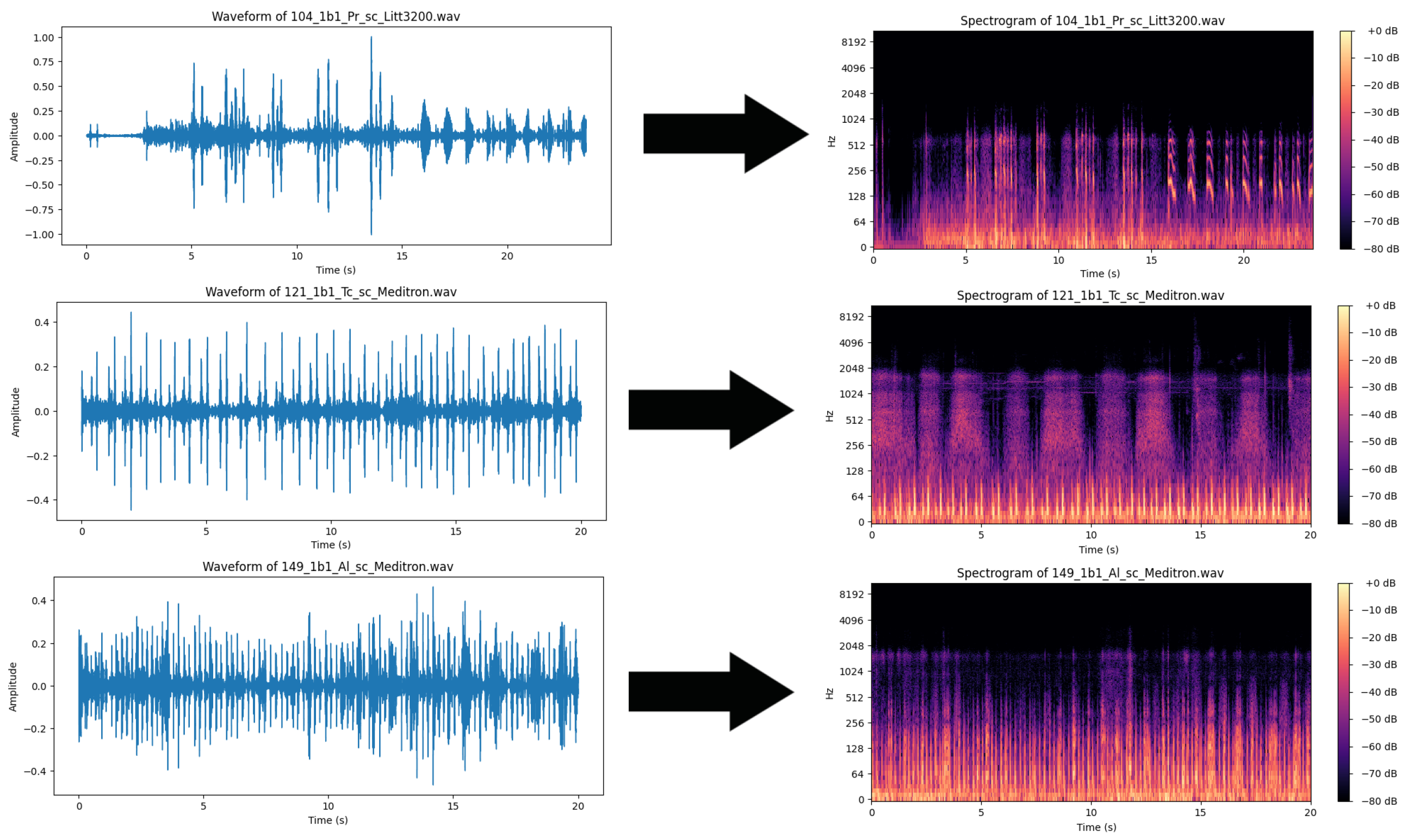
The format of the audio files makes them relatively poorly suitable for use with AI classifiers. While time-series classification may be applied, the intense computational demands of such an approach make it relatively inefficient. Furthermore, the large size of the dataset exacerbates these computational demands. Finally, much of the data in the audio file can be considered redundant. While manual filtering might be used to reduce and focus on certain frequencies, the use of mel spectrograms allows the audio file to be simultaneously observed across a spectrum. Additionally, mel spectrograms can be treated as images, making them well-suited for use with CNNs. The use of CNNs allows certain connections between neurons to be discarded as well as the use of filter kernels, thus reducing computational demands to some degree. In this work, the WAV audio files are converted into mel spectrogram images using the Librosa Python library. Images are then labeled according to the condition of the patient. Training is facilitated using 70% of the samples, while 30% are reserved for testing the trained models. A sample of generated spectrograms can be observed in Figure 1.

Figure 1.
Audio samples of healthy patient and patients with bronchitis and chronic obstructive pulmonary disease conversion to mel spectrograms.
Once inputs are established, the next step is to determine suitable network architectures and appropriate training parameters for the networks. Due to the large search spaces for potential solutions, traditional methods such as grid search would be ineffective. Therefore, metaheuristic optimizers are employed to optimize both network architecture and training parameters. The parameters and their experimental ranges are empirically determined to have the highest impact on performance. These include the number of CNN layers and fully connected layers in the networks as well as the number of neurons in each individual layer. Additionally, the number of training epochs is tuned alongside the learning rate and dropout probability. The respective parameter ranges are provided in Table 1.

Table 1.
Hyperparameters and their respective ranges.
Given the computational intensity of training deep learning models, the experimental setup is constrained to a maximum of eight iterations () per run, with each run utilizing only six solution candidates. We use 30 runs for each experiment to account for the stochastic nature of the metaheuristic optimization processes. These settings make the experiments computationally feasible and assure the repeatability of the results.
To meet the demands of this study, a modified version of the recently introduced EHO, called AGbAEHO, is utilized. The algorithm is utilized to optimize the CNN through an iterative process of hyperparameter tuning. To assess the performance of the introduced approach, it is compared to the original EHO [21]. Additionally, several state-of-the-art optimizers are also included in a comparative analysis. All algorithms are independently implemented for this study in Python. Each optimizer is issued six agents, with eight iterations allocated to improve outcomes. Algorithms chosen for the comparative analysis include the GA [96], PSO [66], the ABC [97], the FA [69], SCHO [98] and the COLSHADE [74] algorithm. Optimizers are implemented with the default parameter suggested in the respective source works that introduced each algorithm.
As the evaluated algorithms optimized classification models, several metrics are included in the assessment to ensure a thorough evaluation. Apart from the standard accuracy, precision, recall and f1-score metrics shown in Equations (16)–(19), the Cohen’s kappa [99] statistic is also tracked during experimentation and calculated according to Equation (20).
where , , and denote true positive, true negative, false positive and false negative values, respectively.
where represents an observed value while is the expected. Cohen’s kappa is well suited for working with imbalanced data, such as the dataset utilized in this work, and it is therefore utilized as an objective function. Alongside the objective function, the indicator function is tracked. In the case of this work, the indicator function is the error rate determined as . This metric is a fairly intuitive way of understanding the outcomes. Two sets of experiments are conducted: the first explores the detection of respiratory condition detection, and the second evaluates the potential of identifying specific types of conditions.
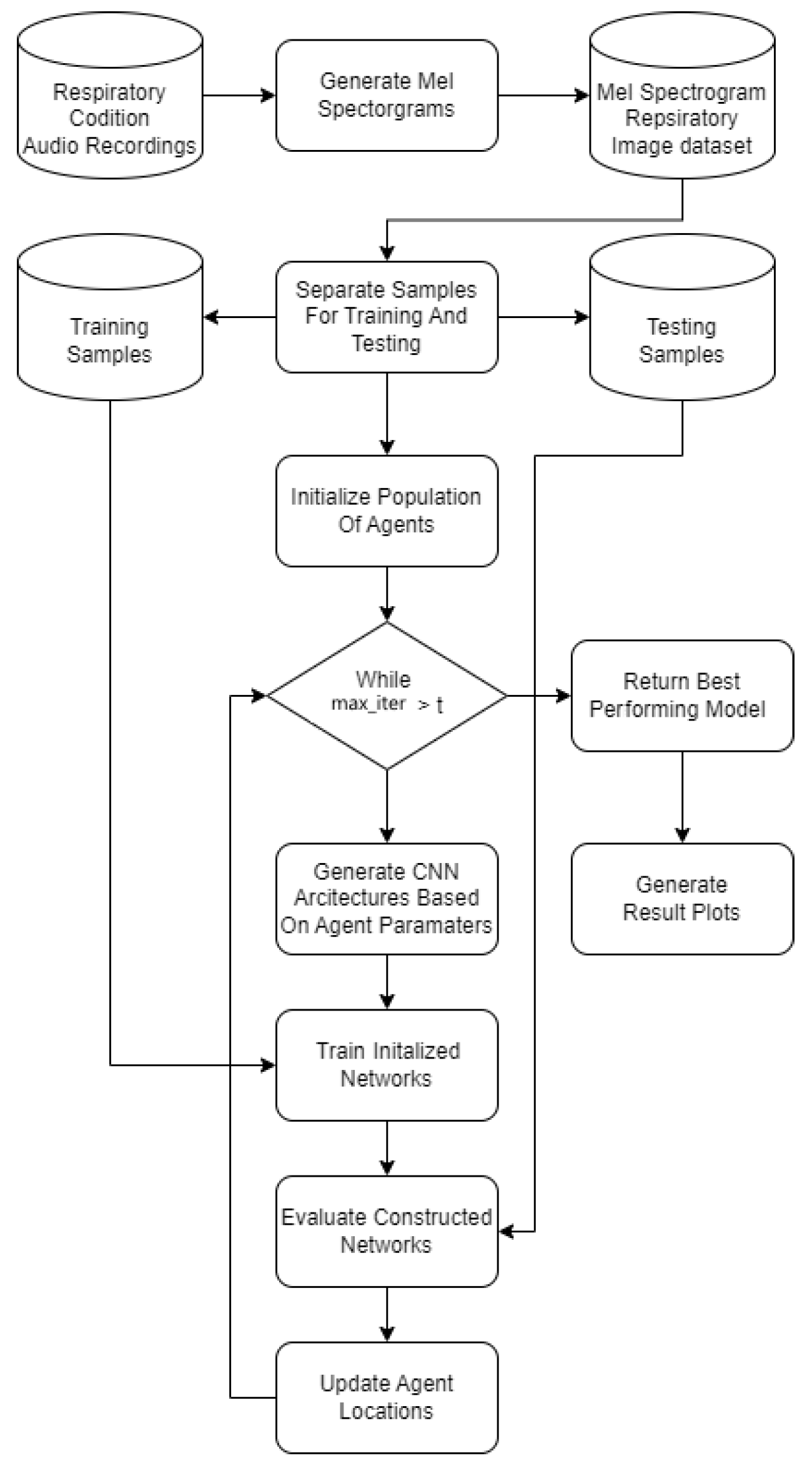
A flowchart of the introduced framework is presented in Figure 2.

Figure 2.
Introduced experimental framework flowchart.
5. Results
Two experimental evaluations are conducted in this work. The first experiment tackled the binary classification between healthy individuals and individuals affected by a respiratory condition. The second experiment tweaked classifiers with a multiclass classification in order to detect the specific condition in question.
5.1. Respiratory Condition Detection Simulations
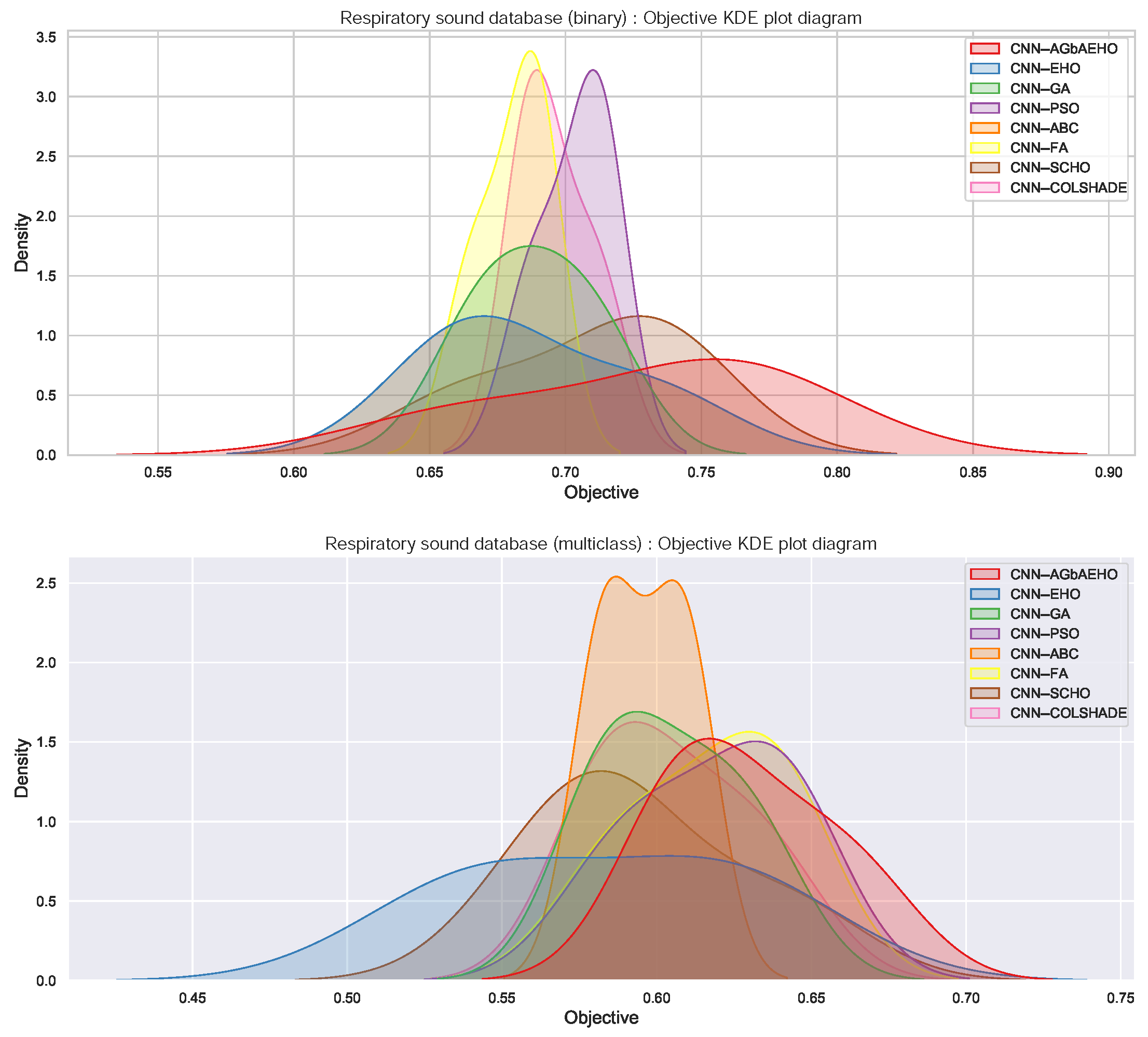
Respiratory condition detection outcomes in terms of objective function are provided in Table 2, which is followed by indicator function outcomes provided in Table 3. In both cases, the best-performing algorithm is the introduced modified metaheuristic. The best-performing algorithm demonstrated a Cohen’s kappa score of 0.76 in the best case. Scores of 0.729 and 0.76 were attained in the best and worst execution cases. Additionally, the FA showcases admirable stability when considering the objective function, despite not demonstrating the best outcomes. Kernel density estimation (KDE) plots were utilized to illustrate the distribution of Cohen’s kappa scores over 30 runs. The top plot in Figure 3 corresponds to the binary classification task and captures the stability of each method. Due to near-identical outcomes across the multiple independent runs for the top methods, minimal variance is observed that would not significantly influence the results of a Wilcoxon rank-sum test; hence, it is set aside.

Table 2.
Binary respiratory condition detection objective function outcomes. Best results are written in bold.

Table 3.
Binary respiratory condition detection indicator function outcomes. Best results are written in bold.

Figure 3.
KDE plot illustrating the comparison between the distribution of the results for the used methods for the binary (top) and multiclass (bottom) classifications.
In terms of indicator function outcomes, the introduced modified algorithm showcases similar outcomes with the best results shown in the best-case execution, with an error rate of 0.067. The introduced algorithm also attains the best results in the mean and medial cases, attaining error rates of 0.078 and 0.067, respectively.
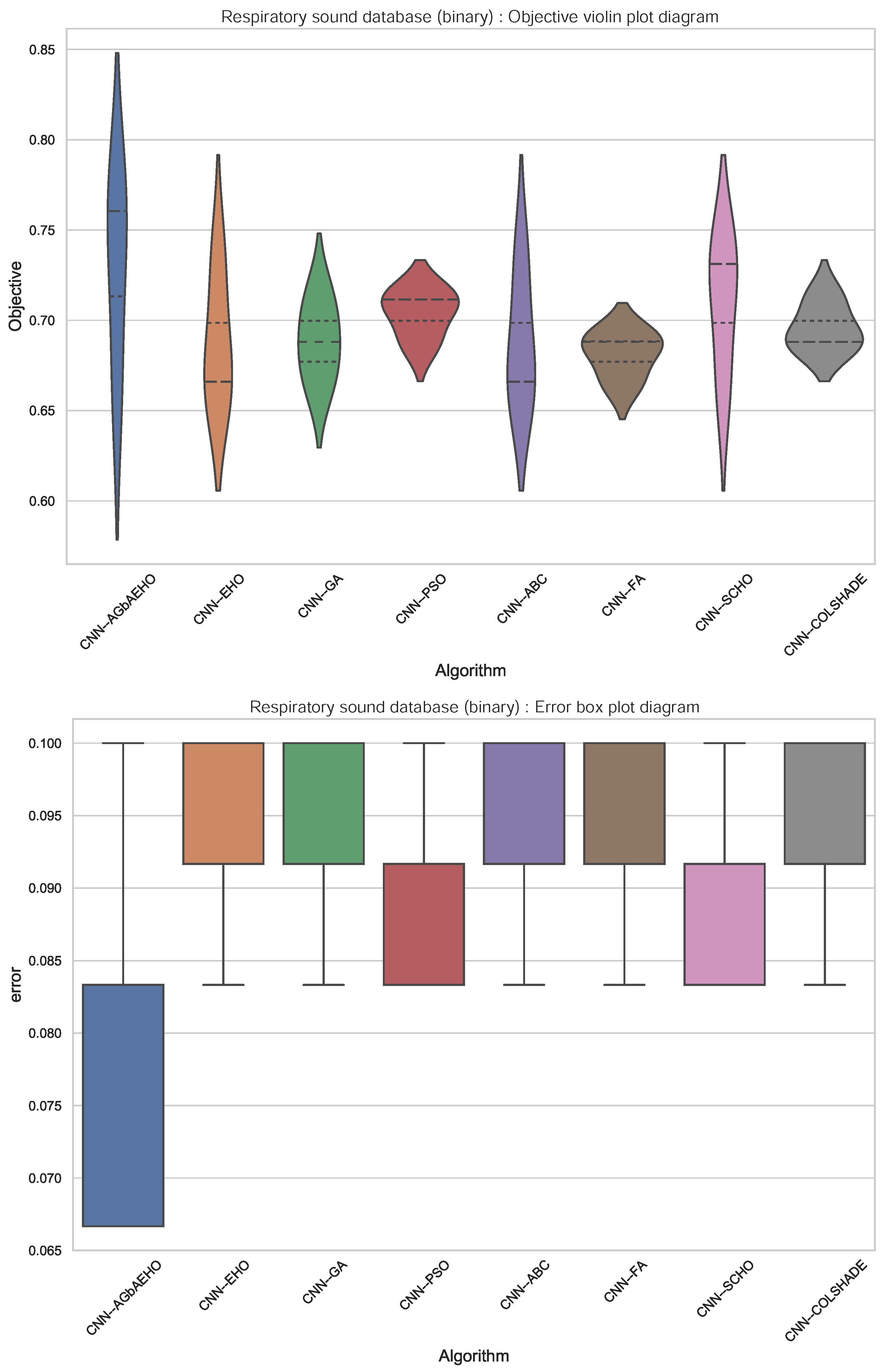
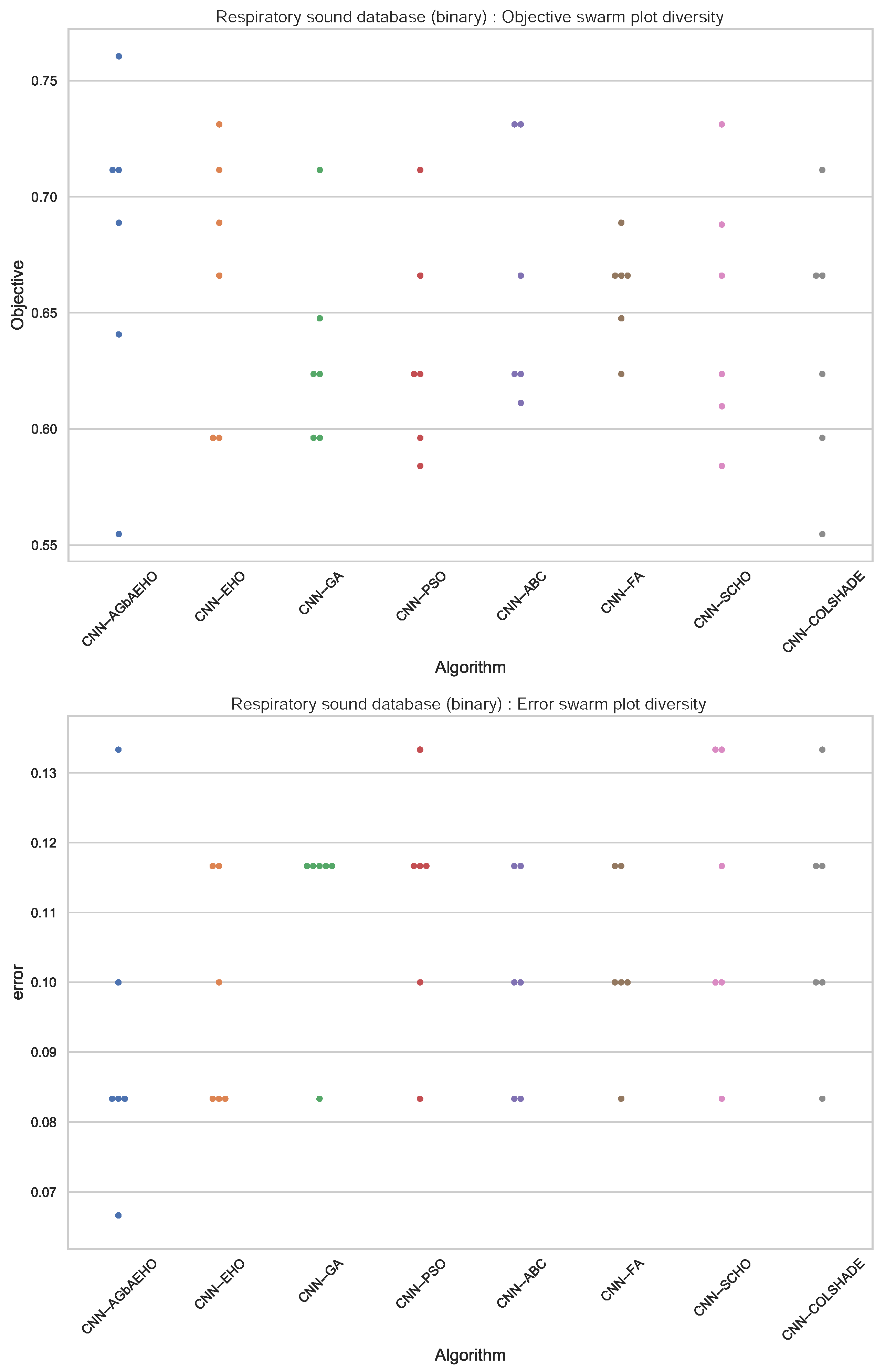
Further comparisons in terms of algorithm stability are provided in Figure 4. While the introduced algorithm sacrifices some stability for better outcomes, a strong grouping of solutions around the best outcome can be observed. This is further reinforced in the swarm plots provided in Figure 5.

Figure 4.
Binary respiratory condition detection outcome distribution plots.
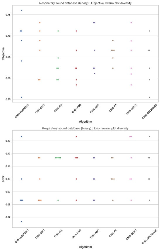
Figure 5.
Binary respiratory condition detection swarm plots.
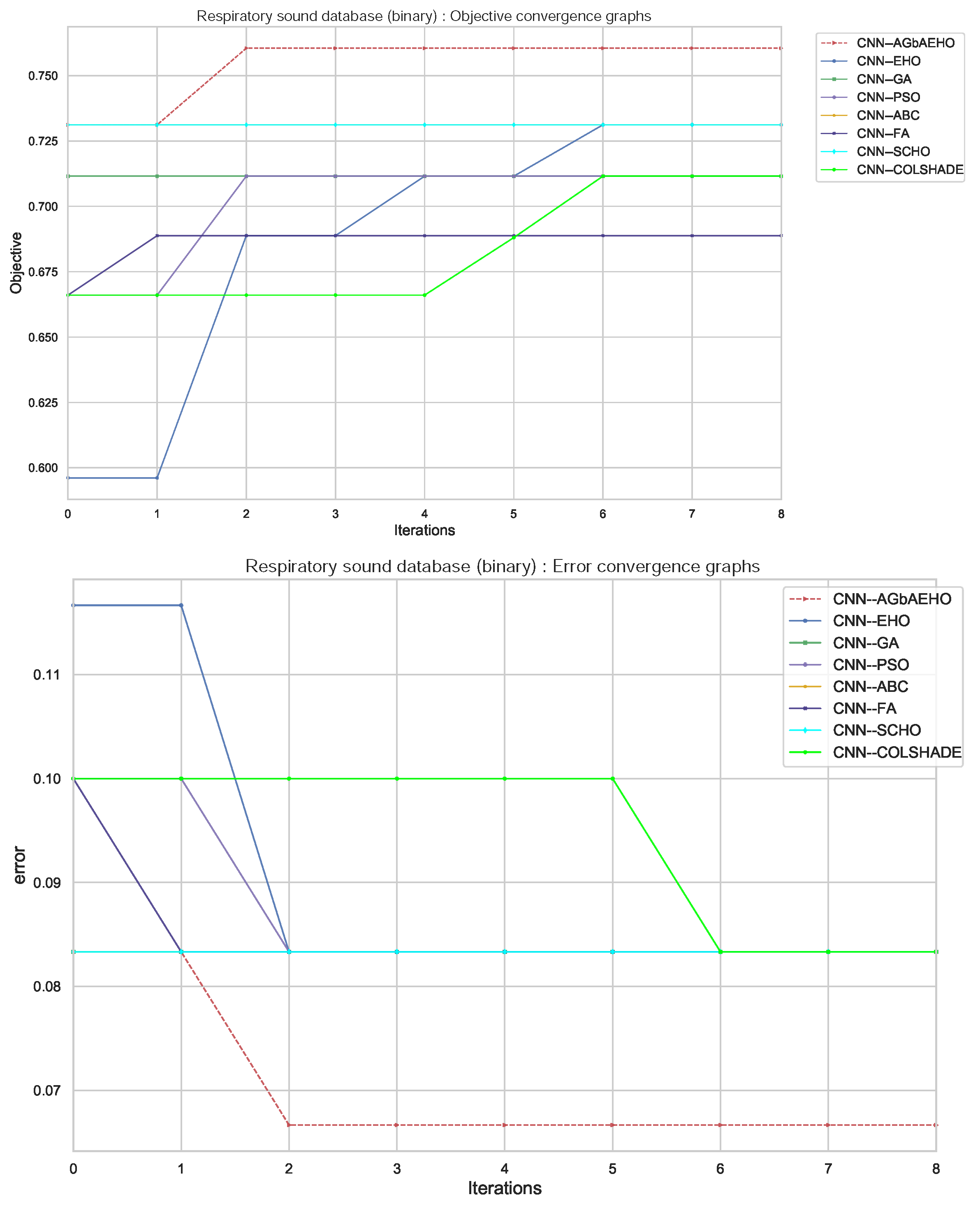
Additional information on the behaviors of each algorithm can be observed in Figure 6. Conversion rates for both the indicator and objective functions suggest that the boost in exploration, attained through the introduction of the modified mechanisms into the original algorithm, boosts the ability of the optimizer to avoid local optima and converge towards a better solution quickly.

Figure 6.
Binary respiratory condition detection convergence diagrams.
Detail metrics for each best-performing model optimized by each algorithm are provided in Table 4. A clear advantage can be observed in the models optimized by the introduced algorithm, demonstrating the highest procession scores for healthy patient detection as well as an accuracy of 0.933 and the highest macro and weighted averages for precision and f1-score.

Table 4.
Binary respiratory condition detection detail metrics for each model. Best results are written in bold.
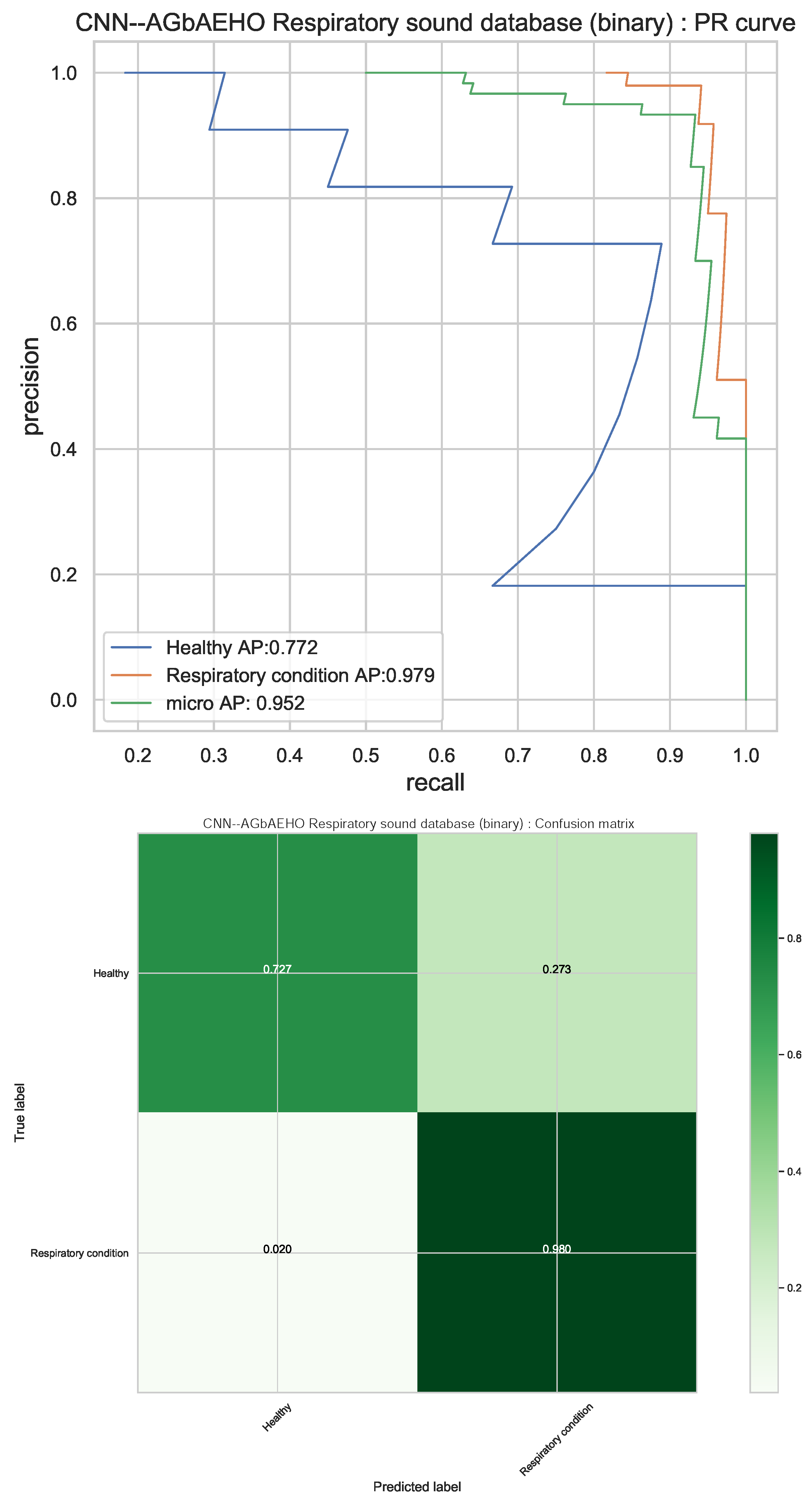
Additional details for the best-performing model optimized by the introduced algorithm can be visually considered in Figure 7 in the confusion matrix and PR curves. The models demonstrate a high rate of condition detection, with only a small fraction of healthy patients being misclassified as sick.

Figure 7.
Best-performing classifiers (CNN–AGbAEHO) model PR and confusion matrix charts.
Finally, to establish experimental repeatability, parameter selections for the best-performing models optimized by each algorithm are provided in Table 5.

Table 5.
Binary respiratory conduction detection parameter selections for each model. We denote by “lr”, “drop” and “Dense-L” the learning rate, dropout and the number of dense layers, respectively. Only one CNN layer is used in all cases. DL2 does not have a value when there is only one dense layer.
5.2. Respiratory Condition Identification Simulations
Respiratory condition identification outcomes in terms of objective function are provided in Table 6, followed by indicator function outcomes provided in Table 7. In both cases, the best-performing algorithm is the introduced modified metaheuristic. The best-performing algorithm demonstrated a Cohen’s kappa score of 0.666 in the best case. Scores of 0.63 and 0.623 were attained in the best and worst execution cases. When tackling multiclass classifications, the ABC algorithm showcases the highest rate of stability. KDE plots from the bottom plot in Figure 3 illustrate the distribution of Cohen’s kappa scores over 30 runs for the multiclass case.

Table 6.
Respiratory conduction identification objective function outcomes. Best results are written in bold.

Table 7.
Respiratory conduction identification indicator function outcomes. Best results are written in bold.
In terms of indicator function outcomes, the introduced modified algorithm showcases similar outcomes, with the best results shown in the best-case execution with an error rate of 0.25, which is the best score compared to other optimizers. Additionally, the best outcomes in terms of worst and mean outcomes are attained, matching the best performance in the median outcomes. Additionally, the stability is matched with other best-performing models.
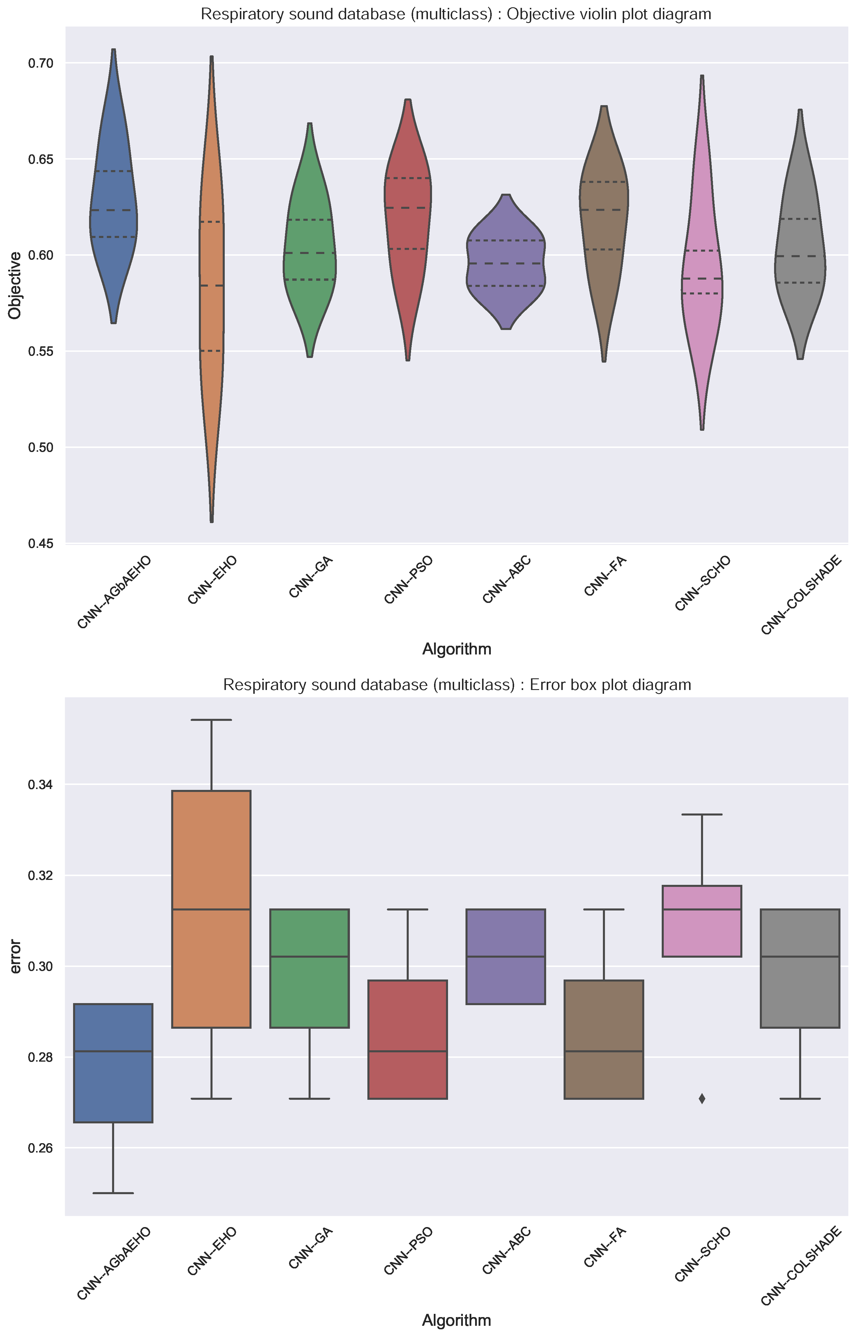
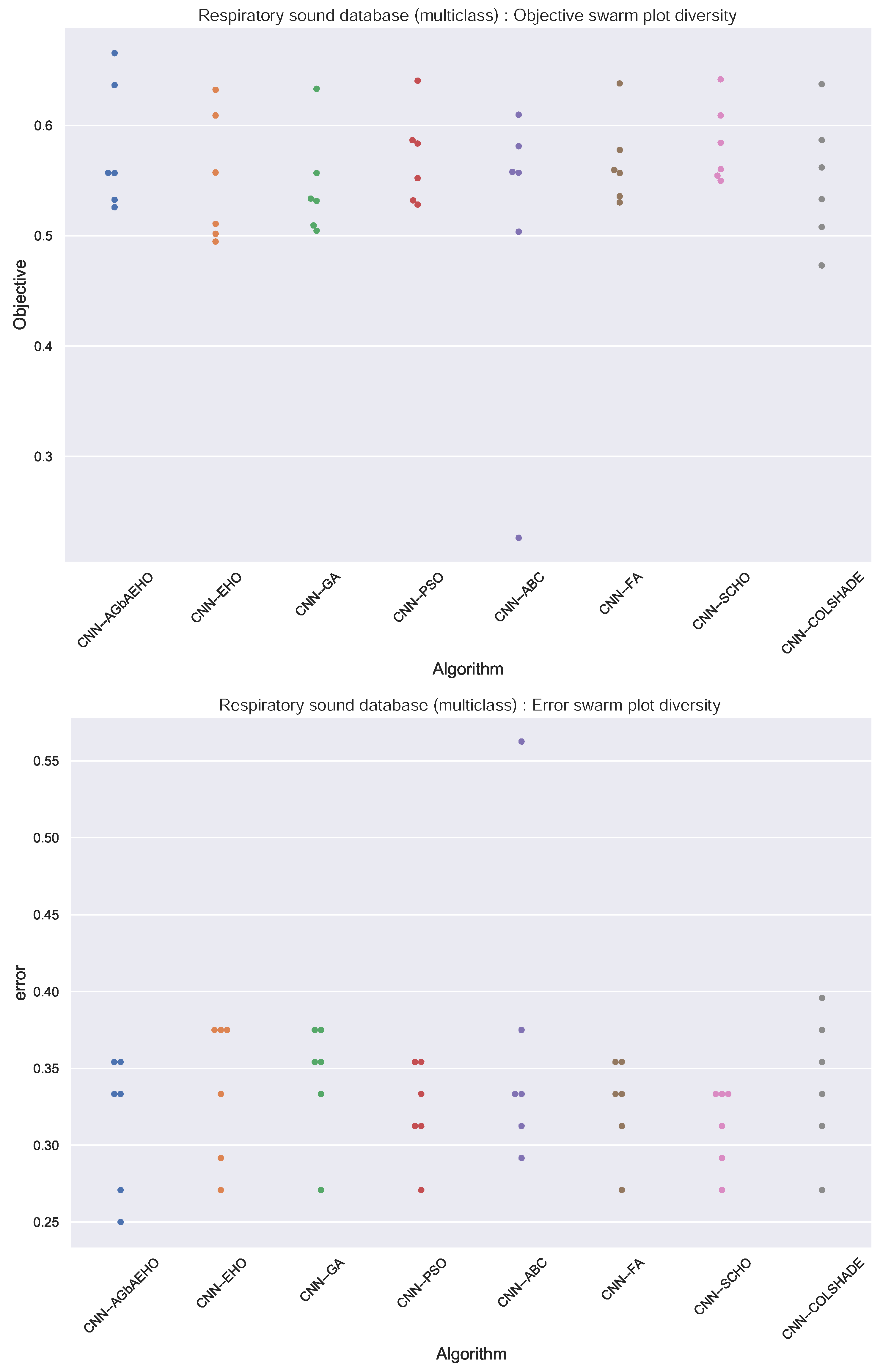
Further comparisons in terms of algorithm stability are provided in Figure 8. In the case of multiclass classification, the stability of the introduced algorithm is improved in comparison to the base optimizer, and better outcomes are attained overall in comparison to the base and other optimizers. This is further reinforced in the swarm plots provided in Figure 9.

Figure 8.
Respiratory conduction identification outcome distribution plots.

Figure 9.
Respiratory conduction identification swarm plots.
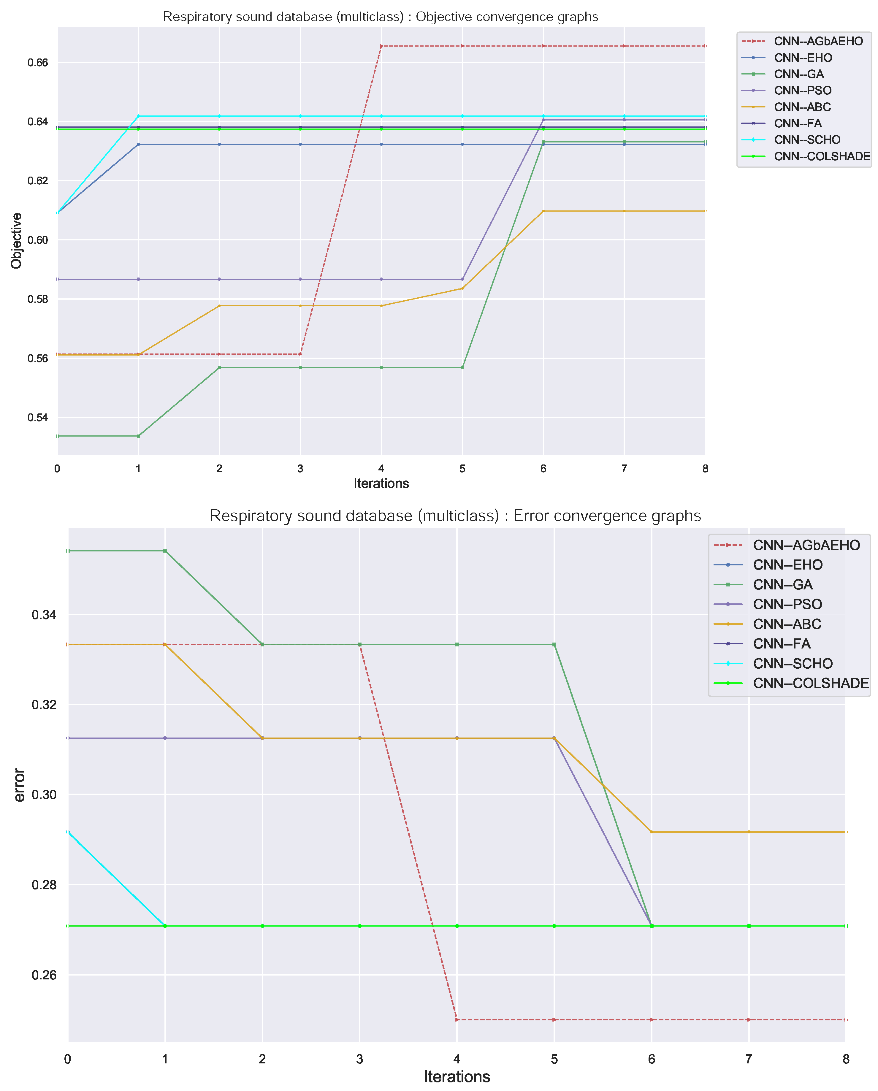
Algorithm convergence rates provide insight into the balance between the exploration and exploitation of optimizers. The convergence rates of respiratory condition identification from models constructed by each optimizer are provided in Figure 10. An overall improvement can be observed in the ability of the introduced algorithm to locate an optimal solution, with the algorithm avoiding local optima and finding a more promising solution within the search space.

Figure 10.
Respiratory conduction identification convergence diagrams.
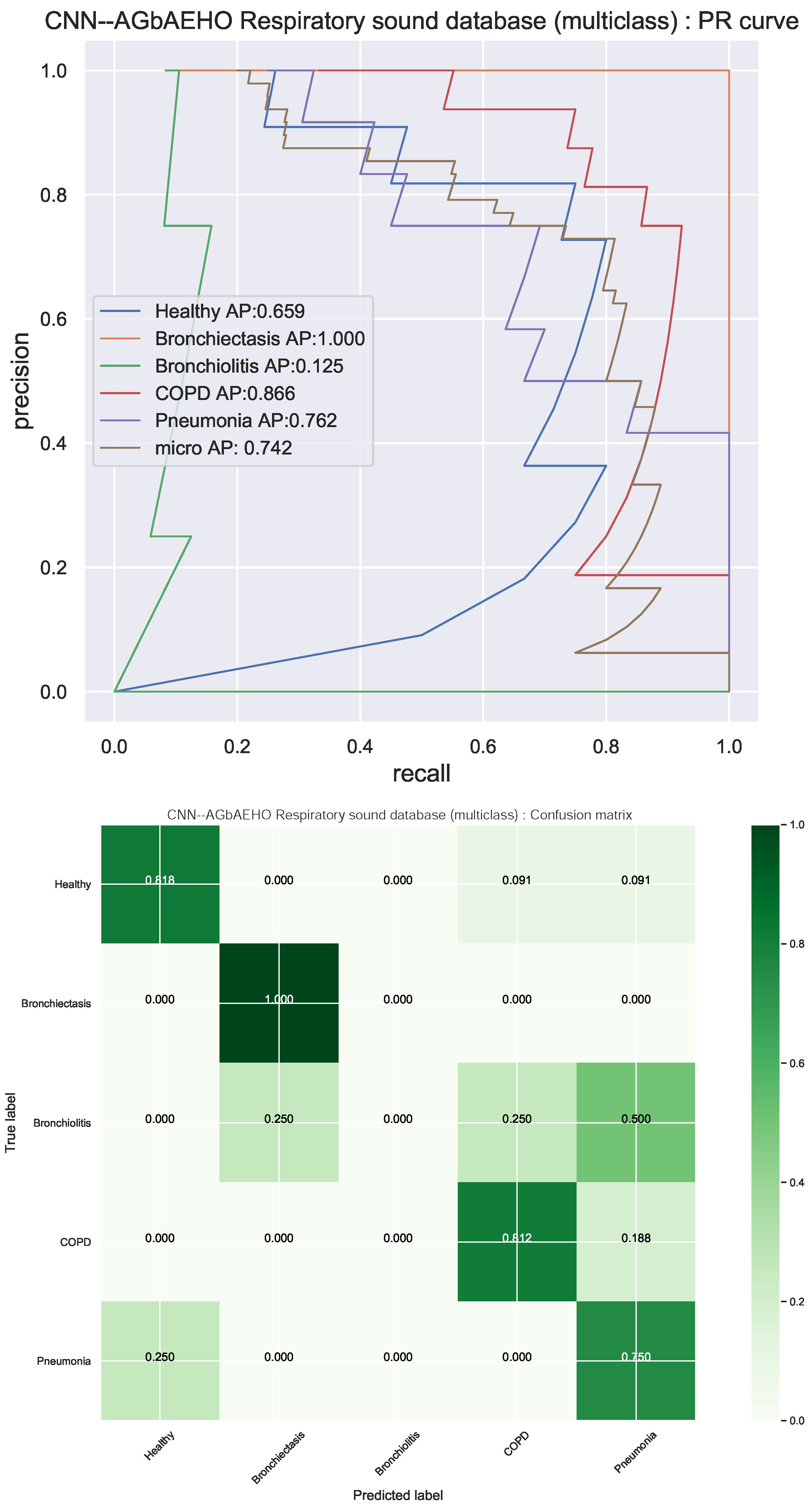
Detail metrics for each best-performing model optimized by each algorithm are provided in Table 8 and Table 9. An important note to be made is that all models struggle with bronchiectasis detection, leading to many misclassifications. It is also important to note that when handling medical diagnoses, especially the detection of specific conditions, many factors are combined alongside breading sounds. This limits the algorithm’s information input and, therefore, its ability for accurate identification. Decent precision can be observed for healthy individuals. Furthermore, an accuracy of 0.75 is attained by the best-performing models that are optimized by the introduced algorithm.

Table 8.
Respiratory conduction identification detail metrics for each class separately and for each model. We denote by “bronchiec”, “bronchio” and “pneum” the bronchiectasis, bronchiolitis and pneumonia classes, respectively. Best results are written in bold.

Table 9.
Respiratory conduction identification detail metrics for each model. Best results are written in bold.
The PR curves and confusion matrix for the best model are provided in Figure 11. The constructed models struggle with bronchiectasis detection and often misclassify conditions such as pneumonia or COPD. However, healthy individuals are well identified and are rarely confused with individuals with pneumonia. The parameter selection for each model is provided in Table 10 and Table 11 to facilitate experimental repeatability.

Figure 11.
Respiratory conduction identification best-performing classifiers (CNN–AGbAEHO) model PR and confusion matrix charts.

Table 10.
Selection for a subset of parameters for respiratory conduction identification for each model.

Table 11.
Selection for parameters related to layers for respiratory conduction identification for each model.
6. Conclusions
This work examines the diagnostic potential of AI for respiratory illness detection, emphasizing the value of prompt diagnosis and treatment in enhancing patient outcomes in a range of healthcare environments. By using audio analysis and CNNs, a potentially helpful way to determine patients’ respiratory problems is introduced. Due to the heavy dependence of classifiers on algorithm performance, a modified version of a metaheuristic optimizer is introduced. Simulations using mel spectrograms of patients’ breathing patterns, in particular, demonstrate the potential of this method in respiratory condition detection and multiclass classification scenarios. An accuracy of 0.933 is demonstrated for condition detection, with specific condition classification demonstrating an accuracy of 0.75.
Notwithstanding these encouraging results, it is critical to recognize the inherent limits of this work. The limited data availability makes it difficult to investigate a wider range of respiratory diseases, and the computing requirements of optimization limit the thorough investigation of different optimizers. Future works hope to further refine the proposed methodology and address some of the observed limitations as additional computational resources and data become available.
Author Contributions
Methodology, N.B., M.Z. and C.S.; Conceptualization, R.S., M.A. and M.D.; Writing—original draft, L.J. and M.Z.; Writing—review and editing, M.D. and M.A.; Visualization, N.B. and L.J.; Funding acquisition, C.S. and R.S.; Project administration, N.B. and L.J.; Supervision, M.D. and M.A. All authors have read and agreed to the published version of the manuscript.
Funding
This research was supported by the Science Fund of the Republic of Serbia, grant No. 7373, characterizing crises-caused air pollution alternations using an artificial intelligence-based framework (crAIRsis), and grant No. 7502, Intelligent Multi-Agent Control and Optimization applied to Green Buildings and Environmental Monitoring Drone Swarms (ECOSwarm).
Institutional Review Board Statement
Not applicable.
Informed Consent Statement
Not applicable.
Data Availability Statement
The dataset used in this study is freely available at the following URL: https://www.kaggle.com/datasets/vbookshelf/respiratory-sound-database (accessed on 12 January 2024).
Conflicts of Interest
The authors declare no conflicts of interest.
Abbreviations
The following abbreviations are used in this manuscript:
| CNN | convolutional neural network |
| EHO | elk herd optimizer |
| AGbAEHO | accelerated guided best adaptive elk herd optimizer |
| GA | genetic algorithm |
| PSO | particle swarm optimization |
| ABC | artificial bee colony |
| SCHO | sinsh cosh optimizer |
| FA | firefly algorithm |
References
- Labaki, W.W.; Han, M.K. Chronic respiratory diseases: A global view. Lancet Respir. Med. 2020, 8, 531–533. [Google Scholar] [CrossRef] [PubMed]
- Ciotti, M.; Ciccozzi, M.; Terrinoni, A.; Jiang, W.C.; Wang, C.B.; Bernardini, S. The COVID-19 pandemic. Crit. Rev. Clin. Lab. Sci. 2020, 57, 365–388. [Google Scholar] [CrossRef] [PubMed]
- Lindskou, T.A.; Pilgaard, L.; Søvsø, M.B.; Kløjgård, T.A.; Larsen, T.M.; Jensen, F.B.; Weinrich, U.M.; Christensen, E.F. Symptom, diagnosis and mortality among respiratory emergency medical service patients. PLoS ONE 2019, 14, e0213145. [Google Scholar] [CrossRef] [PubMed]
- Levy, M.L.; Fletcher, M.; Price, D.B.; Hausend, T.; Halbert, R.J.; Yawn, B.P. International Primary Care Respiratory Group (IPCRG) Guidelines: Diagnosis of respiratory diseases in primary care. Prim. Care Respir. J. 2006, 15, 20–34. [Google Scholar] [CrossRef] [PubMed]
- Chang, L.H.; Rivera, M.P. Respiratory diseases: Meeting the challenges of screening, prevention, and treatment. N. Carol. Med. J. 2013, 74, 385–392. [Google Scholar] [CrossRef]
- Arvind, S.; Tembhurne, J.V.; Diwan, T.; Sahare, P. Improvised light weight deep CNN based U-Net for the semantic segmentation of lungs from chest X-rays. Results Eng. 2023, 17, 100929. [Google Scholar] [CrossRef]
- Rao, G.E.; Rajitha, B.; Srinivasu, P.N.; Ijaz, M.F.; Woźniak, M. Hybrid framework for respiratory lung diseases detection based on classical CNN and quantum classifiers from chest X-rays. Biomed. Signal Process. Control 2024, 88, 105567. [Google Scholar] [CrossRef]
- Wall, C.; Zhang, L.; Yu, Y.; Mistry, K. Deep recurrent neural networks with attention mechanisms for respiratory anomaly classification. In Proceedings of the 2021 International Joint Conference on Neural Networks (IJCNN), Shenzhen, China, 18–22 July 2021; pp. 1–8. [Google Scholar]
- Mosier, J.M.; Nayebi, A.; Fisher, J.M.; Subbian, V. Predicting Failure of Noninvasive Respiratory Support Using Deep Recurrent Learning. Respir. Care 2023, 68, 488–496. [Google Scholar]
- Mekov, E.; Miravitlles, M.; Petkov, R. Artificial intelligence and machine learning in respiratory medicine. Expert Rev. Respir. Med. 2020, 14, 559–564. [Google Scholar] [CrossRef]
- Ferrari, D.; Milic, J.; Tonelli, R.; Ghinelli, F.; Meschiari, M.; Volpi, S.; Faltoni, M.; Franceschi, G.; Iadisernia, V.; Yaacoub, D.; et al. Machine learning in predicting respiratory failure in patients with COVID-19 pneumonia—Challenges, strengths, and opportunities in a global health emergency. PLoS ONE 2020, 15, e0239172. [Google Scholar] [CrossRef]
- Patel, D.; Kher, V.; Desai, B.; Lei, X.; Cen, S.; Nanda, N.; Gholamrezanezhad, A.; Duddalwar, V.; Varghese, B.; Oberai, A.A. Machine learning based predictors for COVID-19 disease severity. Sci. Rep. 2021, 11, 4673. [Google Scholar] [CrossRef] [PubMed]
- Ramudu, K.; Mohan, V.M.; Jyothirmai, D.; Prasad, D.; Agrawal, R.; Boopathi, S. Machine learning and artificial intelligence in disease prediction: Applications, challenges, limitations, case studies, and future directions. In Contemporary Applications of Data Fusion for Advanced Healthcare Informatics; IGI Global: Hershey, PA, USA, 2023; pp. 297–318. [Google Scholar]
- Mittermaier, M.; Raza, M.M.; Kvedar, J.C. Bias in AI-based models for medical applications: Challenges and mitigation strategies. NPJ Digit. Med. 2023, 6, 113. [Google Scholar] [CrossRef] [PubMed]
- Chaddad, A.; Peng, J.; Xu, J.; Bouridane, A. Survey of explainable AI techniques in healthcare. Sensors 2023, 23, 634. [Google Scholar] [CrossRef] [PubMed]
- Wolpert, D.H.; Macready, W.G. No free lunch theorems for optimization. IEEE Trans. Evol. Comput. 1997, 1, 67–82. [Google Scholar] [CrossRef]
- Eiben, A.E.; Smit, S.K. Evolutionary Algorithm Parameters and Methods to Tune Them. In Autonomous Search; Hamadi, Y., Monfroy, E., Saubion, F., Eds.; Springer: Berlin/Heidelberg, Germany, 2012; pp. 15–36. [Google Scholar] [CrossRef]
- Tatsis, V.A.; Parsopoulos, K.E. Reinforcement learning for enhanced online gradient-based parameter adaptation in metaheuristics. Swarm Evol. Comput. 2023, 83, 101371. [Google Scholar] [CrossRef]
- Bartz-Beielstein, T.; Preuss, M. Experimental research in evolutionary computation. In Proceedings of the 9th Annual Conference Companion on Genetic and Evolutionary Computation, London, UK, 7–11 July 2007; pp. 3001–3020. [Google Scholar] [CrossRef]
- Birattari, M.; Yuan, Z.; Balaprakash, P.; Stützle, T. F-Race and Iterated F-Race: An Overview. In Experimental Methods for the Analysis of Optimization Algorithms; Bartz-Beielstein, T., Chiarandini, M., Paquete, L., Preuss, M., Eds.; Springer: Berlin/Heidelberg, Germany, 2010; pp. 311–336. [Google Scholar] [CrossRef]
- Al-Betar, M.A.; Awadallah, M.A.; Braik, M.S.; Makhadmeh, S.; Doush, I.A. Elk herd optimizer: A novel nature-inspired metaheuristic algorithm. Artif. Intell. Rev. 2024, 57, 48. [Google Scholar] [CrossRef]
- Haick, H.; Tang, N. Artificial intelligence in medical sensors for clinical decisions. ACS Nano 2021, 15, 3557–3567. [Google Scholar] [CrossRef] [PubMed]
- Fujita, H. AI-based computer-aided diagnosis (AI-CAD): The latest review to read first. Radiol. Phys. Technol. 2020, 13, 6–19. [Google Scholar] [CrossRef] [PubMed]
- Ahmad, Z.; Rahim, S.; Zubair, M.; Abdul-Ghafar, J. Artificial intelligence (AI) in medicine, current applications and future role with special emphasis on its potential and promise in pathology: Present and future impact, obstacles including costs and acceptance among pathologists, practical and philosophical considerations. A comprehensive review. Diagn. Pathol. 2021, 16, 24. [Google Scholar]
- Bezdan, T.; Zivkovic, M.; Tuba, E.; Strumberger, I.; Bacanin, N.; Tuba, M. Glioma brain tumor grade classification from mri using convolutional neural networks designed by modified fa. In Proceedings of the International Conference on Intelligent and Fuzzy Systems, Turkey, Izmir, 21–23 July 2020; Springer: Berlin/Heidelberg, Germany, 2020; pp. 955–963. [Google Scholar]
- Tiwari, P.; Pant, B.; Elarabawy, M.M.; Abd-Elnaby, M.; Mohd, N.; Dhiman, G.; Sharma, S. Cnn based multiclass brain tumor detection using medical imaging. Comput. Intell. Neurosci. 2022, 2022, 1830010. [Google Scholar] [CrossRef]
- Sarvamangala, D.; Kulkarni, R.V. Convolutional neural networks in medical image understanding: A survey. Evol. Intell. 2022, 15, 1–22. [Google Scholar] [CrossRef] [PubMed]
- Cuk, A.; Bezdan, T.; Jovanovic, L.; Antonijevic, M.; Stankovic, M.; Simic, V.; Zivkovic, M.; Bacanin, N. Tuning attention based long-short term memory neural networks for Parkinson’s disease detection using modified metaheuristics. Sci. Rep. 2024, 14, 4309. [Google Scholar] [CrossRef] [PubMed]
- Fujita, T.; Luo, Z.; Quan, C.; Mori, K.; Cao, S. Performance evaluation of RNN with hyperbolic secant in gate structure through application of Parkinson’s disease detection. Appl. Sci. 2021, 11, 4361. [Google Scholar] [CrossRef]
- Minic, A.; Jovanovic, L.; Bacanin, N.; Stoean, C.; Zivkovic, M.; Spalevic, P.; Petrovic, A.; Dobrojevic, M.; Stoean, R. Applying Recurrent Neural Networks for Anomaly Detection in Electrocardiogram Sensor Data. Sensors 2023, 23, 9878. [Google Scholar] [CrossRef] [PubMed]
- Kuila, S.; Dhanda, N.; Joardar, S. ECG signal classification and arrhythmia detection using ELM-RNN. Multimed. Tools Appl. 2022, 81, 25233–25249. [Google Scholar] [CrossRef]
- Kim, B.H.; Pyun, J.Y. ECG identification for personal authentication using LSTM-based deep recurrent neural networks. Sensors 2020, 20, 3069. [Google Scholar] [CrossRef] [PubMed]
- Pilcevic, D.; Djuric Jovicic, M.; Antonijevic, M.; Bacanin, N.; Zivkovic, M. Performance evaluation of metaheuristics-tuned recurrent neural networks for electroencephalography anomaly detection. Front. Physiol. 2023, 14, 1267011. [Google Scholar] [CrossRef] [PubMed]
- Supakar, R.; Satvaya, P.; Chakrabarti, P. A deep learning based model using RNN-LSTM for the Detection of Schizophrenia from EEG data. Comput. Biol. Med. 2022, 151, 106225. [Google Scholar] [CrossRef]
- Bouallegue, G.; Djemal, R.; Alshebeili, S.A.; Aldhalaan, H. A dynamic filtering DF-RNN deep-learning-based approach for EEG-based neurological disorders diagnosis. IEEE Access 2020, 8, 206992–207007. [Google Scholar] [CrossRef]
- Kaplan, A.; Cao, H.; FitzGerald, J.M.; Iannotti, N.; Yang, E.; Kocks, J.W.; Kostikas, K.; Price, D.; Reddel, H.K.; Tsiligianni, I.; et al. Artificial intelligence/machine learning in respiratory medicine and potential role in asthma and COPD diagnosis. J. Allergy Clin. Immunol. Pract. 2021, 9, 2255–2261. [Google Scholar] [CrossRef]
- Chen, K.C.; Yu, H.R.; Chen, W.S.; Lin, W.C.; Lee, Y.C.; Chen, H.H.; Jiang, J.H.; Su, T.Y.; Tsai, C.K.; Tsai, T.A.; et al. Diagnosis of common pulmonary diseases in children by X-ray images and deep learning. Sci. Rep. 2020, 10, 17374. [Google Scholar] [CrossRef] [PubMed]
- Cao, X.F.; Li, Y.; Xin, H.N.; Zhang, H.R.; Pai, M.; Gao, L. Application of artificial intelligence in digital chest radiography reading for pulmonary tuberculosis screening. Chronic Dis. Transl. Med. 2021, 7, 35–40. [Google Scholar] [CrossRef] [PubMed]
- Qin, Z.Z.; Ahmed, S.; Sarker, M.S.; Paul, K.; Adel, A.S.S.; Naheyan, T.; Barrett, R.; Banu, S.; Creswell, J. Tuberculosis detection from chest X-rays for triaging in a high tuberculosis-burden setting: An evaluation of five artificial intelligence algorithms. Lancet Digit. Health 2021, 3, e543–e554. [Google Scholar] [CrossRef] [PubMed]
- Chamberlin, J.; Kocher, M.R.; Waltz, J.; Snoddy, M.; Stringer, N.F.; Stephenson, J.; Sahbaee, P.; Sharma, P.; Rapaka, S.; Schoepf, U.J.; et al. Automated detection of lung nodules and coronary artery calcium using artificial intelligence on low-dose CT scans for lung cancer screening: Accuracy and prognostic value. BMC Med. 2021, 19, 55. [Google Scholar] [CrossRef] [PubMed]
- Mei, X.; Lee, H.C.; Diao, K.y.; Huang, M.; Lin, B.; Liu, C.; Xie, Z.; Ma, Y.; Robson, P.M.; Chung, M.; et al. Artificial intelligence–enabled rapid diagnosis of patients with COVID-19. Nat. Med. 2020, 26, 1224–1228. [Google Scholar] [CrossRef]
- Ozsahin, I.; Sekeroglu, B.; Musa, M.S.; Mustapha, M.T.; Ozsahin, D.U. Review on diagnosis of COVID-19 from chest CT images using artificial intelligence. Comput. Math. Methods Med. 2020, 2020, 756518. [Google Scholar] [CrossRef]
- Almalki, Y.E.; Qayyum, A.; Irfan, M.; Haider, N.; Glowacz, A.; Alshehri, F.M.; Alduraibi, S.K.; Alshamrani, K.; Alkhalik Basha, M.A.; Alduraibi, A.; et al. A novel method for COVID-19 diagnosis using artificial intelligence in chest X-ray images. Healthcare 2021, 9, 522. [Google Scholar] [CrossRef]
- Laguarta, J.; Hueto, F.; Subirana, B. COVID-19 artificial intelligence diagnosis using only cough recordings. IEEE Open J. Eng. Med. Biol. 2020, 1, 275–281. [Google Scholar] [CrossRef]
- Santosh, K.; Rasmussen, N.; Mamun, M.; Aryal, S. A systematic review on cough sound analysis for COVID-19 diagnosis and screening: Is my cough sound COVID-19? PeerJ Comput. Sci. 2022, 8, e958. [Google Scholar] [CrossRef]
- Imran, A.; Posokhova, I.; Qureshi, H.N.; Masood, U.; Riaz, M.S.; Ali, K.; John, C.N.; Hussain, M.I.; Nabeel, M. AI4COVID-19: AI enabled preliminary diagnosis for COVID-19 from cough samples via an app. Inform. Med. Unlocked 2020, 20, 100378. [Google Scholar] [CrossRef]
- Ullah, W.; Hussain, T.; Ullah, F.U.M.; Lee, M.Y.; Baik, S.W. TransCNN: Hybrid CNN and transformer mechanism for surveillance anomaly detection. Eng. Appl. Artif. Intell. 2023, 123, 106173. [Google Scholar] [CrossRef]
- Liang, T.; Bao, H.; Pan, W.; Pan, F. Traffic sign detection via improved sparse R-CNN for autonomous vehicles. J. Adv. Transp. 2022, 2022, 3825532. [Google Scholar] [CrossRef]
- Tang, Y.; Chen, Y.; Sharifuzzaman, S.A.; Li, T. An automatic fine-grained violence detection system for animation based on modified faster R-CNN. Expert Syst. Appl. 2024, 237, 121691. [Google Scholar] [CrossRef]
- Song, P.; Li, P.; Dai, L.; Wang, T.; Chen, Z. Boosting R-CNN: Reweighting R-CNN samples by RPN’s error for underwater object detection. Neurocomputing 2023, 530, 150–164. [Google Scholar] [CrossRef]
- Yuan, F.; Zhang, Z.; Fang, Z. An effective CNN and Transformer complementary network for medical image segmentation. Pattern Recognit. 2023, 136, 109228. [Google Scholar] [CrossRef]
- Li, S.; Zhao, X. High-resolution concrete damage image synthesis using conditional generative adversarial network. Autom. Constr. 2023, 147, 104739. [Google Scholar] [CrossRef]
- Rajeshkumar, G.; Braveen, M.; Venkatesh, R.; Shermila, P.J.; Prabu, B.G.; Veerasamy, B.; Bharathi, B.; Jeyam, A. Smart office automation via faster R-CNN based face recognition and internet of things. Meas. Sens. 2023, 27, 100719. [Google Scholar] [CrossRef]
- He, L.; He, L.; Peng, L. CFormerFaceNet: Efficient lightweight network merging a CNN and transformer for face recognition. Appl. Sci. 2023, 13, 6506. [Google Scholar] [CrossRef]
- Kaluthantrige, A.; Feng, J.; Gil-Fernández, J. CNN-based Image Processing algorithm for autonomous optical navigation of Hera mission to the binary asteroid Didymos. Acta Astronaut. 2023, 211, 60–75. [Google Scholar] [CrossRef]
- Karim Amer, M.S.; Shaker, M.; ElHelw, M. Deep convolutional neural network based autonomous drone navigation. In Proceedings of the Thirteenth International Conference on Machine Vision, Rome, Italy, 2–6 November 2020; Volume 11605, p. 1160503. [Google Scholar]
- Alfred Daniel, J.; Chandru Vignesh, C.; Muthu, B.A.; Senthil Kumar, R.; Sivaparthipan, C.; Marin, C.E.M. Fully convolutional neural networks for LIDAR–camera fusion for pedestrian detection in autonomous vehicle. Multimed. Tools Appl. 2023, 82, 25107–25130. [Google Scholar] [CrossRef]
- Kaya, Ö.; Çodur, M.Y.; Mustafaraj, E. Automatic detection of pedestrian crosswalk with faster r-cnn and yolov7. Buildings 2023, 13, 1070. [Google Scholar] [CrossRef]
- Lilhore, U.K.; Simaiya, S.; Dalal, S.; Damaševičius, R. A smart waste classification model using hybrid CNN-LSTM with transfer learning for sustainable environment. In Multimedia Tools and Applications; Springer: Berlin/Heidelberg, Germany, 2023; pp. 1–25. [Google Scholar]
- Saponara, S.; Elhanashi, A.; Gagliardi, A. Real-time video fire/smoke detection based on CNN in antifire surveillance systems. J. Real-Time Image Process. 2021, 18, 889–900. [Google Scholar] [CrossRef]
- Kheddar, H.; Himeur, Y.; Al-Maadeed, S.; Amira, A.; Bensaali, F. Deep transfer learning for automatic speech recognition: Towards better generalization. Knowl.-Based Syst. 2023, 277, 110851. [Google Scholar] [CrossRef]
- Costantini, G.; Cesarini, V.; Di Leo, P.; Amato, F.; Suppa, A.; Asci, F.; Pisani, A.; Calculli, A.; Saggio, G. Artificial intelligence-based voice assessment of patients with Parkinson’s disease off and on treatment: Machine vs. deep-learning comparison. Sensors 2023, 23, 2293. [Google Scholar] [CrossRef] [PubMed]
- Foggia, P.; Petkov, N.; Saggese, A.; Strisciuglio, N.; Vento, M. Audio surveillance of roads: A system for detecting anomalous sounds. IEEE Trans. Intell. Transp. Syst. 2015, 17, 279–288. [Google Scholar] [CrossRef]
- Nourani, V.; Gökçekuş, H.; Umar, I.K. Artificial intelligence based ensemble model for prediction of vehicular traffic noise. Environ. Res. 2020, 180, 108852. [Google Scholar] [CrossRef] [PubMed]
- Singh, D.; Upadhyay, R.; Pannu, H.S.; Leray, D. Development of an adaptive neuro fuzzy inference system based vehicular traffic noise prediction model. J. Ambient Intell. Humaniz. Comput. 2021, 12, 2685–2701. [Google Scholar] [CrossRef]
- Eberhart, R.; Kennedy, J. Particle swarm optimization. In Proceedings of the IEEE International Conference on Neural Networks, Perth, WA, Australia, 27 November–1 December 1995; Citeseer: State College, PA, USA, 1995; Volume 4, pp. 1942–1948. [Google Scholar]
- Mirjalili, S.; Mirjalili, S. Genetic algorithm. In Evolutionary Algorithms and Neural Networks: Theory and Applications; Springer: Berlin/Heidelberg, Germany, 2019; pp. 43–55. [Google Scholar]
- Mirjalili, S. SCA: A sine cosine algorithm for solving optimization problems. Knowl.-Based Syst. 2016, 96, 120–133. [Google Scholar] [CrossRef]
- Yang, X.S.; Slowik, A. Firefly algorithm. In Swarm Intelligence Algorithms; CRC Press: Boca Raton, FL, USA, 2020; pp. 163–174. [Google Scholar]
- Faris, H.; Aljarah, I.; Al-Betar, M.A.; Mirjalili, S. Grey wolf optimizer: A review of recent variants and applications. Neural Comput. Appl. 2018, 30, 413–435. [Google Scholar] [CrossRef]
- Abualigah, L.; Abd Elaziz, M.; Sumari, P.; Geem, Z.W.; Gandomi, A.H. Reptile Search Algorithm (RSA): A nature-inspired meta-heuristic optimizer. Expert Syst. Appl. 2022, 191, 116158. [Google Scholar] [CrossRef]
- Połap, D.; Woźniak, M. Red fox optimization algorithm. Expert Syst. Appl. 2021, 166, 114107. [Google Scholar] [CrossRef]
- Polap, D.; Woźniak, M. Polar bear optimization algorithm: Meta-heuristic with fast population movement and dynamic birth and death mechanism. Symmetry 2017, 9, 203. [Google Scholar] [CrossRef]
- Gurrola-Ramos, J.; Hernàndez-Aguirre, A.; Dalmau-Cedeño, O. COLSHADE for real-world single-objective constrained optimization problems. In Proceedings of the 2020 IEEE congress on evolutionary computation (CEC), Glasgow, UK, 19–24 July 2020; pp. 1–8. [Google Scholar]
- Jovanovic, L.; Djuric, M.; Zivkovic, M.; Jovanovic, D.; Strumberger, I.; Antonijevic, M.; Budimirovic, N.; Bacanin, N. Tuning xgboost by planet optimization algorithm: An application for diabetes classification. In Proceedings of the Fourth International Conference on Communication, Computing and Electronics Systems: ICCCES 2022, Coimbatore, India, 15–16 September 2022; Springer: Berlin/Heidelberg, Germany, 2023; pp. 787–803. [Google Scholar]
- Petrovic, A.; Bacanin, N.; Zivkovic, M.; Marjanovic, M.; Antonijevic, M.; Strumberger, I. The adaboost approach tuned by firefly metaheuristics for fraud detection. In Proceedings of the 2022 IEEE World Conference on Applied Intelligence and Computing (AIC), Sonbhadra, India, 17–19 June 2022; pp. 834–839. [Google Scholar]
- Zamani, H.; Nadimi-Shahraki, M.H.; Gandomi, A.H. Starling murmuration optimizer: A novel bio-inspired algorithm for global and engineering optimization. Comput. Methods Appl. Mech. Eng. 2022, 392, 114616. [Google Scholar] [CrossRef]
- Nadimi-Shahraki, M.H.; Zamani, H. DMDE: Diversity-maintained multi-trial vector differential evolution algorithm for non-decomposition large-scale global optimization. Expert Syst. Appl. 2022, 198, 116895. [Google Scholar] [CrossRef]
- Predić, B.; Jovanovic, L.; Simic, V.; Bacanin, N.; Zivkovic, M.; Spalevic, P.; Budimirovic, N.; Dobrojevic, M. Cloud-load forecasting via decomposition-aided attention recurrent neural network tuned by modified particle swarm optimization. Complex Intell. Syst. 2023, 10, 2249–2269. [Google Scholar] [CrossRef]
- Bacanin, N.; Zivkovic, M.; Sarac, M.; Petrovic, A.; Strumberger, I.; Antonijevic, M.; Petrovic, A.; Venkatachalam, K. A novel multiswarm firefly algorithm: An application for plant classification. In Proceedings of the International Conference on Intelligent and Fuzzy Systems, Izmir, Turkey, 19–21 July 2022; Springer: Berlin/Heidelberg, Germany, 2022; pp. 1007–1016. [Google Scholar]
- Stoean, C.; Zivkovic, M.; Bozovic, A.; Bacanin, N.; Strulak-Wójcikiewicz, R.; Antonijevic, M.; Stoean, R. Metaheuristic-based hyperparameter tuning for recurrent deep learning: Application to the prediction of solar energy generation. Axioms 2023, 12, 266. [Google Scholar] [CrossRef]
- Bacanin, N.; Zivkovic, M.; Jovanovic, L.; Ivanovic, M.; Rashid, T.A. Training a multilayer perception for modeling stock price index predictions using modified whale optimization algorithm. In Computational Vision and Bio-Inspired Computing: Proceedings of ICCVBIC 2021; Springer: Berlin/Heidelberg, Germany, 2022; pp. 415–430. [Google Scholar]
- Todorovic, M.; Stanisic, N.; Zivkovic, M.; Bacanin, N.; Simic, V.; Tirkolaee, E.B. Improving audit opinion prediction accuracy using metaheuristics-tuned XGBoost algorithm with interpretable results through SHAP value analysis. Appl. Soft Comput. 2023, 149, 110955. [Google Scholar] [CrossRef]
- Zivkovic, T.; Nikolic, B.; Simic, V.; Pamucar, D.; Bacanin, N. Software defects prediction by metaheuristics tuned extreme gradient boosting and analysis based on Shapley Additive Explanations. Appl. Soft Comput. 2023, 146, 110659. [Google Scholar] [CrossRef]
- Jovanovic, D.; Marjanovic, M.; Antonijevic, M.; Zivkovic, M.; Budimirovic, N.; Bacanin, N. Feature selection by improved sand cat swarm optimizer for intrusion detection. In Proceedings of the 2022 International Conference on Artificial Intelligence in Everything (AIE), Lefkosa, Cyprus, 2–4 August 2022; pp. 685–690. [Google Scholar]
- Bacanin, N.; Zivkovic, M.; Stoean, C.; Antonijevic, M.; Janicijevic, S.; Sarac, M.; Strumberger, I. Application of natural language processing and machine learning boosted with swarm intelligence for spam email filtering. Mathematics 2022, 10, 4173. [Google Scholar] [CrossRef]
- Zivkovic, M.; Bacanin, N.; Zivkovic, T.; Strumberger, I.; Tuba, E.; Tuba, M. Enhanced grey wolf algorithm for energy efficient wireless sensor networks. In Proceedings of the 2020 Zooming Innovation in Consumer Technologies Conference (ZINC), Online, 26–27 May 2020; pp. 87–92. [Google Scholar]
- Shabbir, A.; Cheema, A.N.; Ullah, I.; Almanjahie, I.M.; Alshahrani, F. Smart City Traffic Management: Acoustic-Based Vehicle Detection Using Stacking-Based Ensemble Deep Learning Approach. IEEE Access 2024, 12, 35947–35956. [Google Scholar] [CrossRef]
- Mittal, S.; Stoean, C.; Kajdacsy-Balla, A.; Bhargava, R. Digital assessment of stained breast tissue images for comprehensive tumor and microenvironment analysis. Front. Bioeng. Biotechnol. 2019, 7, 246. [Google Scholar] [CrossRef] [PubMed]
- Samide, A.; Stoean, R.; Stoean, C.; Tutunaru, B.; Grecu, R.; Cioateră, N. Investigation of Polymer Coatings Formed by Polyvinyl Alcohol and Silver Nanoparticles on Copper Surface in Acid Medium by Means of Deep Convolutional Neural Networks. Coatings 2019, 9, 105. [Google Scholar] [CrossRef]
- Postavaru, S.; Stoean, R.; Stoean, C.; Caparros, G.J. Adaptation of deep convolutional neural networks for cancer grading from histopathological images. In Proceedings of the Advances in Computational Intelligence: 14th International Work-Conference on Artificial Neural Networks, IWANN 2017, Cadiz, Spain, 14–16 June 2017; Proceedings, Part II 14. Springer: Berlin/Heidelberg, Germany, 2017; pp. 38–49. [Google Scholar]
- Hinton, G.; Deng, L.; Yu, D.; Dahl, G.E.; Mohamed, A.r.; Jaitly, N.; Senior, A.; Vanhoucke, V.; Nguyen, P.; Sainath, T.N.; et al. Deep Neural Networks for Acoustic Modeling in Speech Recognition: The Shared Views of Four Research Groups. IEEE Signal Process. Mag. 2012, 29, 82–97. [Google Scholar] [CrossRef]
- Srivastava, N.; Hinton, G.; Krizhevsky, A.; Sutskever, I.; Salakhutdinov, R. Dropout: A simple way to prevent neural networks from overfitting. J. Mach. Learn. Res. 2014, 15, 1929–1958. [Google Scholar]
- Rahnamayan, S.; Tizhoosh, H.R.; Salama, M.M.A. Quasi-oppositional Differential Evolution. In Proceedings of the 2007 IEEE Congress on Evolutionary Computation, Singapore, 25–28 September 2007; pp. 2229–2236. [Google Scholar] [CrossRef]
- Rocha, B.; Filos, D.; Mendes, L.; Vogiatzis, I.; Perantoni, E.; Kaimakamis, E.; Natsiavas, P.; Oliveira, A.; Jácome, C.; Marques, A.; et al. A respiratory sound database for the development of automated classification. In Proceedings of the Precision Medicine Powered by pHealth and Connected Health: ICBHI 2017, Thessaloniki, Greece, 18–21 November 2017; Springer: Berlin/Heidelberg, Germany, 2018; pp. 33–37. [Google Scholar]
- García, J.C.; Bustos, R.H. The genetic diagnosis of neurodegenerative diseases and therapeutic perspectives. Brain Sci. 2018, 8, 222. [Google Scholar] [CrossRef]
- Karaboga, D.; Basturk, B. On the performance of artificial bee colony (ABC) algorithm. Appl. Soft Comput. 2008, 8, 687–697. [Google Scholar] [CrossRef]
- Bai, J.; Li, Y.; Zheng, M.; Khatir, S.; Benaissa, B.; Abualigah, L.; Wahab, M.A. A sinh cosh optimizer. Knowl.-Based Syst. 2023, 282, 111081. [Google Scholar] [CrossRef]
- Warrens, M.J. Five ways to look at Cohen’s kappa. J. Psychol. Psychother. 2015, 5, 1000197. [Google Scholar] [CrossRef]
Disclaimer/Publisher’s Note: The statements, opinions and data contained in all publications are solely those of the individual author(s) and contributor(s) and not of MDPI and/or the editor(s). MDPI and/or the editor(s) disclaim responsibility for any injury to people or property resulting from any ideas, methods, instructions or products referred to in the content. |
© 2024 by the authors. Licensee MDPI, Basel, Switzerland. This article is an open access article distributed under the terms and conditions of the Creative Commons Attribution (CC BY) license (https://creativecommons.org/licenses/by/4.0/).

