Strategic Behavior and Optimal Inventory Level in a Make-to-Stock Queueing System with Retrial Customers

Abstract

In this article, we consider a make-to-stock queueing system with retrial customers. Upon their arrival, customers make a decision to either join the system or not based on a reward–cost function. If customers join the retrial queue, they become repeat customers. Each repeat customer repeats their demand after an exponential amount of time until they have been successfully served. We explore the equilibrium strategies of customers in both the almost observable and unobservable cases. Furthermore, we also analyze the expected costs of the entire system based on the customers’ behavior in these two cases. Additionally, we determine the optimal inventory levels in both cases through numerical experiments.

1. Introduction

In this study, we discuss a make-to-stock queueing model with retrial customers by using a double-ended queue structure. In this model, customers arrive in the system according to a Poisson process, and a production server produces a specific type of product over an exponential distribution time. If there are products available in the inventory, the queue length becomes negative, enabling customers to obtain a unit without any additional service time. If the production server is idle upon the customer’s arrival, they enter the system without hesitation and occupy the server. However, if the production server is already serving a customer, arriving customers must make a decision: either join the retrial queue or balk based on a cost–reward function. If a customer chooses to join a retrial queue, they become a repeat customer. Each repeat customer repeats their demand after an exponential amount of time, independently of other customers, until they have been served. After the completion of service, the customers obtain a unit of the product. Notably, in this scenario, customers are not served based on a first-come-first-serve strategy.

In previous decades, numerous production-inventory models have been examined and studied. Manuel et al. [1] determined the relevant performance measures by utilizing a geometric matrix solution for an inventory system with a constant rate of retrial and a Markovian arrival process. Zhao and Lian [2] studied an inventory queueing system for two distinct types of customers with different priorities, and they obtained a priority service rule to minimize the long-term expected waiting time using a dynamic programming method. Krishnamoorthy and Viswanath [3] examined performance measures in an inventory model in which customers were not allowed to enter the queue if the product was out of stock. Mathew et al. [4] obtained the performance measures for a production/inventory system with a Markovian arrival process. In this model, the customers exhibited impatience when the production server broke down. Recent research on production/inventory systems includes works by Jose and Reshmi [5], Jeganathan et al. [6], Arivarignan et al. [7], and Reiyas and Jeganathan [8].

Many performance measures for production/inventory have been investigated in past research, but few researchers have studied the equilibrium strategies of customers in models of production/inventory queueing. The strategic behaviors of customers and the optimal inventory levels for make-to-stock queueing systems were examined by Li et al. [9]. Zare et al. [10] researched the strategic behaviors of customers in a production-inventory system. Kim et al. [11] considered a production-inventory system for a general distributed production time. They investigated the customers’ strategic behaviors at the individual and social levels in the observable case, respectively. Zhang and Wang [12] considered different rates of service in a make-to-stock queueing system. The service rate transitioned to a high rate if the customer queue length reached a fixed value and to a low rate if there were no customers in the system. They studied the strategic behaviors of customers and obtained the optimal inventory thresholds in the observable inventory case and the unobservable inventory case, respectively.

Many researchers have considered the strategic behaviors of customers in various classical queueing models. Most of the queueing models assume that the service time follows an exponential distribution. Shi and Lian [13] used a double-ended queue to determine the equilibrium strategies of customers and the optimal number of taxis at an airport or other transportation hubs. Dimitrakopoulos et al. [14] analyzed both the individual and social strategic behaviors of customers in an informed queueing model. In this model, the unobservable and the observable cases were switched with an exponential distribution time. Wang et al. [15] considered the strategic behaviors of customers in a queueing model with prioritized customers. A queueing system with vacations was studied by Economou et al. [16]. Customers were allowed to leave the queue when the server was on vacation. Economou and Kanta [17] considered a queueing system with a constant retrial rate, and Wang and Zhang [18] researched a queueing model in which the retrial rate depended on the number of customers in the retrial queue. The time of each customer repeating their demand was assumed to be an exponential distribution with rate $\alpha$. Wang et al. [19] considered a retrial queueing system based on the N-policy. Li and Wang [20] extended this to a model that considered catastrophes. The strategic behaviors of customers in models of queueing have also been investigated by Bountali and Economou [21]; Kerner et al. [22]; Chirkova et al. [23]; Mazalov and Morozov [24]; and Hassin et al. [25].

To the best of our knowledge, there is no previous work dealing with equilibrium customer strategies and optimal inventory levels in a make-to-stock queueing system with retrial customers. Thus, we extend the model in Wang and Zhang [18] to a make-to-stock queueing model. In this study, we use a double-ended queue to examine the strategic behaviors of customers and determine the optimal inventory level in a make-to-stock queueing model. A crucial aspect of this model is that the retrial rate is dependent on the queue length of customers. When a customer arrives in the system, if some inventory of the product is available, customers obtain a unit without incurring any service time; if the production server is idle, an arriving customer joins the system without hesitation and occupies the server; if the production server is already serving another customer, they join a retrial queue and become repeat customers. We examine the equilibrium strategies of the customers based on their own profit, and we obtain the optimal inventory level under the customers’ strategic behaviors in two cases. The almost observable case is one in which the customers are informed only of the state of the server, while the unobservable case is one in which the customers do not know the state of the server, the number of customers, or the products in the system.

The main contribution of our study can be summarized as follows. The first contribution is our formulation of the problem. It is the first model in make-to-stock queueing system within the retrial customers literature that takes a double-ended queue into account. As a special case, Wang and Zhang [18] have investigated this model when $N=0$ in the almost observable case. As seen later, the steady-state equations are more complicated and not tractable than that in Wang and Zhang [18] for the almost observable case. Second, we study the equilibrium strategies of customers in the unobservable case. For $N=0$, that case is not studied by Wang and Zhang [18]. Moreover, the expected waiting time of customers in the unobservable case is complicated and more difficult to calculate. Third, we obtain the optimal inventory levels to minimize the expected cost functions of the entire system in two cases which provide a reference for managers to appropriately stock their inventories.

The remainder of this article is structured as follows: In Section 2, we describe the make-to-stock queueing model by using a double-ended queue. Section 3 and Section 4 contain discussions of the strategic behaviors of customers and the expected cost of the entire system in the almost observable and the unobservable cases, respectively. In Section 5, we analyze the influence of several parameters of the model on customers’ strategic behaviors and the expected costs in the two cases. Moreover, we obtain the optimal inventory levels in both cases through numerical experiments. Section 6 summarizes the conclusions of this study.

2. Model Descriptions

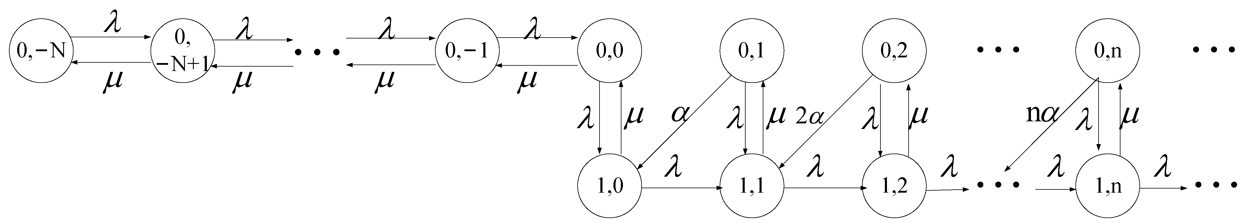
We consider a make-to-stock queueing system with a single producer and retrial customers. There is no waiting space in the system. Customers arrive in the system according to a Poisson process based on the parameter $\lambda$. When the customer arrives in the system, if some inventory of the product is available, the waiting time of a customer is zero; if the product is out of stock and the production server is idle, the customer is served immediately, and the time of the production server produces a unit of product accords to an exponential distribution with rate $\mu$; if the production server is busy, the customer joins in a retrial queue and becomes a repeat customer. Each repeat customer repeats their demand after an exponential amount of time with rate $\alpha$, independently of other customers, until they have been served. Customers are, thus, not served according to a first-come-first-serve strategy. Upon the completion of the service, each customer obtains a unit of the product. The maximum capacity of the stock is N. In general, we suppose that the inter-arrival time, production time, and the retrial time of each customer are mutually independent.

Let $N\left(t\right)$ be the queue length of customers or products at time t. $N\left(t\right)>0$ means that there are customers in the retrial queue, and $N\left(t\right)<0$ means that there are products in the system. $N\left(t\right)=0$ implies that there is neither a customer in the queue nor a product in the inventory at time t. Thus, it is impossible to have both customers and products in our model. $I\left(t\right)=1$ indicates that the production server is serving a customer (is busy), and $I\left(t\right)=0$ indicates that the production server is not servicing a customer (is idle) at time t. Therefore, $\left\{\right(I\left(t\right),N\left(t\right)\left)\right\}$ constitutes a two-dimensional (2D) Markovian chain with state space $\left\{\right(i,n):i=0,1;n=-N,-N+1,\cdots ,0,1,\cdots \}$. The corresponding transition rate diagram is shown in Figure 1.

After being served, each customer gains a profit R and incurs a cost $h_1$ for purchasing a unit of the product. The waiting cost of a customer for a unit time is $C_1$, while the storage cost of a unit of the product per unit time is $C_2$.

We study two different cases. The almost observable case is one in which the customers know only the state of the production server, while the unobservable case is one in which the customers do not know the length of the queues of customers and products or the state of the server.

3. Almost Observable Case

We now study the equilibrium strategies of customers and the expected cost of the entire system in the almost observable case, in which customers know only the state of the production server. Upon arrival into the system, customers join the system without hesitation and occupy the server if the production server is idle or there are products available in inventory. However, if the production server is already serving a customer when another arrives, the latter decides to join the retrial queue, according to probability q, or balk, according to probability $1-q$. If $\lambda <\mu$, the system is stable.

We give the steady-state probability ${\pi }_{i,j}$ of state $(i,j)$ and the particle probability-generating functions $P_0\left(s\right)={\sum }_{i=0}^{\infty }{\pi }_{0,i}{s}^i$, $P_1\left(s\right)={\sum }_{i=0}^{\infty }{\pi }_{1,i}{s}^i$ (see Lemma 1).

Lemma 1. 

The steady-state probability and particle probability-generating functions in the almost observable case are given as follows:

$$\begin{array}{ccc}\hfill {\pi }_{0,-N}& =& \frac{{(1-q\rho )}^{\frac{\lambda }{\alpha }+1}(1-\rho )}{{(1-q\rho )}^{\frac{\lambda }{\alpha }+1}(1-{\rho }^N)+{\rho }^N-{\rho }^{N+1}q-{\rho }^{N+2}+{\rho }^{N+2}q};\hfill \\ \hfill {\pi }_{0,i}& =& {\rho }^{i+N}{\pi }_{0,-N},-N+1\le i\le 0;\hfill \\ \hfill {\pi }_{0,i}& =& {\left(\frac{\lambda q}{\alpha \mu }\right)}^i\frac{{\prod }_{j=0}^{i-1}(\lambda +j\alpha )}{i!}{\pi }_{0,0},i\ge 1;\hfill \\ \hfill {\pi }_{1,i}& =& \frac{1}{\mu }{\left(\frac{\lambda q}{\alpha \mu }\right)}^i\frac{{\prod }_{j=0}^i(\lambda +j\alpha )}{i!}{\pi }_{0,0},i\ge 0;\hfill \\ \hfill P_0\left(s\right)& =& \frac{1}{{(1-q\rho s)}^{\frac{\lambda }{\alpha }}}{\pi }_{0,0};\hfill \\ \hfill P_1\left(s\right)& =& \frac{\rho }{{(1-q\rho s)}^{\frac{\lambda }{\alpha }+1}}{\pi }_{0,0}.\hfill \end{array}$$

Proof. 

We can obtain the balance equations from Figure 2.

$$\begin{array}{ccc}\hfill \lambda {\pi }_{0,-N}& =& \mu {\pi }_{0,-N+1};\hfill \end{array}$$

(1)

$$\begin{array}{ccc}(\lambda +\mu ){\pi }_{0,i}\hfill & =& \lambda {\pi }_{0,i-1}+\mu {\pi }_{0,i+1},-N+1\le i\le -1;\hfill \end{array}$$

(2)

$$\begin{array}{ccc}\hfill (\lambda +\mu ){\pi }_{0,0}& =& \lambda {\pi }_{0,-1}+\mu {\pi }_{1,0};\hfill \end{array}$$

(3)

$$\begin{array}{ccc}\hfill (\lambda +i\alpha ){\pi }_{0,i}& =& \mu {\pi }_{1,i},i\ge 1;\hfill \end{array}$$

(4)

$$\begin{array}{ccc}\hfill (\lambda q+\mu ){\pi }_{1,0}& =& \lambda {\pi }_{0,0}+\alpha {\pi }_{0,1};\hfill \end{array}$$

(5)

$$\begin{array}{ccc}\hfill (\lambda q+\mu ){\pi }_{1,i}& =& \lambda q{\pi }_{1,i-1}+\lambda {\pi }_{0,i}+(i+1)\alpha {\pi }_{0,i+1},i\ge 1.\hfill \end{array}$$

(6)

By substituting (4) into (6), we obtain

$$\begin{array}{c}\hfill {\pi }_{1,i}=\frac{\lambda +i\alpha }{\mu }{\pi }_{0,i},i\ge 1.\end{array}$$

By following with (6), we then have

$$\begin{array}{c}\hfill \lambda q(\lambda +i\alpha ){\pi }_{0,i}-(i+1)\alpha \mu {\pi }_{0,i+1}=\lambda q(\lambda +(i-1)\alpha ){\pi }_{0,i-1}-i\mu \alpha {\pi }_{0,i},i\ge 1.\end{array}$$

By using (3) and (5), we can then obtain

$$\begin{array}{c}\hfill \lambda q(\lambda +i\alpha ){\pi }_{0,i}-(i+1)\alpha \mu {\pi }_{0,i+1}=0,i\ge 1.\end{array}$$

Therefore,

$$\begin{array}{ccc}\hfill {\pi }_{0,i}& =& \hfill \frac{\lambda q(\lambda +(i-1\left)\alpha \right)}{i\alpha \mu }{\pi }_{0,i-1}={\left(\frac{\lambda q}{\alpha \mu }\right)}^i\frac{{\prod }_{j=0}^{i-1}(\lambda +j\alpha )}{i!}{\pi }_{0,0},i\ge 1.\hfill \\ \hfill {\pi }_{1,i}& =& \hfill \frac{\lambda +i\alpha }{\mu }{\pi }_{0,i}=\frac{1}{\mu }{\left(\frac{\lambda q}{\alpha \mu }\right)}^i\frac{{\prod }_{j=0}^i(\lambda +j\alpha )}{i!}{\pi }_{0,0},i\ge 0.\hfill \end{array}$$

By using (1) and (2), we obtain

$$\begin{array}{c}\hfill {\pi }_{0,i}={\rho }^{i+N}{\pi }_{0,-N},-N+1\le i\le -1,{\pi }_{0,0}={\rho }^N{\pi }_{0,-N}.\end{array}$$

Let $P_0\left(s\right)={\sum }_{i=0}^{\infty }{\pi }_{0,i}{s}^i$ and $P_1\left(s\right)={\sum }_{i=0}^{\infty }{\pi }_{1,i}{s}^i$.

By using the classical binomial formula, we can then obtain

$$\begin{array}{ccc}& & \hfill P_0\left(s\right)=\frac{1}{{(1-q\rho s)}^{\frac{\lambda }{\alpha }}}{\pi }_{0,0};\hfill \\ & & \hfill P_1\left(s\right)=\frac{\rho }{{(1-q\rho s)}^{\frac{\lambda }{\alpha }+1}}{\pi }_{0,0}.\hfill \end{array}$$

By using the normalized condition,

$$\begin{array}{c}\hfill {\displaystyle \sum _{i=-N}^{-1}}{\pi }_{0,i}+P_1\left(1\right)+P_0\left(1\right)=1\end{array}$$

we obtain

$$\begin{array}{ccc}\hfill {\pi }_{0,-N}& =& \hfill \frac{{(1-q\rho )}^{\frac{\lambda }{\alpha }+1}(1-\rho )}{{(1-q\rho )}^{\frac{\lambda }{\alpha }+1}(1-{\rho }^N)+{\rho }^N-{\rho }^{N+1}q-{\rho }^{N+2}+{\rho }^{N+2}q}.\hfill \end{array}$$

□

The mean number of customers $\mathbb{E}{N}_c$ in the retrial queue is

$$\begin{array}{ccc}\mathbb{E}{N}_c& =& \frac{d}{ds}{P}_0\left(s\right){{|}_{s=1}+\frac{d}{ds}{P}_1\left(s\right)|}_{s=1}\hfill \\ & =& \frac{(\frac{\lambda }{\alpha }(1-q\rho )+(\frac{\lambda }{\alpha }+1)\rho )({\rho }^{N+1}q-{\rho }^{N+2}q)}{(1-q\rho )\left({(1-q\rho )}^{\frac{\lambda }{\alpha }+1}(1-{\rho }^N)+{\rho }^N-{\rho }^{N+1}q-{\rho }^{N+2}+{\rho }^{N+2}q\right)},\hfill \end{array}$$

(7)

Therefore, when the server is busy, we achieve the mean waiting time of customers, which is $E\left(W_c\right|I\left(t\right)=1)$:

$$\begin{array}{c}\hfill E\left(W_c\right|I\left(t\right)=1)=\frac{E{N}_c}{{\lambda }_r}=\frac{\frac{\rho }{\alpha }(1-q)+\frac{1}{\alpha }+\frac{1}{\mu }}{1-q\rho }.\end{array}$$

where ${\lambda }_r$ is the effective arrival rate of customers,

$$\begin{array}{c}\hfill {\lambda }_r=\lambda q{P}_1\left(1\right)=\lambda q\frac{{\rho }^{N+1}(1-\rho )}{{(1-q\rho )}^{\frac{\lambda }{\alpha }+1}(1-{\rho }^N)+{\rho }^N-{\rho }^{N+1}q-{\rho }^{N+2}+{\rho }^{N+2}q}.\end{array}$$

The mean utility of a customer $U_c\left(q\right)$ is

$$\begin{array}{c}\hfill U_c\left(q\right)=R-h_1-C_{1}E\left(W_c\right|I\left(t\right)=1)=R-h_1-C_1\frac{E{N}_c}{{\lambda }_r}=R-h_1-C_1\frac{\frac{\rho }{\alpha }(1-q)+\frac{1}{\alpha }+\frac{1}{\mu }}{1-q\rho }.\end{array}$$

If the server is already serving a customer as another arrives in the almost observable case, the latter decides to join the retrial queue, according to probability $q_e$, or balk, according to probability $1-q_e$. Then, the equilibrium strategy for the customer is their joining probability: $q_e$. We can then provide the customer equilibrium strategy by using Theorem 1.

Theorem 1. 

When the production server is busy, the customers’ equilibrium strategy in the almost observable case, which is as follows:

$$\begin{array}{c}{q}_e=\left\{\begin{array}{cc}\hfill 0,\hfill & \mathit{if}R\le h_1+C_1(\frac{\rho }{\alpha }+\frac{1}{\alpha }+\frac{1}{\mu });\hfill \\ \hfill q_e^{*},\hfill & \mathit{if}{h}_1+C_1(\frac{\rho }{\alpha }+\frac{1}{\alpha }+\frac{1}{\mu })<R<h_1+C_1\frac{\frac{1}{\alpha }+\frac{1}{\mu }}{1-\rho };\hfill \\ \hfill 1,\hfill & \mathit{if}R\ge h_1+C_1\frac{\frac{1}{\alpha }+\frac{1}{\mu }}{1-\rho },\hfill \end{array}\right.\end{array}$$

where $q_e^{*}=\frac{\frac{\rho }{\alpha }+\frac{1}{\alpha }+\frac{1}{\mu }-\frac{R-p_1}{C_1}}{\frac{\rho }{\alpha }-\frac{R-p_1}{C_1}\rho }$.

Proof. 

We can show that $U_c\left(q\right)$ is a decreasing function of q.

(1)

From the first case $R\le h_1+C_1(\frac{\rho }{\alpha }+\frac{1}{\alpha }+\frac{1}{\mu })$, we obtain $U_c\left(q\right)\le 0$. Then, the best choice for the customer is to balk, such that $q_e=0$.

(2)

From the second case $h_1+C_1(\frac{\rho }{\alpha }+\frac{1}{\alpha }+\frac{1}{\mu })<R<h_1+C_1\frac{\frac{1}{\alpha }+\frac{1}{\mu }}{1-\rho }$, we know that the function $U_c\left(q\right)=0$ has a unique solution for $q\in (0,1)$. Therefore, we can compute $q_e*=\frac{\frac{\rho }{\alpha }+\frac{1}{\alpha }+\frac{1}{\mu }-\frac{R-h_1}{C_1}}{\frac{\rho }{\alpha }+\frac{R-h_1}{C_1}\rho }$.

(3)

From the third case $R\ge h_1+C_1\frac{\frac{1}{\alpha }+\frac{1}{\mu }}{1-\rho }$, we obtain $U_c\left(q\right)\ge 0$; thus, the profits of customers are always positive. Therefore, their equilibrium strategy is $q_e=1$.

□

The mean number of products is

$$\begin{array}{ccc}\mathbb{E}{N}_T& =& {\displaystyle \sum _{i=-N}^{-1}}(-i){\pi }_{0,i}=\left(N-\frac{\rho (1-{\rho }^N)}{1-\rho }\right)\frac{{\pi }_{0,-N}}{1-\rho }\hfill \\ & =& \frac{(N(1-\rho )-\rho (1-{\rho }^N)){(1-q\rho )}^{\frac{\lambda }{\alpha }+1}}{(1-\rho )\left({(1-q\rho )}^{\frac{\lambda }{\alpha }+1}(1-{\rho }^N)+{\rho }^N-{\rho }^{N+1}q-{\rho }^{N+2}+{\rho }^{N+2}q\right)}.\hfill \end{array}$$

(8)

By using (7) and (8), we obtain the expected cost function of the entire system $S_{ob}\left(N\right)$.

$$\begin{array}{ccc}{S}_{ob}\left(N\right)& =& C_1\mathbb{E}{N}_c+C_2\mathbb{E}{N}_T\hfill \\ & =& C_1\frac{(\frac{\lambda }{\alpha }(1-q\rho )+(\frac{\lambda }{\alpha }+1)\rho )({\rho }^{N+1}q-{\rho }^{N+2}q)}{(1-q\rho )\left({(1-q\rho )}^{\frac{\lambda }{\alpha }+1}(1-{\rho }^N)+{\rho }^N-{\rho }^{N+1}q-{\rho }^{N+2}+{\rho }^{N+2}q\right)}\hfill \\ & +& C_2\frac{(N(1-\rho )-\rho (1-{\rho }^N)){(1-q\rho )}^{\frac{\lambda }{\alpha }+1}}{(1-\rho )\left({(1-q\rho )}^{\frac{\lambda }{\alpha }+1}(1-{\rho }^N)+{\rho }^N-{\rho }^{N+1}q-{\rho }^{N+2}+{\rho }^{N+2}q\right)}\hfill \\ & =& \frac{C_1{(1-\rho )}^2(\frac{\lambda }{\alpha }(1-q\rho )+(\frac{\lambda }{\alpha }+1)\rho )q{\rho }^{N+1}+C_2\left((N(1-\rho )-\rho (1-{\rho }^N)){(1-q\rho )}^{\frac{\lambda }{\alpha }+2}\right)}{(1-q\rho )\left((1-\rho )\left({(1-q\rho )}^{\frac{\lambda }{\alpha }+1}(1-{\rho }^N)+{\rho }^N-{\rho }^{N+1}q-{\rho }^{N+2}+{\rho }^{N+2}q\right)\right)}.\hfill \end{array}$$

We can then obtain the optimal inventory level to minimize the expected cost function of the entire system. However, because the first- and second-order derivatives of N are complex, it is difficult for us to obtain the properties of $S_{ob}\left(N\right)$. Thus, we studied the optimal inventory level in the almost observable case through numerical experiments.

4. Unobservable Case

In this section, we consider the equilibrium strategies of customers and the expected cost of the entire system in the unobservable case. In this case, the customers do not know the state of the production server, the number of products in the inventory, and the length of the customer queue. When customers arrive in the system, they decide to join the system, according to probability q, or balk, according probability $1-q$ (Figure 3).

The steady-state probability of state $(i,j)$ is ${\pi }_{i,j}^{un}$, and $P_0^{un}\left(s\right)={\sum }_{i=0}^{\infty }{\pi }_{0,i}^{un}{s}^i$ and $P_1^{un}\left(s\right)={\sum }_{i=0}^{\infty }{\pi }_{1,i}^{un}{s}^i$ are the particle probability-generating functions in the unobservable case.

Lemma 2. 

The steady-state probabilities and partial probability-generating functions in the unobservable case are given as follows:

$$\begin{array}{ccc}\hfill {\pi }_{0,-N}^{un}& =& \frac{{(1-{\rho }_1)}^{\frac{{\lambda }_1}{\alpha }+2}}{{(1-{\rho }_1)}^{\frac{{\lambda }_1}{\alpha }+1}(1-{\rho }_1^N)+{\rho }_1^N(1-{\rho }_1)},\hfill \\ \hfill {\pi }_{0,i}^{un}& =& {\left(\frac{{\lambda }_1}{\alpha \mu }\right)}^i\frac{{\prod }_{j=0}^{i-1}({\lambda }_1+j\alpha )}{i!}{\pi }_{0,0}^{un},i\ge 1,\hfill \\ \hfill {\pi }_{1,i}^{un}& =& \frac{1}{\mu }{\left(\frac{{\lambda }_1}{\alpha \mu }\right)}^i\frac{{\prod }_{j=0}^i({\lambda }_1+j\alpha )}{i!}{\pi }_{0,0}^{un},i\ge 0,\hfill \\ \hfill {\pi }_{0,i}^{un}& =& {\rho }_1^{i+N}{\pi }_{0,-N}^{un},-N+1\le i\le 0,\hfill \\ \hfill P_0^{un}\left(s\right)& =& \frac{1}{{(1-{\rho }_{1}s)}^{\frac{{\lambda }_1}{\alpha }}}{\pi }_{0,0}^{un},\hfill \\ \hfill P_1^{un}\left(s\right)& =& \frac{{\rho }_1}{{(1-{\rho }_{1}s)}^{\frac{{\lambda }_1}{\alpha }+1}}{\pi }_{0,0}^{un},\hfill \end{array}$$

where ${\lambda }_1=\lambda q$ and ${\rho }_1=\frac{{\lambda }_1}{\mu }$.

Proof. 

The proof is similar to that of Lemma 1; therefore, we omit it here. □

In the following Theorem 9, we study the mean waiting time of customers in the unobservable case. We obtain the expected waiting time of customers by a general method in queueing models.

Theorem 2. 

The mean waiting time of customers $E{W}_c^{un}\left(q\right)$ is given as follows:

$$\begin{array}{c}\hfill E{W}_c^{un}\left(q\right)=\frac{{\lambda }_1+\alpha }{({(1-{\rho }_1)}^{\frac{{\lambda }_1}{\alpha }+1}(1-{\rho }_1^N)+{\rho }_1^N(1-{\rho }_1))\mu \alpha }.\end{array}$$

(9)

Proof. 

When a customer joins the system, if the state of the system is $(0,k),-N<k<0$, the waiting time of the customer is zero; if the state of the system is $(0,k),k\ge 0$, the waiting time of the customer is $\frac{1}{\mu }$; if the state of the system is $(1,k)$, the waiting time of the customer is $T(1,k)$, where

$$\begin{array}{ccc}T(1,k)& =& \frac{k}{2\mu -{\lambda }_1}+\frac{{\lambda }_1+2\alpha +2\mu }{\alpha (2\mu -{\lambda }_1)}+\frac{1}{\mu }\hfill \\ & =& \frac{k}{2\mu -{\lambda }_1}+\frac{\mu {\lambda }_1+4\alpha \mu +2{\mu }^2-\alpha {\lambda }_1}{\alpha \mu (2\mu -{\lambda }_1)}.\hfill \end{array}$$

Therefore, we obtain the mean customer waiting time: $E{W}_c^{un}$,

$$\begin{array}{ccc}E{W}_c^{un}& =& \frac{1}{\mu }{P}_0^{un}\left(1\right)+{\displaystyle \sum _{k=0}^{\infty }}T(1,k){\pi }_{1,k}\hfill \\ & =& \frac{1}{\mu }\frac{1}{{(1-{\rho }_1)}^{\frac{{\lambda }_1}{\alpha }}}{\pi }_{0,0}^{un}+\frac{\mu {\lambda }_1+4\alpha \mu +2{\mu }^2-\alpha {\lambda }_1}{\alpha \mu (2\mu -{\lambda }_1)}\frac{{\rho }_1}{{(1-{\rho }_1)}^{\frac{{\lambda }_1}{\alpha }+1}}{\pi }_{0,0}^{un}+\frac{1}{2\mu -{\lambda }_1}{\displaystyle \sum _{k=0}^{\infty }}k{\pi }_{1,k}^{un}\hfill \\ & =& \frac{\alpha (1-{\rho }_1)(2\mu -{\lambda }_1)+(\mu {\lambda }_1+4\alpha \mu +2{\mu }^2-\alpha {\lambda }_1){\rho }_1}{\alpha \mu (2\mu -{\lambda }_1){(1-{\rho }_1)}^{\frac{{\lambda }_1}{\alpha }+1}}{\pi }_{0,0}^{un}+\frac{1}{2\mu -{\lambda }_1}\frac{d{P}_1^{un}\left(s\right)}{ds}{|}_{s=1}\hfill \\ & =& \frac{2\alpha \mu +{\lambda }_1+\alpha {\lambda }_1+2\mu {\lambda }_1}{\alpha \mu (2\mu -{\lambda }_1){(1-{\rho }_1)}^{\frac{{\lambda }_1}{\alpha }+1}}{\pi }_{0,0}^{un}+\frac{1}{2\mu -{\lambda }_1}\frac{{\rho }_1^2(\frac{{\lambda }_1}{\alpha }+1)}{{(1-{\rho }_1)}^{\frac{{\lambda }_1}{\alpha }+2}}{\pi }_{0,0}^{un}\hfill \\ & =& \frac{(1-{\rho }_1)(2\alpha \mu +{\lambda }_1+\alpha {\lambda }_1+2\mu {\lambda }_1)+\alpha \mu {\rho }_1^2(\frac{{\lambda }_1}{\alpha }+1)}{{(1-{\rho }_1)}^{\frac{{\lambda }_1}{\alpha }+2}\mu \alpha (2\mu -{\lambda }_1)}{\pi }_{0,0}^{un}\hfill \\ & =& \frac{2\alpha \mu +2\mu {\lambda }_1-\alpha {\lambda }_1-{\lambda }_1^2}{{(1-{\rho }_1)}^{\frac{{\lambda }_1}{\alpha }+2}\mu \alpha (2\mu -{\lambda }_1)}{\pi }_{0,0}^{un}\hfill \\ & =& \frac{({\lambda }_1+\alpha ){\rho }_1^N}{({(1-{\rho }_1)}^{\frac{{\lambda }_1}{\alpha }+1}(1-{\rho }_1^N)+{\rho }_1^N(1-{\rho }_1))\mu \alpha }.\hfill \end{array}$$

□

In order to obtain the equilibrium strategy of a customer, we first study the monotonicity of $W_c^{un}\left(q\right)$ for the joining probability q.

Lemma 3. 

$W_c^{un}\left(q\right)$ is an increasing function of q.

Proof. 

Let $f=({\lambda }_1+\alpha ){\rho }_1^N,g={(1-{\rho }_1)}^{\frac{{\lambda }_1}{\alpha }+1}(1-{\rho }_1^N),h={\rho }_1^N(1-{\rho }_1)$. Then,

$$\begin{array}{c}\hfill \frac{dE{W}_c^{un}}{d{\lambda }_1}=\frac{1}{\mu \alpha }\frac{f^{\prime }(g+h)-f(g^{\prime }+h^{\prime })}{{(g+h)}^2}.\end{array}$$

(10)

where

$$\begin{array}{ccc}\hfill f^{\prime }& =& \hfill \frac{d\left(f\right)}{d{\lambda }_1}={\rho }_1^N+({\lambda }_1+\alpha )N{\rho }_1^{N-1}\frac{1}{\mu };\hfill \end{array}$$

(11)

$$\begin{array}{ccc}\hfill h^{\prime }& =& \hfill \frac{d\left(h\right)}{d{\lambda }_1}=-\frac{1}{\mu }{\rho }_1^N+\frac{1}{\mu }N{\rho }_1^{N-1}(1-{\rho }_1);\hfill \end{array}$$

(12)

$$\begin{array}{ccc}\hfill g^{\prime }& =& \hfill \frac{d\left(g\right)}{d{\lambda }_1}={\left[e^{ln{(1-{\rho }_1)}^{\frac{{\lambda }_1}{\alpha }+1}(1-{\rho }_1^N)}\right]}^{\prime }={\left[e^{\frac{{\lambda }_1}{\alpha }ln(1-{\rho }_1)+ln(1-{\rho }_1^N)}\right]}^{\prime }\hfill \end{array}$$

(13)

$$\begin{array}{ccc}& =& \hfill g\left[\frac{1}{\alpha }ln(1-{\rho }_1)+\frac{{\lambda }_1}{\alpha }\frac{-1}{\mu (1-{\rho }_1)}+\frac{-N{\rho }_1^{N-1}}{\mu (1-{\rho }_1^N)}\right].\hfill \end{array}$$

(14)

From (11) and (12), we obtain

$$\begin{array}{ccc}{f}^{\prime }h& =& \left\{{\rho }_1^N+({\lambda }_1+\alpha )N{\rho }_1^{N-1}\frac{1}{\mu }\right\}{\rho }_1^N(1-{\rho }_1)\hfill \\ & =& {\rho }_1^{2N}(1-{\rho }_1)+\frac{1}{\mu }({\lambda }_1+\alpha )N{\rho }^{2N-1}(1-{\rho }_1);\hfill \\ \hfill f{h}^{\prime }& =& ({\lambda }_1+\alpha ){\rho }_1^N(-\frac{{\rho }_1^N}{\mu }+\frac{1}{\mu }N{\rho }_1^{N-1}(1-{\rho }_1)).\hfill \end{array}$$

Therefore,

$$\begin{array}{c}\hfill f^{\prime }h-f{h}^{\prime }={\rho }_1^{2N}(1-{\rho }_1)+\frac{1}{\mu }({\lambda }_1+\alpha ){\rho }_1^{2N}>0.\end{array}$$

According to (11) and (14), we know that $f^{\prime }g>0$ and $f{g}^{\prime }<0$; thus, $\frac{dE{W}_c^{un}}{d{\lambda }_1}>0$. Therefore, $E{W}_c^{un}$ is an increasing function for q. □

The mean utility of a customer $U_c^{un}\left(q\right)$ is

$$\begin{array}{c}\hfill U_c^{un}\left(q\right)=R-h_1-C_1{W}_c^{un}\left(q\right).\end{array}$$

In the unobservable case, the customer decides to join the system, according to probability $q_{e1}$, or balk, according to probability $1-q_{e1}$, upon arrival. Then, the equilibrium strategy of a customer is $q_{e1}$. Theorem 3 shows the equilibrium strategy of a customer.

Theorem 3. 

The equilibrium strategy for the customer in the unobservable case is as follows:

$$\begin{array}{c}{q}_{e1}=\left\{\begin{array}{cc}\hfill 0,\hfill & \mathit{if}R<h_1+\frac{1}{\mu };\hfill \\ \hfill q_{e1}^{*},\hfill & \mathit{if}{h}_1+\frac{1}{\mu }<R<h_1+\frac{(\lambda +\alpha ){\rho }^N}{({(1-\rho )}^{\frac{\lambda }{\alpha }+1}(1-{\rho }^N)+{\rho }^N(1-\rho ))\mu \alpha };\hfill \\ \hfill 1,\hfill & \mathit{if}R>h_1+\frac{(\lambda +\alpha ){\rho }^N}{({(1-\rho )}^{\frac{\lambda }{\alpha }+1}(1-{\rho }^N)+{\rho }^N(1-\rho ))\mu \alpha }.\hfill \end{array}\right.\end{array}$$

where $q_{e1}^{*}$ is the unique solution to the function $U_c^{un}\left(q\right)=0$.

Proof. 

According to Lemma 3, $U_c^{un}\left(q\right)$ is a decreasing function of q.

(1)

From the first case, $U_c^{un}\left(0\right)\le 0$, we obtain $U_c^{un}\left(q\right)<0$ for $q\in [0,1]$ such that no customer enters the system because their profit is negative. Thus, $q_{e1}=0$.

(2)

From the second case, $U_c^{un}\left(0\right)<0<U_c^{un}\left(1\right)$, we know that $q_{e1}$ is the unique solution to the function $U_c^{un}\left(q\right)=0$ for $q\in (0,1)$.

(3)

From the third case, $U_c^{un}\left(1\right)\ge 0$, we obtain $U_c^{un}\left(q\right)>0$ for $q\in [0,1]$ such that each customer enters the system because their profit is positive. Thus, $q_{e1}=1$.

□

The expected number of products $E{N}_T^{un}$ is

$$\begin{array}{ccc}E{N}_T^{un}& =& {\displaystyle \sum _{i=-N}^{-1}}(-i){\pi }_{0,i}^{un}=\left(N-\frac{{\rho }_1(1-{\rho }_1^N)}{1-{\rho }_1}\right)\frac{{\pi }_{0,-N}^{un}}{1-{\rho }_1}\hfill \\ & =& \frac{(N(1-{\rho }_1)-{\rho }_1(1-{\rho }_1^N)){(1-{\rho }_1)}^{\frac{{\lambda }_1}{\alpha }}}{{(1-{\rho }_1)}^{\frac{{\lambda }_1}{\alpha }+1}(1-{\rho }_1^N)+{\rho }_1^N(1-{\rho }_1)}.\hfill \end{array}$$

(15)

By using Little’s law, (9), and (15), we obtain the expected cost function of the entire $S_{un}\left(N\right)$ system.

$$\begin{array}{ccc}{S}_{un}\left(N\right)& =& C_1{\lambda }_{1}E{W}_c^{un}+C_{2}E{N}_T^{un}\hfill \\ & =& C_1\frac{{\lambda }_1({\lambda }_1+\alpha ){\rho }_1^N}{({(1-{\rho }_1)}^{\frac{{\lambda }_1}{\alpha }+1}(1-{\rho }_1^N)+{\rho }_1^N(1-{\rho }_1))\mu \alpha }+C_2\left(N-\frac{{\rho }_1(1-{\rho }_1^N)}{1-{\rho }_1}\right)\frac{{\pi }_{0,-N}^{un}}{1-{\rho }_1}\hfill \\ & =& \frac{C_1{\lambda }_1({\lambda }_1+\alpha ){\rho }_1^N+C_2\mu \alpha (N(1-{\rho }_1)-{\rho }_1(1-{\rho }_1^N)){(1-{\rho }_1)}^{\frac{{\lambda }_1}{\alpha }}}{({(1-{\rho }_1)}^{\frac{{\lambda }_1}{\alpha }+1}(1-{\rho }_1^N)+{\rho }_1^N(1-{\rho }_1))\mu \alpha }.\hfill \end{array}$$

We can then achieve the optimal inventory level that minimizes the cost function $S_{un}\left(N\right)$. Because the expression for $S_{un}\left(N\right)$ is complex, it becomes challenging to determine the properties of the first- and second-order derivatives of N. Consequently, we analyzed the optimal inventory level through numerical experiments.

5. Numerical Experiments

We first studied the impact of key parameters (arrival rate: $\lambda$, production rate: $\mu$, retrial rate: $\alpha$, the profit of the customers: R, and the cost of waiting for a unit of time incurred by a customer: $C_1$) on the equilibrium strategy of a customer in both the almost observable and the unobservable cases. Additionally, we considered the influence of the inventory level, N, on the equilibrium strategy for the customer in the unobservable case. Furthermore, we also considered how the parameters $\mu ,\alpha ,q,$ and $C_1$ influence the optimal inventory levels in the two cases, and we provide a comparative analysis.

1. Equilibrium strategies of customers in the two cases

The equilibrium strategies of the customers in the almost observable and unobservable cases are $q_e$ and $q_{e1}$, respectively.

Table 1. Equilibrium strategies in the almost observable and the unobservable cases for $\mu =20$, $\alpha =4$, and $p_1=5,C_1=3,N=5$.

$\mathit{\lambda }$	15	16	$16.5$	17	$17.5$	18	$18.5$	19	$19.5$
$q_e$	1	1	$0.99$	$0.96$	$0.93$	$0.90$	$0.87$	$0.84$	$0.81$
$q_{e1}$	1	1	1	$0.99$	$0.96$	$0.94$	$0.91$	$0.89$	$0.87$

shows that the equilibrium strategies of the customers decrease in value as $\lambda$ increases in the two cases. This is because the customers know the historical rates of arrivals and the long waiting time (as more customers enter the system), thus making them less likely to enter the system.

The equilibrium strategies of customers in the two cases are decreasing functions of $\mu$ and $\alpha$, respectively, as shown in

Table 2. Equilibrium strategies in the almost observable and the unobservable case for $\lambda =15$, $\alpha =4$, $p_1=5$, $C_1=3$, $N=5$, and $R=10$.

$\mathit{\mu }$	16	17	18	19	20	21	22	23	24
$q_e$	$0.84$	$0.91$	$0.98$	1	1	1	1	1	1
$q_{ea}$	$0.89$	$0.95$	1	1	1	1	1	1	1

and

Table 3. Equilibrium strategies in the almost observable and the unobservable cases for $\lambda =18$, $\mu =20$, $p_1=5$, $C_1=3$, $R=10$, and $N=5$.

$\mathit{\alpha }$	2	3	4	5	6	7	8	9	10
$q_e$	$0.63$	$0.82$	$0.90$	$0.94$	$0.96$	$0.98$	$0.99$	1	1
$q_{e1}$	$0.83$	$0.90$	$0.94$	$0.96$	$0.98$	$0.99$	1	1	1

. This shows that if the production time or the retrial time decreases, the customers’ waiting times decrease as well; thus, more customers are willing to enter the system. The equilibrium strategies of the customers increase as R increases, as shown in

Table 4. Equilibrium strategies in the almost observable and the unobservable cases for $\lambda =18$, $\mu =20$, $\alpha =2$, $p_1=5$, $C_1=3$, and $N=3$.

R	8	9	10	11	12	13	14	15	16
$q_e$	0	$0.44$	$0.63$	$0.74$	$0.81$	$0.85$	$0.89$	$0.92$	$0.94$
$q_{e1}$	$0.71$	$0.78$	$0.83$	$0.87$	$0.90$	$0.92$	$0.94$	$0.95$	$0.96$

. The opposite outcome is obtained for $C_1$, as shown in

Table 5. Equilibrium strategies in the almost observable and the unobservable cases for $\lambda =18$, $\mu =20$, $\alpha =2$, $p_1=5$, $R=10$, and $N=3$.

${\mathit{C}}_1$	0	1	2	3	4	5	6	7	8
$q_e$	1	$0.99$	$0.83$	$0.63$	$0.37$	0	0	0	0
$q_{e1}$	1	1	$0.83$	$0.83$	$0.76$	$0.71$	$0.66$	$0.62$	$0.59$

.

Table 6. Equilibrium strategies in the almost observable and the unobservable cases for $\lambda =18$, $\mu =20$, $\alpha =2$, $p_1=5$, $C_1=3$, and $R=10$.

N	0	10	20	30	40	50	60	70	80
$q_{e1}$	$0.83$	$0.83$	$0.83$	$0.84$	$0.86$	$0.88$	$0.90$	$0.91$	$0.93$

shows that the equilibrium strategy for the customer increases for N in the unobservable case. Since incoming customers do not have information about the customers already in the queue and the state of the server, the higher the inventory level is, the higher the probability of incoming customers obtaining a product with zero service time. The mean waiting time of the customers decreases in this case. Therefore, customers are more likely to obtain products from the system. Table 1, Table 2, Table 3, Table 4, Table 5 and Table 6 show that the equilibrium strategy for the customer in the unobservable case is larger than that in the almost observable case, and this phenomenon is intuitive and understandable.

2. Optimal inventory levels in both cases

As shown in Figure 4 and Figure 5, the expected cost function of the entire system in the almost observable case is a concave function for the inventory level N. We can then obtain the optimal inventory level through numerical experiments. We can observe that the optimal inventory level decreases with the production rate, $\mu$ (see the above of Figure 4). If the producer can rapidly manufacture units, the manager can reduce the inventory level to reduce the storage cost of the product. The optimal inventory level decreases with $\alpha$ as well (see the below of Figure 4). The longer the retrial time is, the longer the waiting time for customers. Then, increasing the inventory level can reduce their expected waiting time. We know from Figure 5 that the optimal inventory level increases with the joining probability of the customer, q. This also holds for the waiting cost, $C_1$. These phenomena are reasonable. Moreover, when $C_1$ increases, the expected waiting time of customers increases as well, such that increasing the inventory level can reduce their expected waiting time.

From Figure 6 and Figure 7, we know that the effects of the parameters $\mu ,\alpha ,q,$ and $C_1$ on the inventory level in the unobservable case are the same as those in the almost observable case. However, the optimal inventory level in the almost observable case is greater than that in the unobservable case, see Figure 8. This is because there are products in the inventory or because the production server is idle upon customer arrival in the almost observable case, where they join the system without hesitation. Therefore, increasing the inventory level can reduce the expected cost of the entire system in the almost observable case.

6. Conclusions

In this article, we considered a make-to-stock queueing model with retrial customers. If customers are in the retrial queue, they become repeat customers. Each repeat customer repeats their demand after an exponential amount of time until they receive their requested service. We considered the equilibrium strategies of customers and the expected costs of the entire system in the almost observable and unobservable cases. Furthermore, we obtained the optimal inventory levels for both cases through numerical experiments. Additionally, we analyzed how the key parameters of the system influenced the strategic behaviors of the customers and the optimal inventory levels in both cases. Our results provide a reference for managers to appropriately stock their inventories and ensure the optimal operation of the production system.