Unit Maxwell-Boltzmann Distribution and Its Application to Concentrations Pollutant Data

Abstract

In the vast statistical literature, there are numerous probability distribution models that can model data from real-world phenomena. New probability models, nevertheless, are still required in order to represent data with various spread behaviors. It is a known fact that there is a great need for new models with limited support. In this study, a flexible probability model called the unit Maxwell-Boltzmann distribution, which can model data values in the unit interval, is derived by selecting the Maxwell-Boltzmann distribution as a base-line model. The important characteristics of the derived distribution in terms of statistics and mathematics are investigated in detail in this study. Furthermore, the inference problem for the mentioned distribution is addressed from the perspectives of maximum likelihood, method of moments, least squares, and maximum product space, and different estimators are obtained for the unknown parameter of the distribution. The derived distribution outperforms competitive models according to different fit tests and information criteria in the applications performed on four actual air pollutant concentration data sets, indicating that it is an effective model for modeling air pollutant concentration data.

1. Introduction

Volatile organic compounds (VOCs) are chemical pollutants that are frequently encountered in environments we breathe [1]. VOCs can be classified according to their volatility. The World Health Organization (WHO) classifies indoor pollutants into three categories: Very VOCs (VVOCs), VOCs, and Semi-VOCs (SVOCs). VVOCs are characterized by their extremely high volatility; this allows them to be predominantly found in the air in gaseous form rather than bound to materials or surfaces. Due to their high volatility, it is difficult to accurately measure VVOCs. On the other hand, SVOCs are less volatile and are more likely to be found in materials or surfaces rather than in the air. In indoor environments, the concentration of VVOCs is typically higher than SVOCs due to their high volatility and their tendency to be found in the air as a gas. Although it is difficult to accurately measure VVOCs, they play a significant role in indoor air quality. Personal exposure to VOCs, which are significant health concerns, has been evaluated by the U.S. Environmental Protection Agency (EPA) in various cities in the U.S. through research. In general, the EPA’s research underscores the importance of understanding different VOC categories according to volatility levels. Therefore, attempts to model the concentrations and ratios of these compounds are common in statistical science, and it is important to model them optimally. Aside from this, fraction evaluation is essential in a wide range of disciplines, from engineering to healthcare. Traditionally, distributions supported on the unit interval are crucial tools for modeling the behavior of such stochastic variables. Modeling and predicting such variables are possible, but model selection beyond traditional models is a must for establishing a base assumption as the measurements are limited to support (0, 1).

In this regard, researchers have proposed several statistical models for modeling the phenomena on the support (0, 1). The foundational work in this field includes the beta distribution, introduced by Bayes [2], which models these types of data. Subsequently, a variety of unit interval distributions have been explored, such as the unit distribution [3], the unit Johnson distribution [4], the four-parameter unit interval distribution [5], the double bounded Kumaraswamy distribution [6], the Topp-Leone distribution [7] by Topp and Leone, and the unit gamma distribution by Consul and Jain [8]. The alpha-unit model [9], which is based on the standard normal distribution, is another contemporary unitary distribution.

It is crucial to note that the constructions of the above-mentioned models employ several transformation methodologies. These are the cumulative distribution function and quantile transformation methodology, reciprocal transformation, exponentiation, conditional distribution methodology, the T-X family approach, and the epsilon function studied by Dombi et al. [10]. Upon using the above-mentioned strategies, researchers developed a limited number of unit interval distributions. To account for the vast range of data found in nature and measured within the unit interval, additional models are required. In recent years, researchers have made some advancements in introducing distributions that can statistically model phenomena that take values on a bounded support, thereby enriching the statistical literature with these new models. Some of these distributions include the quantile distribution by Smithson and Shou [11]; Altun and Hamedani [12]’s work unit log-X gamma distribution; Nakamura et al. [13]’s contribution regarding unit interval distribution; the unit inverse Guassian distribution by Ghitany et al. [14]; Mazucheli et al. [15,16,17]’s work on unit-Gompertz, unit-Lindley, and unit-Weibull distributions; and Gündüz et al. [18]’s work on the unit Johnson distribution. Additionally, Altun [19] studied the log-weighted exponential distribution, Biswas and Chakraborty [20] studied a new method for the construction of unit interval distribution, Afify et al. [21] worked on a unit interval distribution, Korkmaz and Korkmaz [22] studied unit log-log distribution, Fayomi et al. [23] studied the unit–power Burr X distribution, Krishna et al. [24] studied the unit Teissier Distribution using a conditional distribution approach, Biswas and Chakraborty [20] derived a number of unit distributions, and Bakouch et al. [25] derived the unit exponential distribution. These recent models have become important alternatives to the Beta distribution, a popular tool for modeling observations measured in the unit interval.

In this study, we used the Maxwell-Boltzmann distribution (MBD) for deriving a unit Maxwell-Boltzmann distribution (UMBD) by adopting the exponential transformation methodology. Hence, we used the UMBD to model and analyze the concentrations of pollutant data, which are the primary focus of this study.

The rest of this paper is organized as follows: Section 2 provides an overview of the Maxwell-Boltzmann distribution. Section 3 derives the unit Maxwell-Boltzmann distribution. Section 3 also investigates several characteristics of the unit Maxwell-Boltzmann distribution, such as survival, hazard rate function (hrf), reserved hazard rate function (rhrf), moment-generating functions, and its characterization. Section 4 investigates various estimators for estimating the unit Maxwell-Boltzmann distribution’s parameter. A Monte-Carlo simulation run is described in Section 5 to evaluate the efficiency of the estimators provided in this paper. In Section 6, several examples for data modeling using the UMBD are provided. These examples are presented to enable the evaluation of the UMBD’s performance in modeling real-world data and its effectiveness compared to alternatives. The work’s conclusin is provided in Section 7.

2. An Overview to Maxwell-Boltzmann Distribution

The MBD is a fundamental probability distribution in statistical physics that describes the distribution of the speeds or energies of particles in a gas at thermal equilibrium. The distribution of a particle’s kinetic energy can be found using MBD, and when the speed distribution is known, it can be associated with the particle’s speed using the formula $E=m{v}^2/2$, where $v$ is the speed and $m$ is the mass. The distribution function provides the probability of finding a particle with a certain speed or energy within the system. While this distribution is commonly used in physics and chemistry, it can also be used to model data that is measured on the positive real line. MBD is defined as follows.

Definition 1.

Let us assume that $X$ is a random variable following an MBD with parameter $\theta >0$, its pdf is represented by

$$g\left(x,\theta \right)=\sqrt{\frac{2}{\pi }}\frac{x^2}{{\theta }^3}\mathit{exp}\left(\frac{-x^2}{2{\theta }^2}\right),x>0$$

(1)

with the cdf is

$$G\left(x,\theta \right)=erf\left(\frac{x}{\sqrt{2}\theta }\right)-\sqrt{\frac{2}{\pi }}\frac{x}{\theta }\mathit{exp}\left(\frac{-x^2}{2{\theta }^2}\right),$$

(2)

and the hrf defined as

$$H\left(x\right)=\frac{x^2}{{\theta }^2\left(\theta e^{\frac{x^2}{2{\theta }^2}}\sqrt{\frac{\pi }{2}}\left(1-\mathrm{erf}\left(\frac{x}{\sqrt{2}\theta }\right)\right)+x\right)},$$

(3)

where $\theta$ is a positive-real valued shape parameter of the MBD and erf(.) implies the error function.

For further information on the error function, refer to Abramowitz and Stegun [26]. The hazard rate function of the MBD usually exhibits an increasing failure rate pattern for all of the parameter’s values. The pdf and cdf of the MBD are illustrated in Figure 1 for various parameter values.

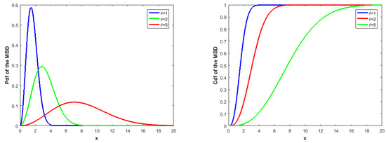
Figure 1. The pdf (left) and cdf (right) of the MBD for various values of $\theta$.

3. Unit Maxwell-Boltzmann Distribution and Its Principal Characteristics

The purpose of this section is to derive the pdf and cdf of the UMBD. As part of this section, we also examine statistically significant features of the UMBD, such as the hrf, rhrf, the moments, the moment generating function, the characteristic function, the skewness, and the kurtosis coefficients, as well as the mean, variance, and median.

Definition 2.

Let $X$ be a random variable from MBD with parameter $\theta >0$. Then, the pdf of the random variable $Y=e^{-X}$ is

$$f\left(y,\theta \right)=\frac{\sqrt{\frac{2}{\pi }}{\mathit{ln}}^2\left(\frac{1}{y}\right)e^{-\frac{{\mathit{ln}}^2\left(\frac{1}{y}\right)}{2{\theta }^2}}}{{\theta }^{3}y},0<y<1,$$

(4)

and the corresponding cdf is

$$F\left(y;\theta \right)=1-\frac{\sqrt{{\ln }^2\left(\frac{1}{y}\right)}\mathrm{erf}\left(\frac{\sqrt{{\ln }^2\left(\frac{1}{y}\right)}}{\sqrt{2}\theta }\right)}{\ln \left(\frac{1}{y}\right)}+\frac{\sqrt{\frac{2}{\pi }}\ln \left(\frac{1}{y}\right){\mathrm{e}}^{-\frac{{\ln }^2\left(\frac{1}{y}\right)}{2{\theta }^2}}}{\mathsf{\theta }},0<y<1,$$

(5)

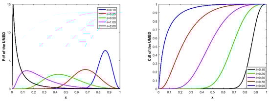
where $\theta$ is a positive real-valued parameter. The pdf and cdf of the UMBD are plotted in Figure 2 to provide information on the formal behavior of the model for a range of θ parameter values. The UMBD is a useful model for handling data with left- or right-skewed distributions that are defined on support (0, 1), as shown in Figure 2.

Figure 2. The pdf (left) and cdf (right) of the UMBD for various values of the $\theta$.

Next, we examine the UMBD’s characteristics, including its survival function, hrf, rhrf, mode, moments, variance, kurtosis and skewness coefficients, and characteristic and moment-generating functions.

Assume Y is a UMBD-distributed random variable with parameter $\theta .$ The UMBD’s survival function $S_Y\left(y\right)$, $\left(y\in \left(0,1\right)\right)$, when pdf (4) and cdf (5) are taken into account, is:

$$\begin{array}{ll}{S}_Y\left(y\right)& =1-F_Y\left(y,\theta \right)\\ & =\frac{\sqrt{{\ln }^2\left(\frac{1}{y}\right)}\mathrm{erf}\left(\frac{\sqrt{{\ln }^2\left(\frac{1}{y}\right)}}{\sqrt{2}\theta }\right)}{\ln \left(\frac{1}{y}\right)}-\frac{\sqrt{\frac{2}{\pi }}\ln \left(\frac{1}{y}\right)e^{-\frac{{\ln }^2\left(\frac{1}{y}\right)}{2{\theta }^2}}}{\theta }.\end{array}$$

(6)

By the definition of the hrf, the hrf of UMBD is

$$H\left(y\right)=\frac{{\ln }^2\left(\frac{1}{y}\right)}{\sqrt{\frac{\pi }{2}}{\theta }^{3}y{\mathrm{e}}^{\frac{{\ln }^2\left(\frac{1}{y}\right)}{2{\theta }^2}}\mathrm{erf}\left(\frac{\ln \left(\frac{1}{y}\right)}{\sqrt{2}\theta }\right)-{\mathsf{\theta }}^2\mathrm{y}\ln \left(\frac{1}{y}\right)}$$

(7)

and reserved hazard rate of $Y$ is

$$\xi \left(y\right)=\frac{\sqrt{\frac{\pi }{2}}{\ln }^2\left(\frac{1}{y}\right)}{{\theta }^2\left(\mathsf{\theta }\mathrm{y}{\mathrm{e}}^{\frac{{\ln }^2\left(\frac{1}{\mathrm{y}}\right)}{2{\theta }^2}}\left(1-\mathrm{erf}\left(\frac{\ln \left(\frac{1}{y}\right)}{\sqrt{2}\theta }\right)\right)-\sqrt{\frac{\pi }{2}}y\ln \left(\frac{1}{y}\right)\right)}.$$

(8)

The hrf and rhrf of the UMBD are plotted in Figure 3 for various values of parameter $\theta$ to exemplify of their behavior:

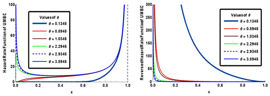
Figure 3. The hrf and rhrf of the UMBD for various values of $\theta$.

Figure 3 shows that the UMBD’s hrf is compatible with bathtub ($\theta \to 3\mathrm{o}\mathrm{r}\theta \ge 3$) or increasing forms ($\theta <3$), while its reverse hazard function decreases for all values of $\theta$.

Proposition 1.

If the random variable $Y$ follows the UMBD with parameter $\theta$, then H(y) satisfies

$$\frac{f\prime \left(y\right)}{f\left(y\right)}=\frac{H\prime \left(y\right)}{H\left(y\right)}-H\left(y\right).$$

(9)

Proof. 

Given that $Y$ is a continuous random variable and considering a general definition of the hrf and Equation (7), one can promptly write

$$\frac{H\prime \left(y\right)}{H\left(y\right)}=\frac{f^{\prime }\left(y\right)S\left(y\right)+f^2\left(x\right)}{{S\left(y\right)}^2}\frac{S\left(y\right)}{f\left(y\right)}=\frac{f\prime \left(y\right)}{f\left(y\right)}+H\left(y\right)$$

(10)

Hence, the proposition statement follows. □

Proposition 2.

Suppose a random variable $Y:\Omega \to (0,1)$ follows the UMBD with parameter $\theta$, and $H\left(y\right)$ is its hrf given by Equation (7). Then, the following equation holds.

$$\frac{H\prime \left(y\right)}{{\left(H\left(y\right)\right)}^2}=\frac{({(\mathit{ln}(\frac{1}{y}\left)\right)}^2-2{\theta }^2-{\theta }^{2}ln(\frac{1}{y}))(\theta erf[\frac{\mathit{ln}\left(\frac{1}{y}\right)}{\sqrt{2}\theta }]-e^{-\frac{{\left(\mathit{ln}\left(\frac{1}{y}\right)\right)}^2}{2{\theta }^2}}\sqrt{\frac{2}{\pi }}\mathit{ln}(\frac{1}{y}))}{e^{-\frac{{\left(\mathit{ln}\left(\frac{1}{y}\right)\right)}^2}{2{\theta }^2}}\sqrt{\frac{2}{\pi }}{\left(\mathit{ln}\left(\frac{1}{y}\right)\right)}^3}$$

(11)

Proof. 

Necessity: Given that $Y$ follows the UMBD $\left(\theta \right)$ with the probability density function $f\left(y\right)$ defined by Equation (4), one can express the logarithm of this pdf as follows:

$$\ln \left(f\left(y\right)\right)=\mathrm{l}\mathrm{n}\left(\sqrt{\frac{2}{\pi }}\right)+2\ln \left(\ln \left(\frac{1}{y}\right)\right)-\frac{{\left(\ln \left(\frac{1}{y}\right)\right)}^2}{2{\theta }^2}-\ln \left(y\right)-3\ln \left(\theta \right).$$

(12)

If the above equality is differentiated concerning $y$, the following is obtained:

$$\frac{f\prime \left(y\right)}{f\left(y\right)}=\frac{{\left(\mathrm{l}\mathrm{n}\right(\frac{1}{y}\left)\right)}^2-2{\theta }^2-{\theta }^2\mathrm{l}\mathrm{n}\left(\frac{1}{y}\right)}{y{\theta }^2\mathrm{l}\mathrm{n}\left(\frac{1}{y}\right)}.$$

(13)

Using this equation and considering Proposition 1, we can write

$$\frac{H\prime \left(y\right)}{H\left(y\right)}=\frac{{\left(\mathrm{l}\mathrm{n}\right(\frac{1}{y}\left)\right)}^2-2{\theta }^2-{\theta }^2\mathrm{l}\mathrm{n}\left(\frac{1}{y}\right)}{y{\theta }^2\mathrm{l}\mathrm{n}\left(\frac{1}{y}\right)}+\frac{{\mathrm{e}}^{-\frac{{\left(\mathrm{l}\mathrm{n}\right(\frac{1}{y}\left)\right)}^2}{2{\theta }^2}}\sqrt{\frac{2}{\pi }}{\left(\mathrm{l}\mathrm{n}\right(\frac{1}{y}\left)\right)}^2}{y{\theta }^2(\theta \mathrm{e}\mathrm{r}\mathrm{f}[\frac{\mathrm{l}\mathrm{n}\left(\frac{1}{y}\right)}{\sqrt{2}\theta }]-{\mathrm{e}}^{-\frac{{\left(\mathrm{l}\mathrm{n}\right(\frac{1}{y}\left)\right)}^2}{2{\theta }^2}}\sqrt{\frac{2}{\pi }}\mathrm{l}\mathrm{n}(\frac{1}{y}))}.$$

(14)

After some simplification, this equation is reduced to Equation (11).

Sufficiency: Given that Equation (11) holds, upon integration, we can express it as

$$\int \frac{H\prime \left(u\right)}{{\left(H\left(u\right)\right)}^2}du=\int \frac{({(\ln (\frac{1}{u}\left)\right)}^2-2{\theta }^2-{\theta }^2\ln (\frac{1}{u}))(\theta \mathrm{erf}[\frac{\ln \left(\frac{1}{u}\right)}{\sqrt{2}\theta }]-{\mathrm{e}}^{-\frac{{\left(\ln \left(\frac{1}{u}\right)\right)}^2}{2{\theta }^2}}\sqrt{\frac{2}{\pi }}\ln (\frac{1}{u}))}{{\mathrm{e}}^{-\frac{{\left(\ln \left(\frac{1}{u}\right)\right)}^2}{2{\theta }^2}}\sqrt{\frac{2}{\pi }}{\left(\ln \left(\frac{1}{u}\right)\right)}^3}du,$$

(15)

That is,

$$-\frac{1}{H\left(u\right)}=\frac{u{\theta }^2\left(\theta \mathrm{erf}\left[\frac{\ln \left(\frac{1}{u}\right)}{\sqrt{2}\theta }\right]-{\mathrm{e}}^{-\frac{{\left(\ln \left(\frac{1}{u}\right)\right)}^2}{2{\theta }^2}}\sqrt{\frac{2}{\pi }}\ln \left(\frac{1}{u}\right)\right)}{{\mathrm{e}}^{-\frac{{\left(\ln \left(\frac{1}{u}\right)\right)}^2}{2{\theta }^2}}\sqrt{\frac{2}{\pi }}{\left(\ln \left(\frac{1}{u}\right)\right)}^2}.$$

(16)

If Equation (16) is integrated from 0 to $y$, it is obtained that

$$-\ln \left(1-F\left(y\right)\right)=-\ln \left(\frac{\sqrt{{\ln }^2\left(\frac{1}{y}\right)}\mathrm{erf}\left(\frac{\sqrt{{\ln }^2\left(\frac{1}{y}\right)}}{\sqrt{2}\theta }\right)}{\ln \left(\frac{1}{y}\right)}-\frac{\sqrt{\frac{2}{\pi }}\ln \left(\frac{1}{y}\right)e^{-\frac{{\ln }^2\left(\frac{1}{y}\right)}{2{\theta }^2}}}{\theta }\right),$$

(17)

which after simplification yields

$$F\left(y\right)=1-\frac{\sqrt{{\ln }^2\left(\frac{1}{y}\right)}\mathrm{erf}\left(\frac{\sqrt{{\ln }^2\left(\frac{1}{y}\right)}}{\sqrt{2}\theta }\right)}{\ln \left(\frac{1}{y}\right)}+\frac{\sqrt{\frac{2}{\pi }}\ln \left(\frac{1}{y}\right)e^{-\frac{{\ln }^2\left(\frac{1}{y}\right)}{2{\theta }^2}}}{\theta },$$

(18)

whereby from the conditions $F\left(0\right)=0$ and $F\left(1\right)=1$. Thus, the proof is finished and the function $F\left(y\right)$ is verified as the cdf from the UMBD $\left(\theta \right)$. □

Lemma 3.

Suppose $r>0$ is an integer. The rth raw moment, ${\mu }_r$, of the UMBD$\left(\theta \right)$ is

$${\mu }_r=\left(e^{\frac{{\theta }^2{r}^2}{2}}\left({\theta }^2{r}^2+1\right)\mathit{erfc}\left(\frac{\theta r}{\sqrt{2}}\right)-\sqrt{\frac{2}{\pi }}\theta r\right).$$

(19)

Proof. 

Considering pdf (4) and following the definition of the rth moment, we have

$$\begin{array}{ll}{\mu }_r& =E\left(Y^r\right)=\underset{-\mathrm{\infty }}{\overset{\mathrm{\infty }}{\int }}{y}^{r}f\left(y,\theta \right)dy\\ & =\underset{0}{\overset{1}{\int }}{y}^r\frac{\sqrt{\frac{2}{\pi }}{\ln }^2\left(\frac{1}{y}\right)e^{-\frac{{\ln }^2\left(\frac{1}{y}\right)}{2{\theta }^2}}}{{\theta }^{3}y}dy\\ & =\left(e^{\frac{{\theta }^2{r}^2}{2}}\left({\theta }^2{r}^2+1\right)\mathrm{erfc}\left(\frac{\theta r}{\sqrt{2}}\right)-\sqrt{\frac{2}{\pi }}\theta r\right).\end{array}$$

(20)

Using Equation (20), the first two raw moments of the UMBD can be expressed as

$${\mu }_1=e^{\frac{{\theta }^2}{2}}\left({\theta }^2+1\right)\mathrm{erfc}\left(\frac{\theta }{\sqrt{2}}\right)-\sqrt{\frac{2}{\pi }},$$

(21)

$${\mu }_2=e^{2{\theta }^2}\left(4{\theta }^2+1\right)\mathrm{erfc}\left(\sqrt{2}\theta \right)-2\sqrt{\frac{2}{\mathsf{\pi }}}\theta$$

(22)

.

Thus, the variance of the UMBD is

$$\begin{gathered} Var\left(Y\right)={\mu }_2-{\mu }_1^2 \\ =-{\left(\sqrt{\frac{2}{\pi }}\theta -e^{\frac{{\theta }^2}{2}}\left({\theta }^2+1\right)\mathrm{erfc}\left(\frac{\theta }{\sqrt{2}}\right)\right)}^2+e^{2{\theta }^2}\left(4{\theta }^2+1\right)\mathrm{erfc}\left(\sqrt{2}\theta \right)-2\sqrt{\frac{2}{\mathsf{\pi }}}\theta . \end{gathered}$$

(23)

Furthermore, the moment generating function and the characteristic function of the UMBD are as follows:

$$\begin{array}{ll}{M}_Y\left(t\right)& =\underset{-\mathrm{\infty }}{\overset{\mathrm{\infty }}{\int }}{e}^{ty}f\left(y,\theta \right)dy\\ & ={\displaystyle \sum _{j=0}^{\mathrm{\infty }}}\frac{t^j}{j!}\underset{0}{\overset{1}{\int }}{y}^{j}f\left(y,\theta \right)dy\\ & ={\displaystyle \sum _{j=0}^{\mathrm{\infty }}}\frac{t^j}{j!}\left(e^{\frac{{\theta }^2{j}^2}{2}}\left({\theta }^2{j}^2+1\right)\mathrm{erfc}\left(\frac{\theta j}{\sqrt{2}}\right)-\sqrt{\frac{2}{\pi }}\theta j\right)\end{array}$$

(24)

and

$$\begin{array}{ll}{\varphi }_Y\left(t\right)& =\underset{-\mathrm{\infty }}{\overset{\mathrm{\infty }}{\int }}{e}^{ity}f\left(y,\theta \right)dy\\ & ={\displaystyle \sum _{j=0}^{\mathrm{\infty }}}\frac{(i{t)}^j}{j!}\left(e^{\frac{{\theta }^2{j}^2}{2}}\left({\theta }^2{j}^2+1\right)\mathrm{erfc}\left(\frac{\theta j}{\sqrt{2}}\right)-\sqrt{\frac{2}{\pi }}\theta j\right),\end{array}$$

(25)

respectively. □

Proposition 4.

The mode of UMBD is $e^{-\frac{1}{2}\theta \left(\sqrt{{\theta }^2+8}+\theta \right)}$.

Proof. 

By considering the pdf of the UMBD, we have

$$f^{\prime }\left(y,\theta \right)=\frac{d}{dy}f\left(y,\theta \right)=\frac{\frac{\ln \left(\frac{1}{y}\right)}{{\theta }^2}-\frac{2}{\ln \left(\frac{1}{y}\right)}-1}{y}f\left(y,\theta \right)=0.$$

(26)

Considering $f\left(y,\theta \right)\ne 0$ for $\forall y\in (0,1)$, we can write from (26) as

$$\frac{2}{\ln \left(\mathrm{y}\right)}-\frac{\ln \left(y\right)}{{\theta }^2}-1=0.$$

(27)

Hence, from the solution of the Equation (27) with respect to $y$, the mode of the UMBD is obtained as $e^{-\frac{1}{2}\theta \left(\sqrt{{\theta }^2+8}+\theta \right)}$. □

4. Inference

The goal of this section of the study is to investigate the solution to the problem of estimating the unknown parameter of the UMBD. Here, maximum likelihood, least-squares, weighted-least-squares, maximum spacing, and moments estimation techniques are employed to accomplish this aim.

Let $Y_1,Y_2,...,Y_n$ be a sample of an independently and identically distributed UMBD with a one-dimensional parameter $\theta$, and let $y_1,y_2,...,y_n$ represent a realization of it. The likelihood function $L(\theta ,y_1,y_2,...,y_n)$ is

$$L\left(\theta ,y_1,y_2,...,y_n\right)=\prod _{i=1}^n\frac{\sqrt{\frac{2}{\pi }}{\ln }^2\left(\frac{1}{y_i}\right)e^{-\frac{{\ln }^2\left(\frac{1}{y_i}\right)}{2{\theta }^2}}}{{\theta }^3{y}_i}$$

(28)

and the logarithmic likelihood function is

$$\begin{array}{ll}\mathrm{l}\mathrm{n}L\left(\theta ,y_1,y_2,\dots ,y_n\right)& =\frac{1}{2}\left(-\frac{{\sum }_{\mathrm{i}=1}^{\mathrm{n}}{\ln }^2\left(y_i\right)}{{\theta }^2}+4{\displaystyle \sum _{\mathrm{i}=1}^{\mathrm{n}}}\ln \left(\ln \left(y_i\right)\right)-2{\displaystyle \sum _{\mathrm{i}=1}^{\mathrm{n}}}\ln \left(y_i\right)-6\mathrm{n}\ln \left(\theta \right)\right)\\ & +\frac{1}{2}\left(n\ln \left(2\right)-n\ln \left(\pi \right)\right).\end{array}$$

(29)

The maximum likelihood estimator (MLE) for the $\theta$ can be obtained by the derivation of Equation (29) concerning $\theta$ and setting the resulting derivative as equal to zero. The Equation (29)’s derivative with respect to $\theta$ is

$$\frac{\delta \mathrm{l}\mathrm{n}L\left(\theta ,y_1,y_2,\dots ,y_n\right)}{\delta \theta }=\left(\frac{{\sum }_{i=1}^n{\ln }^2\left(y_i\right)}{{\theta }^3}-\frac{3n}{\theta }\right)=0.$$

(30)

Hence, from the solution of the Equation (30), we have the MLE of the parameter $\theta$ as

$$\widehat{\theta }=\sqrt{\frac{{\sum }_{i=1}^n{\ln }^2\left(y_i\right)}{3n}}.$$

(31)

The least-squares estimator (LSE) of the $\theta$ can be obtained by minimizing the utility function as

$$Q_{LSE}=\sum _{i=j}^n{\left(1-\frac{\sqrt{{\ln }^2\left(\frac{1}{y_{\left(j\right)}}\right)}\mathrm{erf}\left(\frac{\sqrt{{\ln }^2\left(\frac{1}{y_{\left(j\right)}}\right)}}{\sqrt{2}\theta }\right)}{\ln \left(\frac{1}{y_{\left(j\right)}}\right)}+\frac{\sqrt{\frac{2}{\pi }}\ln \left(\frac{1}{y_{\left(j\right)}}\right){\mathrm{e}}^{-\frac{{\ln }^2\left(\frac{1}{y_{\left(j\right)}}\right)}{2{\mathsf{\theta }}^2}}}{\theta }-P_j\right)}^2,$$

(32)

with respect to parameter $\theta$, where $y_{\left(1\right)},y_{\left(2\right)},\dots ,y_{\left(n\right)}$ and $\left(y_{\left(1\right)}<y_{\left(2\right)}<\cdots <y_{\left(n\right)}\right)$ are an order with the measurements $y_1,y_2,...,y_n$, and $P_j=\frac{j}{n+1}$. For further information about least squares estimation methodology, see Günay & Yilmaz [27]. Here, the utility function $Q_{LSE}$ includes nonlinear functions and it has to be solved using a numerical method. We use the “fmincon” routine of the Octave [28] for minimizing the $Q_{LSE}$ function.

Similarly to LSE, the weighted-LSE (WLSE) for $\theta$ is obtained by minimizing the utility function

$$Q_{WLSE}=\sum _{j=1}^n\frac{{\left(n+1\right)}^2\left(n+2\right)}{j\left(n-j+1\right)}{\left(1-\frac{\sqrt{{\ln }^2\left(\frac{1}{y_{\left(j\right)}}\right)}\mathrm{erf}\left(\frac{\sqrt{{\ln }^2\left(\frac{1}{y_{\left(j\right)}}\right)}}{\sqrt{2}\theta }\right)}{\ln \left(\frac{1}{y_{\left(j\right)}}\right)}+\frac{\sqrt{\frac{2}{\pi }}\ln \left(\frac{1}{y_{\left(j\right)}}\right){\mathrm{e}}^{-\frac{{\ln }^2\left(\frac{1}{y_{\left(j\right)}}\right)}{2{\mathsf{\theta }}^2}}}{\theta }-P_j\right)}^2.$$

(33)

To construct the maximum product space estimator (MPSE) of the parameter $\theta$, we have used the [27] steps for this aim and have the utility function

$$Q_{MPSE}={\sum }_{j=1}^{n+1}\mathrm{l}\mathrm{n}\left[F\left(y_{\left(j\right)},\theta \right)-F\left(y_{(j-1)},\theta \right)\right],$$

(34)

$$Q_{MPSE}=\sum _{j=1}^{n+1}\ln \left\{1-\frac{\sqrt{{\ln }^2\left(\frac{1}{y_{\left(\mathrm{j}\right)}}\right)}\mathrm{erf}\left(\frac{\sqrt{{\ln }^2\left(\frac{1}{y_{\left(j\right)}}\right)}}{\sqrt{2}\theta }\right)}{\ln \left(\frac{1}{y_{\left(j\right)}}\right)}+\frac{\sqrt{\frac{2}{\pi }}\ln \left(\frac{1}{y_{\left(j\right)}}\right){\mathrm{e}}^{-\frac{{\ln }^2\left(\frac{1}{y_{\left(j\right)}}\right)}{2{\theta }^2}}}{\theta }-\right.\left.\left(1-\frac{\sqrt{{\ln }^2\left(\frac{1}{y_{(j-1)}}\right)}\mathrm{erf}\left(\frac{\sqrt{{\ln }^2\left(\frac{1}{y_{(j-1)}}\right)}}{\sqrt{2}\theta }\right)}{\ln \left(\frac{1}{y_{(j-1)}}\right)}+\frac{\sqrt{\frac{2}{\pi }}\ln \left(\frac{1}{{y(}_{j-1)}}\right){\mathrm{e}}^{-\frac{{\ln }^2\left(\frac{1}{y_{(j-1)}}\right)}{2{\theta }^2}}}{\theta }\right)\right\}.$$

(35)

Subsequently, the objective function $Q_{MPSE}$ regarding parameter $\theta$ is numerically maximized to yield the MPSE of $\theta$. In the function $Q_{MPSE}$, $F\left(Y_{\left(0\right)},\theta \right)\equiv 0$, and $F\left(Y_{(n+1)},\theta \right)\equiv 1$. For maximizing the function $Q_{MPSE}$, one can use the “fmincon” function of the Octave [28].

Based on $y_1,y_2,\dots ,y_n$ observations and the first moment of the UMBD given by Equation (20), an estimator based on the method of moments for $\theta$ denoted as ${\widehat{\theta }}_{MOM}$ can be formally derived by solving the equation

$$\frac{1}{n}\sum _{i=1}^n{y}_i=e^{\frac{{\theta }^2}{2}}\left({\theta }^2+1\right)\mathrm{erfc}\left(\frac{\theta }{\sqrt{2}}\right)-\sqrt{\frac{2}{\pi }}$$

(36)

with respect to $\theta$. Thus, the method of moments estimator (MOME) of the parameter $\theta$ is obtained analytically as

$${\widehat{\theta }}_{MOM}=\frac{\sqrt{\pi }}{2n\sqrt{2}}\sum _{i=1}^n\ln \left(\frac{1}{y_i}\right).$$

(37)

5. Simulation Study

In this section, performance of the estimators MLE, LSE, WLSE, MPSE, and MOME are numerically assessed. Criteria MSE and bias are used to compare the above-mentioned estimators, and they are denoted as

$$MSE=\frac{1}{m}\sum _{i=1}^n{\left(\theta -{\widehat{\theta }}_i\right)}^2$$

(38)

and

$$Bias=\frac{1}{m}\sum _{i=1}^n{\widehat{\theta }}_i-\theta ,$$

(39)

respectively, where $m$ implies the repetition number of the simulation. Table 1, Table 2, Table 3 and Table 4 exhibit the results of the simulations based on 1000 replicates performed on the different sample sizes of n = 50, 100, 500, and 1000.

Table 1. Simulated results based on the different sample sizes for parameter $\theta =0.25$.

	$\mathit{n}=30$			$\mathit{n}=50$			$\mathit{n}=100$			$\mathit{n}=200$
Method	$\widehat{\mathit{\theta }}$	$\mathbf{Bias}\widehat{\mathit{\theta }}$	$\mathbf{MSE}\widehat{\mathit{\theta }}$	$\widehat{\mathit{\theta }}$	$\mathbf{Bias}\widehat{\mathit{\theta }}$	$\mathbf{MSE}\widehat{\mathit{\theta }}$	$\widehat{\mathit{\theta }}$	$\mathbf{Bias}\widehat{\mathit{\theta }}$	$\mathbf{MSE}\widehat{\mathit{\theta }}$	$\widehat{\mathit{\theta }}$	$\mathbf{Bias}\widehat{\mathit{\theta }}$	$\mathbf{MSE}\widehat{\mathit{\theta }}$
MLE	0.2491	0.0009	0.0002	0.2487	0.0013	0.0002	0.2498	0.0002	0.0001	0.2507	0.0007	0.0001
LSE	0.2510	0.0010	0.0003	0.2494	0.0006	0.0003	0.2512	0.0012	0.0002	0.2512	0.0012	0.0001
WLSE	0.2508	0.0008	0.0003	0.2493	0.0007	0.0003	0.2511	0.0011	0.0002	0.2509	0.0009	0.0001
MPSE	0.2493	0.0007	0.0002	0.2486	0.0014	0.0002	0.2499	0.0001	0.0001	0.2507	0.0007	0.0001
MOME	0.2501	0.0001	0.0003	0.2489	0.0011	0.0003	0.2507	0.0007	0.0002	0.2507	0.0007	0.0001

Table 2. Simulated results based on the different sample sizes for parameter $\theta =0.50$.

	$\mathit{n}=30$			$\mathit{n}=50$			$\mathit{n}=100$			$\mathit{n}=200$
Method	$\widehat{\mathit{\theta }}$	$\mathbf{Bias}\widehat{\mathit{\theta }}$	$\mathbf{MSE}\widehat{\mathit{\theta }}$	$\widehat{\mathit{\theta }}$	$\mathbf{Bias}\widehat{\mathit{\theta }}$	$\mathbf{MSE}\widehat{\mathit{\theta }}$	$\widehat{\mathit{\theta }}$	$\mathbf{Bias}\widehat{\mathit{\theta }}$	$\mathbf{MSE}\widehat{\mathit{\theta }}$	$\widehat{\mathit{\theta }}$	$\mathbf{Bias}\widehat{\mathit{\theta }}$	$\mathbf{MSE}\widehat{\mathit{\theta }}$
MLE	0.5007	0.0007	0.0013	0.5009	0.0009	0.0008	0.4957	0.0043	0.0004	0.4981	0.0019	0.0002
LSE	0.5019	0.0019	0.0015	0.5022	0.0022	0.0009	0.4970	0.0030	0.0004	0.4993	0.0007	0.0002
WLSE	0.5024	0.0024	0.0015	0.5028	0.0028	0.0009	0.4968	0.0032	0.0004	0.4989	0.0011	0.0002
MPSE	0.5017	0.0017	0.0013	0.5014	0.0014	0.0008	0.4959	0.0041	0.0004	0.4982	0.0018	0.0002
MOME	0.5005	0.0005	0.0013	0.5022	0.0022	0.0008	0.4962	0.0038	0.0004	0.4983	0.0017	0.0002

Table 3. Simulated results based on the different sample sizes for parameter $\theta =1.00$.

	$\mathit{n}=30$			$\mathit{n}=50$			$\mathit{n}=100$			$\mathit{n}=200$
Method	$\widehat{\mathit{\theta }}$	$\mathbf{Bias}\widehat{\mathit{\theta }}$	$\mathbf{MSE}\widehat{\mathit{\theta }}$	$\widehat{\mathit{\theta }}$	$\mathbf{Bias}\widehat{\mathit{\theta }}$	$\mathbf{MSE}\widehat{\mathit{\theta }}$	$\widehat{\mathit{\theta }}$	$\mathbf{Bias}\widehat{\mathit{\theta }}$	$\mathbf{MSE}\widehat{\mathit{\theta }}$	$\widehat{\mathit{\theta }}$	$\mathbf{Bias}\widehat{\mathit{\theta }}$	$\mathbf{MSE}\widehat{\mathit{\theta }}$
MLE	1.0084	0.0084	0.0085	0.9947	0.0053	0.0037	1.0003	0.0003	0.0018	0.9983	0.0017	0.0010
LSE	1.0100	0.0100	0.0097	0.9933	0.0067	0.0052	1.0003	0.0003	0.0023	1.0021	0.0021	0.0011
WLSE	1.0110	0.0110	0.0097	0.9930	0.0070	0.0052	1.0003	0.0003	0.0023	1.0011	0.0011	0.0011
MPSE	1.0077	0.0077	0.0088	0.9934	0.0066	0.0038	1.0003	0.0003	0.0018	0.9984	0.0016	0.0010
MOME	1.0079	0.0079	0.0088	0.9951	0.0049	0.0039	1.0002	0.0002	0.0020	0.9999	0.0001	0.0010

Table 4. Simulated results based on the different sample sizes for parameter $\theta =2.00$.

	$\mathit{n}=30$			$\mathit{n}=50$			$\mathit{n}=100$			$\mathit{n}=200$
Method	$\widehat{\mathit{\theta }}$	$\mathbf{Bias}\widehat{\mathit{\theta }}$	$\mathbf{MSE}\widehat{\mathit{\theta }}$	$\widehat{\mathit{\theta }}$	$\mathbf{Bias}\widehat{\mathit{\theta }}$	$\mathbf{MSE}\widehat{\mathit{\theta }}$	$\widehat{\mathit{\theta }}$	$\mathbf{Bias}\widehat{\mathit{\theta }}$	$\mathbf{MSE}\widehat{\mathit{\theta }}$	$\widehat{\mathit{\theta }}$	$\mathbf{Bias}\widehat{\mathit{\theta }}$	$\mathbf{MSE}\widehat{\mathit{\theta }}$
MLE	1.9925	0.0075	0.0184	2.0063	0.0063	0.0125	1.9966	0.0034	0.0059	1.9928	0.0072	0.0029
LSE	1.9965	0.0035	0.0179	2.0180	0.0180	0.0140	1.9989	0.0011	0.0081	1.9958	0.0042	0.0033
WLSE	1.9953	0.0047	0.0179	2.0187	0.0187	0.0140	1.9997	0.0003	0.0081	1.9953	0.0047	0.0033
MPSE	1.9866	0.0134	0.0180	2.0075	0.0075	0.0126	1.9972	0.0028	0.0059	1.9930	0.0070	0.0030
MOME	1.9902	0.0098	0.0178	2.0111	0.0111	0.0128	1.9997	0.0003	0.0062	1.9940	0.0060	0.0030

Based on the results provided in Table 1, Table 2, Table 3 and Table 4, it can be concluded that all estimates perform well in estimating parameter $\theta$ with sufficiently small bias and MSE values. Additionally, we ran another simulation to examine how the estimators perform asymptotically. We set the value of parameter $\theta$ as 1 without loss of generality. The bias and MSE values of each estimate are calculated for different sample sizes $n$ by 1000 simulations. The simulated results are displayed in Figure 4. One can see from Figure 4 that the bias and MSE values of the estimates decrease when the sample size $n$ increases. Therefore, it can be asserted that all estimates exhibit asymptotic consistency and are unbiased.

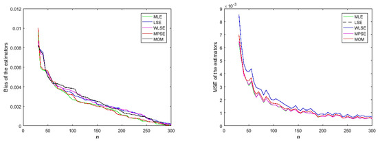
Figure 4. Bias and MSE of competitive methods.

6. Applications

Air pollution (Ap) is a multifaceted environmental problem that comes from various sources. The main sources of Ap include factories, refineries, vehicle emissions, energy production plants (especially those that rely on coal or oil), and other activities that release pollutants into the atmosphere [29]. Many of these pollutants are also sources of greenhouse gas emissions.

The health effects of Ap are significant; long-term exposure is linked to chronic conditions such as asthma, cardiovascular diseases, and premature death [30]. Major pollutants that cause such health problems include VOCs. In addition to affecting human health, Ap also affects agricultural productivity by disrupting plant biochemical reactions and causing soil degradation through acid rain [31].

In general, Ap can be considered as a global problem. Comprehensive strategies developed to overcome this problem and reduce sources of Ap contribute to the health of the environment and quality of life in the long term by offering a win-win strategy for reducing its effects on health and the environment and increasing general well-being and sustainability.

We have studied four environmental datasets for modeling harmful air pollutant contents like carbon monoxide (CO), sulfate particles and benzo(a)pyrene that are monitored on a continuous basis. Concentrations of these pollutants are reported once every hour, 24 h a day, and 365 days a year.

6.1. Competing Models

In this section, we compare the fits of the UMBD with the unit Topp Leone (UTL), unit log-Lindley (ULL), unit log-weighted exponential (ULWE), and unit Kumerswamy (UKw) distributions. All of these distributions are used for modeling bounded data. To reveal the potential of the UMBD model, these models are compared through analyses conducted on four environmental data sets. The pdfs of competing models are expressed in Table 5.

Table 5. Competing models with distribution functions.

Distribution	Distribution Function	Domain of Function	Reference
UTL	$x^{\theta }{\left(2-x\right)}^{\theta }$	${\mathrm{I}}_{\left(0,1\right)}\left(x\right)$, θ > 0	[32]
ULL	$\frac{x^{\theta }{\left(1+\theta (\lambda -\mathrm{l}\mathrm{o}\mathrm{g}(x\left)\right)\right)}^{\theta }}{1+\theta \lambda }$	${\mathrm{I}}_{\left(0,1\right)}\left(x\right)$, θ > 0, λ > 0	[33]
ULWE	$\frac{(1+\theta )(x^{\lambda }-\frac{x^{\left(1+\theta \right)\lambda }}{1+\theta })}{\theta }$	${\mathrm{I}}_{\left(0,1\right)}\left(x\right)$, θ > 0, λ > 0	[19]
UKw	$1-{\left(1-x^{\theta }\right)}^{\lambda }$	${\mathrm{I}}_{\left(0,1\right)}\left(x\right)$, θ > 0, λ > 0	[6]

To determine which distribution or distributions can model the relevant dataset, Anderson-Darling (${\mathrm{A}}^{\ast }$), Cramér-von Mises (${\mathrm{W}}_{\ast }$), and Kolmogorov-Smirnov (KS) tests were used. Additionally, to verify the distribution that optimally models the data among the probable models, information criteria like Akaike Information Criterion (AIC), Corrected Akaike Information Criterion (AICc), Bayesian Information Criterion (BIC), and Hannan-Quinn Information Criterion (HQIC) were examined.

6.2. Datasets

6.2.1. Dataset I

Carbon monoxide (CO) is a colorless, odorless gas that can have toxic effects on the human body. CO can originate from various sources, both natural and anthropogenic. Common sources of CO include fires, vehicle exhaust, gasoline-powered engines, fossil fuel heating systems, etc. The impact of high-level CO poses serious risks to human health. It can exacerbate symptoms of heart disease, leading to issues like chest pain. Additionally, high-level CO may cause vision problems and reduce physical and mental capabilities in otherwise healthy individuals. With reference to this, the first dataset measured the concentration of air pollutant CO in Alberta, Canada from the Edmonton Central (downtown) Monitoring Unit (EDMU) station during 1995. Measurements are listed in Myrick [34] for the period 1976–1995 as 0.19, 0.20, 0.20, 0.27, 0.30, 0.37, 0.30, 0.25, 0.23, 0.23, 0.26, 0.23, 0.19, 0.21, 0.20, 0.22, 0.21, 0.25, 0.25, and 0.19.

Table 6 shows that the observed data behave as positively skewed and leptokurtic in nature. In this regard, we studied the goodness-of-fit statistics (GoF) and found that the proposed UMBD is the only choice for the analysis of environmental air pollutant CO contents. The model can be visualized in Table 7.

Table 6. Descriptive statistics of Dataset I.

Size	Mean	Median	Standard Deviation	Skewness	Kurtosis	$\frac{\mathbf{S}\mathbf{k}.}{\mathbf{K}\mathbf{u}.}$
20	0.2375	0.23	0.0461	1.2889	4.4491	0.2896

Table 7. GoF statistics of Dataset I.

Distribution	$\widehat{\mathit{\theta }}$	$\widehat{\mathit{\lambda }}$	${\mathbf{A}}^{\ast }$	${\mathbf{W}}_{\ast }$	KS	p-Value
UMBD	0.8452	------	1.9835	0.3605	0.3335	0.2211
UTL	1.1271	------	3.1434	0.6249	0.4345	0.0459
ULL	1.3758	1.5909 × ${10}^{-10}$	2.8405	0.5493	0.3971	0.0854
ULWE	1.3758	9.60 × ${10}^{-7}$	2.8405	0.5493	0.3971	0.0854
UKw	1.2212	5.2095	3.0949	0.6385	0.5205	0.0089

Moreover, the information criterion indicates that the UMBD outperforms the other models with the least loss of information, as reported in Table 8.

Table 8. Information criterion of Dataset I.

Distribution	$-\mathit{l}$	$\mathbf{A}\mathbf{I}\mathbf{C}$	$\mathbf{A}\mathbf{I}\mathbf{C}\mathbf{c}$	$\mathbf{B}\mathbf{I}\mathbf{C}$	HQIC
UMBD	19.2862	−36.5724	−36.3502	−35.5767	−36.378
UTL	8.5407	−15.0815	−14.8593	−14.0858	−14.8871
ULL	9.15843	−14.3169	−13.6110	−12.3254	−13.9281
ULWE	9.15843	−14.3169	−13.6110	−12.3254	−13.9281
UKw	14.4142	−24.8285	−24.1226	−22.8370	−24.4397

6.2.2. Dataset II

The second dataset measures the benzo(a)pyrene (BaP) concentration in air. Unfortunately, this chemical compound is also predominantly manmade. BaP is a polycyclic aromatic hydrocarbon (PAH) with a high molecular weight [35]. Natural occurrences of BaP include volcanic eruptions and forest fires. Other sources of BaP are incomplete combustions of organic materials, such as in-vehicle emissions [36]. Human metabolism of BaP has pivotal carcinogenic effects [37]. Surface water, tap water, precipitation, groundwater, wastewater, and sewage sludge are all sources of BaP. The second dataset measured the air quality monitoring of the annual average concentration of the pollutant BaP (ng/m³). Data were reported from the Edmonton Central (downtown) Monitoring Unit (EDMU) location in Alberta, Canada, in 1995 [34]. Measurements are reported as 0.22, 0.20, 0.25, 0.15, 0.38, 0.18, 0.52, 0.27, 0.27, 0.27, 0.13, 0.15, 0.24, 0.37, and 0.20.

From Table 9, it is evident that Dataset II is positively skewed and leptokurtic. In this regard, the GoF statistics as portrayed in Table 10 indicate that the UMBD is a good choice for such an environmental air pollution phenomenon.

Table 9. Descriptive statistics of Dataset II.

Size	Mean	Median	Standard Deviation	Skewness	Kurtosis	$\frac{\mathbf{S}\mathbf{k}.}{\mathbf{K}\mathbf{u}.}$
15	0.2533	0.24	0.1037	1.1789	3.9753	0.2966

Table 10. GoF statistics of Dataset II.

Distribution	$\widehat{\mathit{\theta }}$	$\widehat{\mathit{\lambda }}$	${\mathbf{A}}^{\ast }$	${\mathbf{W}}_{\ast }$	KS	p-Value
UMBD	0.8593	------	0.5906	0.0982	0.2189	0.6677
UTL	1. 1278	------	1.9062	0.3534	0.3305	0. 1807
ULL	1.3864	−1.571 × ${10}^{-32}$	1.6432	0.2894	0.2968	0.2869
ULWE	0.00001	1.3864	1.6432	0.2893	0.2969	0.2869
UKw	1.2212	4.5619	1.4449	0.2684	0.3258	0.1935

Such a claim is further consolidated by observing Table 11, which suggests that the UMBD is the model with the least loss of information. Also, from Figure 5, it is evident that the UMBD yields a good fit with the least loss of information criteria.

Table 11. Information criterion of Dataset II.

Distribution	$-\mathit{l}$	$\mathbf{A}\mathbf{I}\mathbf{C}$	$\mathbf{A}\mathbf{I}\mathbf{C}\mathbf{C}$	$\mathbf{B}\mathbf{I}\mathbf{C}$	HQIC
UMBD	12.4300	−22.8600	−22.6377	−21.8642	−22.6656
UTL	5.9637	−9.9274	−9.7052	−8.9317	−9.7332
ULL	6.3668	−8.7336	−8.0277	−6.7421	−6.7421
ULWE	6.3668	−8.7336	−8.0277	−6.7421	−6.7421
UKw	9.2649	−14.5298	−13.8239	−12.5383	−14.1410

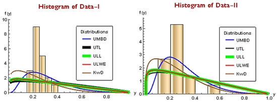
Figure 5. Histogram of competing models for Dataset I and II.

6.2.3. Dataset III

Sulfate particles are particles that contain sulfur. These are found in air particles that are smaller than one micron. They can be released from natural and manmade sources, such as industrial processes, coal burning, cement production, vehicle emissions, and sea salt [38,39,40]. Exposure to this pollutant has been associated with numerous health problems, including reduced lung function, more frequent respiratory symptoms and illnesses (like childhood bronchitis and cough), and even premature death [41]. Therefore, understanding the concentration of sulfate particles indoors or outdoors is vital for assessing their impact on air quality. In this regard, the third dataset measures the concentration of sulphate in Calgary from 31 different periods during 1995. Measurements are taken from [34] and are listed as 0.048, 0.013, 0.040, 0.082, 0.073, 0.732, 0.302, 0.728, 0.305, 0.322, 0.045, 0.261, 0.192, 0.357, 0.022, 0.143, 0.208, 0.104, 0.330, 0.453, 0.135, 0.114, 0.049, 0.011, 0.008, 0.037, 0.034, 0.015, 0.028, 0.069, and 0.029.

The analysis of the third dataset indicates that the data portray skewed and leptokurtic natures, which is displayed in Table 12. Moreover, Table 13 illustrates that the proposed model also acts as a good alternate for the competing models. Furthermore, such competence seems to emerge as strong candidate when the information criterion yields a least value, which is portrayed in Table 14.

Table 12. Descriptive statistics of Dataset III.

Size	Mean	Median	Standard Deviation	Skewness	Kurtosis	$\frac{\mathbf{S}\mathbf{k}.}{\mathbf{K}\mathbf{u}.}$
31	0.1706	0.0820	0.1944	1.6184	5.0882	0.3181

Table 13. GoF statistics of Dataset III.

Distribution	$\widehat{\mathit{\theta }}$	$\widehat{\mathit{\lambda }}$	${\mathbf{A}}^{\ast }$	${\mathbf{W}}_{\ast }$	KS	p-Value
UMBD	1.5820	------	1.3459	0.1473	0.1606	0.4001
UTL	0.5424	------	1.4801	0.2665	0.1580	0.4211
ULL	0.000001	0.8192	0.8557	0.1412	0.1261	0.7086
ULWE	0.00003	0.8192	0.8557	0.1411	0.1260	0.7086
UKw	0.7388	2.9782	0.6398	0.0956	0.1315	0.6573

Table 14. Information criterion measure of Dataset III.

Distribution	$-\mathit{l}$	$\mathbf{A}\mathbf{I}\mathbf{C}$	$\mathbf{A}\mathbf{I}\mathbf{C}\mathbf{C}$	$\mathbf{B}\mathbf{I}\mathbf{C}$	HQIC
UMBD	23.3506	−44.7012	−44.5633	−43.2672	−44.2338
UTL	21.6018	−41.2036	−41.0657	−39.7696	−40.7362
ULL	23.2327	−42.4654	−42.0368	−39.5974	−41.5305
ULWE	23.2327	−42.4654	−42.0368	−39.5974	−41.5305
UKw	23.6241	−43.2482	−42.8196	−40.3802	−42.3133

6.2.4. Dataset IV

The fourth dataset measured the concentration of pollutant CO in Alberta, Canada from the Calgary northwest (residential) monitoring unit (CRMU) station during 1995. Measurements are listed in [34] for the period 1976-95 as 0.16, 0.19, 0.24, 0.25, 0.30, 0.41, 0.40, 0.33, 0.23, 0.27, 0.30, 0.32, 0.26, 0.25, 0.22, 0.22, 0.18, 0.18, 0.20, and 0.23.

From Table 15, it is evident that dataset IV depicts positive skewness and leptokurtic behavior. However, GoF statistics as portrayed in Table 16 are least when compared with the competing models. As stated by Table 17, the information criteria of the proposed model are also yield minimum values, thus the proposed model acts as the least loss of information with single parameter.

Table 15. Descriptive statistics of Dataset IV.

Size	Mean	Median	Standard Deviation	Skewness	Kurtosis	$\frac{\mathbf{S}\mathbf{k}.}{\mathbf{K}\mathbf{u}.}$
20	0.2570	0.2450	0.0692	0.7948	2.9508	0.2694

Table 16. GoF statistics of Dataset IV.

Distribution	$\widehat{\mathit{\theta }}$	$\widehat{\mathit{\lambda }}$	${\mathbf{A}}^{\ast }$	${\mathbf{W}}_{\ast }$	KS	p-Value
UMBD	0.8161	------	1.7337	0.2975	0.2675	0.2563
UTL	1.1959	------	3.6486	0.7195	0.4005	0.0163
ULL	2.2250	7.04$\times {10}^{-33}$	3.2294	0.6113	0.3668	0.0353
ULWE	1.4378	2.89$\times {10}^{-8}$	3.2294	0.6113	0.3668	0.0353
UKw	1.2312	4.6236	3.1513	0.6289	0.4064	0.0141

Table 17. Information criterion of Dataset IV.

Distribution	$-\mathit{l}$	$\mathbf{A}\mathbf{I}\mathbf{C}$	$\mathbf{A}\mathbf{I}\mathbf{C}\mathbf{C}$	$\mathbf{B}\mathbf{I}\mathbf{C}$	HQIC
UMBD	17.9885	−33.9770	−33.7548	−32.9813	−33.7826
UTL	8.1365	−14.2730	−14.0508	−13.2773	−14.0786
ULL	8.5914	−13.1828	−12.4769	−11.1913	−12.7940
ULWE	8.5914	−13.1828	−12.4769	−11.1913	−12.7940
UKw	12.7916	−21.5832	−20.8773	−19.5917	−21.1944

Moreover, from Figure 6, it is evident that the proposed model yields good fit with the least loss of information criterion.

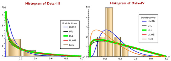
Figure 6. Histogram of competing models for Dataset-III and IV.

7. Conclusions

In this study, we have introduced a flexible single-parameter unit distribution called UMBD for modeling datasets bounded to the interval (0, 1). We have investigated the moments of the distribution and related distribution measurements, such as variance, skewness, and kurtosis. We have obtained the survival function, hrf, and rhrf of the UMBD and illustrated their behaviors through graphs. Moreover, we have obtained the moment generating and mode of the UMBD in this paper. We have investigated the inference problem for the parameter of the UMBD from the perspectives of maximum likelihood, least squares, weighted least squares, method of moments, and maximum product space methodologies. We have also performed various simulation studies to determine the estimation performances and empirical behaviors of the obtained estimators. Additionally, we have presented analyses performed on four practical datasets to demonstrate data modeling with the UMBD. We believe that the UMBD will be beneficial to data modelers and researchers from different fields and that the work in the paper will inspire the derivation of other unit distributions.

The results we obtained indicate that the UMBD would not be appropriate for modeling lifetime data with decreasing-increasing-decreasing (modified bathtub) and unimodal hazard rates shapes. As a result, these shortcomings can be fixed in a subsequent study. Additional estimation techniques, such as those based on the Bayesian perspective, may also be put forth. Furthermore, we also suggest adding a shape parameter to this model and looking into the existence of its information matrix.

References

- Mo, J.; Zhang, Y.; Xu, Q.; Lamson, J.J.; Zhao, R. Photocatalytic purification of volatile organic compounds in indoor air: A literature review. Atmos. Environ. 2009, 43, 2229–2246. [Google Scholar] [CrossRef]
- Bayes, T. An Essay Towards Solving a Problem in the Doctrine of Chances. By the late Rev. Mr. Bayes, F.R.S. communicated by Mr. Price, in a letter to John Canton, A.M.F.R. SPhil. Trans. R. Soc. 1763, 53, 370–418. [Google Scholar] [CrossRef]
- Leipnik, R.B. Distribution of the Serial Correlation Coefficient in a Circularly Correlated Universe. Ann. Math. Stat. 1947, 18, 80–87. [Google Scholar] [CrossRef]
- Johnson, N. Systems of Frequency Curves Derived From the First Law of Laplace. Trab. Estad. 1955, 5, 283–291. [Google Scholar] [CrossRef]
- Jørgensen, B. Proper Dispersion Models. Braz. J. Probab. Stat. 1997, 11, 89–128. [Google Scholar]
- Kumaraswamy, P. A generalized probability density function for double-bounded random processes. J. Hydrol. 1980, 46, 79–88. [Google Scholar] [CrossRef]
- Topp, C.W.; Leone, F.C.A. Family of J-Shaped Frequency Functions. J. Am. Stat. Assoc. 1955, 50, 209–219. [Google Scholar] [CrossRef]
- Consul, P.C.; Jain, G.C. On the Log-Gamma Distribution and Its Properties. Stat. Hefte 1971, 12, 100–106. [Google Scholar] [CrossRef]
- Concha-Aracena, M.S.; Barrios-Blanco, L.; Elal-Olivero, D.; Ferreira da Silva, P.H.; Nascimento, D.C.D. Extending Normality: A Case of Unit Distribution Generated from the Moments of the Standard Normal Distribution. Axioms 2022, 11, 666. [Google Scholar] [CrossRef]
- Dombi, J.; Jónás, T.; Tóth, Z.E. The Epsilon Probability Distribution and its Application in Reliability Theory. Acta Polytech. Hung. 2018, 15, 197–216. [Google Scholar]
- Smithson, M.; Shou, Y. CDF-Quantile Distributions for Modelling RVs on the Unit Interval. Br. J. Math. Stat. Psych. 2017, 70, 412–438. [Google Scholar] [CrossRef] [PubMed]
- Altun, E.; Hamedani, G. The Log-Xgamma Distribution With Inference and Application. J. Société Française Stat. 2018, 159, 40–55. [Google Scholar]
- Nakamura, L.R.; Cerqueira, P.H.R.; Ramires, T.G.; Pescim, R.R.; Rigby, R.A.; Stasinopoulos, D.M. A New Continuous Distribution on the Unit Interval Applied to Modelling the Points Ratio of Football Teams. J. Appl. Stat. 2019, 46, 416–431. [Google Scholar] [CrossRef]
- Ghitany, M.E.; Mazucheli, J.; Menezes, A.F.B.; Alqallaf, F. The Unit-Inverse Gaussian Distribution: A New Alternative to Two-Parameter Distributions on the Unit Interval. Commun. Stat.-Theory Methods 2019, 48, 3423–3438. [Google Scholar] [CrossRef]
- Mazucheli, J.; Menezes, A.F.; Dey, S. Unit-Gompertz Distribution with Applications. Statistica 2019, 79, 25–43. [Google Scholar] [CrossRef]
- Mazucheli, J.; Menezes, A.F.B.; Chakraborty, S. On the One Parameter Unit-Lindley Distribution and Its Associated Regression Model for Proportion Data. J. Appl. Stat. 2019, 46, 700–714. [Google Scholar] [CrossRef]
- Mazucheli, J.; Menezes, A.F.B.; Fernandes, L.B.; de Oliveira, R.P.; Ghitany, M.E. The Unit-Weibull Distribution as an Alternative to the Kumaraswamy Distribution for the Modeling of Quantiles Conditional on Covariates. J. Appl. Stat. 2019, 47, 954–974. [Google Scholar] [CrossRef] [PubMed]
- Gündüz, S.; Mustafa, Ç.; Korkmaz, M.C. A New Unit Distribution Based on the Unbounded Johnson Distribution Rule: The Unit Johnson SU Distribution. Pak. J. Stat. Oper. Res. 2020, 16, 471–490. [Google Scholar] [CrossRef]
- Altun, E. The log-weighted exponential regression model: Alternative to the beta regression model. Commun. Stat.-Theory Methods 2021, 50, 2306–2321. [Google Scholar] [CrossRef]
- Biswas, A.; Chakraborty, S. A new method for constructing continuous distributions on the unit interval. arXiv 2021, arXiv:2101.04661. [Google Scholar]
- Afify, A.Z.; Nassar, M.; Kumar, D.; Cordeiro, G.M. A New Unit Distribution: Properties and Applications. Electron. J. Appl. Stat. 2022, 15, 460–484. [Google Scholar]
- Korkmaz, M.Ç.; Korkmaz, Z.S. The Unit Log–log Distribution: A New Unit Distribution With Alternative Quantile Regression Modeling and Educational Measurements Applications. J. Appl. Stat. 2023, 50, 889–908. [Google Scholar] [CrossRef] [PubMed]
- Fayomi, A.; Hassan, A.S.; Baaqeel, H.; Almetwally, E.M. Bayesian Inference and Data Analysis of the Unit–Power Burr X Distribution. Axioms 2023, 12, 297. [Google Scholar] [CrossRef]
- Krishna, A.; Maya, R.; Chesneau, C.; Irshad, M.R. The Unit Teissier Distribution and Its Applications. Math. Comput. Appl. 2023, 27, 12. [Google Scholar] [CrossRef]
- Bakouch, H.S.; Hussain, T.; Tošić, M.; Stojanović, V.S.; Qarmalah, N. Unit Exponential Probability Distribution: Characterization and Applications in Environmental and Engineering Data Modeling. Mathematics 2023, 11, 4207. [Google Scholar] [CrossRef]
- Abramowitz, M.; Stegun, I.A. (Eds.) Handbook of Mathematical Functions with Formulas, Graphs, and Mathematical Tables; US Government Printing Office: Washington, DC, USA, 1948; Volume 55.
- Günay, F.; Yilmaz, M. Different Parameter Estimation Methods for Exponential Geometric Distribution and Its Applications in Lifetime Data Analysis. Biostat. Biom. 2018, 8, 1–8. [Google Scholar] [CrossRef][Green Version]
- Eaton, J.W.; Bateman, D.; Hauberg, S. GNU Octave Version 3.0. 1 Manual: A High-Level Interactive Language for Numerical Computations; SoHo Books: New York, NY, USA, 2007. [Google Scholar]
- Guarnieri, M.; Balmes, J.R. Outdoor air pollution and asthma. Lancet 2014, 383, 1581–1592. [Google Scholar] [CrossRef]
- Manisalidis, I.; Stavropoulou, E.; Stavropoulos, A.; Bezirtzoglou, E. Environmental and health impacts of air pollution: A review. Front. Public Health 2020, 8, 505570. [Google Scholar] [CrossRef]
- Wei, W.; Wang, Z. Impact of industrial air pollution on agricultural production. Atmosphere 2021, 12, 639. [Google Scholar] [CrossRef]
- Sangsanit, Y.; Bodhisuwan, W. The Topp-Leone generator of distributions: Properties and inferences. Songklanakarin J. Sci. Technol. 2016, 38, 537–548. [Google Scholar]
- Gómez-Déniz, E.; Sordo, M.A.; Calderín-Ojeda, E. The Log–Lindley distribution as an alternative to the beta regression model with applications in insurance. Insur. Math. Econ. 2014, 54, 49–57. [Google Scholar] [CrossRef]
- Myrick, R.H. Air Quality Monitoring in Alberta DATA REPORT 1995. Oxbridge Place: Edmonton, AB, Canada, 1996. [Google Scholar]
- Kumari, B.; Chandra, R. A Review on Bacterial Degradation of Benzo[a]pyrene and Its Impact on Environmental Health. J. Exp. Biol. Agric. Sci. 2022, 10, 1253–1265. [Google Scholar] [CrossRef]
- Slezakova, K.; Castro, D.; Pereira, M.C.; Morais, S.; Delerue-Matos, C.; Alvim-Ferraz, M.C. Influence of traffic emissions on the carcinogenic polycyclic aromatic hydrocarbons in outdoor breathable particles. J. Air Waste Manag. Assoc. 2010, 60, 393–401. [Google Scholar] [CrossRef] [PubMed]
- Iskander, K.; Gaikwad, A.; Paquet, M.; Long, D.J.; Brayton, C.; Barrios, R.; Jaiswal, A.K. Lower induction of p53 and decreased apoptosis in NQO1-null mice lead to increased sensitivity to chemical-induced skin carcinogenesis. Cancer Res. 2005, 65, 2054–2058. [Google Scholar] [CrossRef]
- Ebert, M.; Müller-Ebert, D.; Benker, N.; Weinbruch, S. Source apportionment of aerosol particles near a steel plant by electron microscopy. J. Environ. Monit. 2012, 14, 3257–3266. [Google Scholar] [CrossRef] [PubMed]
- Lin, Y.C.; Yu, M.; Xie, F.; Zhang, Y. Anthropogenic emission sources of sulfate aerosols in Hangzhou, East China: Insights from isotope techniques with consideration of fractionation effects between gas-to-particle transformations. Environ. Sci. Technol. 2022, 56, 3905–3914. [Google Scholar] [CrossRef] [PubMed]
- Ghahreman, R.; Norman, A.L.; Abbatt, J.P.; Levasseur, M.; Thomas, J.L. Biogenic, anthropogenic and sea salt sulfate size-segregated aerosols in the Arctic summer. Atmos. Chem. Phys. 2016, 16, 5191–5202. [Google Scholar] [CrossRef]
- Awopetu, M.S.; Aribisala, J.O. Air Quality Index As A Tool For Monitoring Environmental Degradation And Health Implications. Wit Trans. Ecol. Environ. 2019, 236, 9–19. [Google Scholar]
Disclaimer/Publisher’s Note: The statements, opinions and data contained in all publications are solely those of the individual author(s) and contributor(s) and not of MDPI and/or the editor(s). MDPI and/or the editor(s) disclaim responsibility for any injury to people or property resulting from any ideas, methods, instructions or products referred to in the content. |
© 2024 by the authors. Licensee MDPI, Basel, Switzerland. This article is an open access article distributed under the terms and conditions of the Creative Commons Attribution (CC BY) license (https://creativecommons.org/licenses/by/4.0/).