Article

Moduli of Continuity in Metric Models and Extension of Livability Indices

by
Roger Arnau
,
Jose M. Calabuig
,
Álvaro González
and
Enrique A. Sánchez Pérez
*
Instituto Universitario de Matemática Pura y Aplicada, Universitat Politècnica de València, Camino de Vera s/n, 46022 Valencia, Spain
*
Author to whom correspondence should be addressed.
Axioms 2024, 13(3), 192; https://doi.org/10.3390/axioms13030192
Submission received: 20 February 2024 / Revised: 11 March 2024 / Accepted: 12 March 2024 / Published: 14 March 2024

Abstract

:
Index spaces serve as valuable metric models for studying properties relevant to various applications, such as social science or economics. These properties are represented by real Lipschitz functions that describe the degree of association with each element within the underlying metric space. After determining the index value within a given sample subset, the classic McShane and Whitney formulas allow a Lipschitz regression procedure to be performed to extend the index values over the entire metric space. To improve the adaptability of the metric model to specific scenarios, this paper introduces the concept of a composition metric, which involves composing a metric with an increasing, positive and subadditive function ϕ . The results presented here extend well-established results for Lipschitz indices on metric spaces to composition metrics. In addition, we establish the corresponding approximation properties that facilitate the use of this functional structure. To illustrate the power and simplicity of this mathematical framework, we provide a concrete application involving the modeling of livability indices in North American cities.
MSC:
62J02; 26A16; 54E35

1. Introduction

Metric models, constructed from the aggregation of various variables, serve as useful frameworks that enable prospective approaches in fields such as the social sciences. One version of these models is given by so-called index spaces (see [1] and the related literature), which consist of a triple ( M , d , I ) , where ( M , d ) represents a metric space and I denotes an index (essentially, a non-negative Lipschitz function satisfying additional regularity properties). Such models prove advantageous in practical contexts, as they allow the extension of significant indices defined within a metric subspace of ( M , d ) to the entire space with the same Lipschitz norm, as seen in the classical scenario of the Lipschitz regression. This methodology is justified when attempting to model special circumstances that do not conform to linear constraints. The usefulness of these results has been demonstrated in recent years by a large number of research papers in various disciplines. For example, concrete applications can be observed in machine learning, where this conceptual framework is employed [2]. Analogous concepts are also widely used in other scientific fields [3,4].
However, there are many cases in which the metric of the problem is not established and has to be defined at some stage in the modeling process. This choice can be critical, as different metrics can lead to very different results. This article attempts to redefine this methodology by introducing a novel approach to obtain, in a straightforward manner, from a simple metric, another metric that better fits the problem. This newly proposed metric, denoted d ϕ , is chosen from the set of composition metrics ϕ d , where d is the original metric and ϕ is a continuity modulus. In particular, we show that this adaptation of the initial metric space yields significant improvements over using the original metric structure ( M , d ) . To this end, we provide an example that consists of extending the AARP livability index, known for certain US cities, to a wider range of cities, thereby evaluating and analyzing the errors incurred under different considerations. Furthermore, we introduce a new category of indices, called standard indices, aimed at increasing the effectiveness of the proposed approximation technique. In all of these cases, the Lipschitz constant, together with other normalization properties related to the Katetov condition, serves as a central tool for controlling the resulting extension over all scenarios.
The ideas presented here are not new. The notion of modulus of continuity can be found in many works, usually in the context of mathematical analysis (see [5] and the references therein). However, it is not easy to find applied works in the literature that use this tool, which is essentially of a theoretical nature. The concept of composition metrics can be found, under various names, in several works, including some articles from the early part of the twentieth century. The notion of continuous metric transformations (metric-preserving functions in the literature) is first introduced in Wilson’s 1935 article [6]. A paper by Borsík and Doboš in 1981 [5] compiles some of the conditions under which a given function composed with a metric will return a metric, and vice versa. Furthermore, the article by Valentine [7] already introduces a continuity modulus in the Lipschitz condition.
Therefore, our interest is to carry out all of this study in the framework of metric models related to the extension of Lipschitz functions, specifically by introducing a class of Lipschitz maps that aims to give a broader definition by incorporating an alternative metric for improved extension capabilities. This involves a more skillful adaptation to the dataset and an improved extension of the indices. Our research will explore the instances of this new space that are relevant to us. We will explore its relevance to the field of interest, in particular to the index theory, while analyzing its effectiveness and contrasting it with established methods. To achieve this, we have organized this paper as follows. In Section 2, we will present the main concepts on real Lipschitz functions and metric spaces and re-introduce the generalization proposal (composition metrics and other mathematical tools). Section 3 deals with the formal context of what we call indices. We will analyze spaces whose elements are these objects, exposing two methods of extension to larger domains, whose results, in practical contexts, will also be presented at the end of the paper. Thus, finally, in Section 4, we will explore the practical application of the above findings to algorithms that numerically execute the described extension procedures. We will delve into specific examples in which we examine their functionality, paying particular attention to performance differences compared to the original alternative and other potential procedures.

2. Basic Definitions and Concepts

Let us first explain some elementary facts on metric spaces and Lipschitz functions (see [8,9]). Consider a set D that is non-empty and a real map from d : D × D ( R + being the positive reals). It is said that d is a metric (distance) in the case that d ( a , b ) = 0 if a = b , symmetric (that is, d ( a , b ) = d ( b , a ) ) and transitive ( d ( a , b ) d ( a , c ) + d ( c , b ) ) for a , b , c D . The metric d is bounded if d ( x , y ) < K for a constant K. A metric subspace of D is any subset D 0 endowed with the same distance. A metric space as above is compact. For each sequence { s n } n D , there is a subsequence { s n k } k that tends to some element a D . This property is sometimes called the sequential characterization of compactness in metric spaces.
The maps we are interested in in this paper are those that satisfy the Lipschitz condition. A metric space valued function f from a metric space ( D , d ) to another metric space ( R , r ) is Lipschitz if there is a number K R that satisfies:
r ( f ( x ) , f ( y ) ) K d ( x , y ) , x , y D .
The best constant K above is what is call the Lipschitz norm (or constant), and sometimes it is said that f is K-Lipschitz. The symbol L i p ( f ) is used for the Lipschitz norm of f . Clearly,
sup x , y D , x y r ( f ( x ) , f ( y ) ) · ( d ( x , y ) ) 1 = L i p ( f ) .
Suppose f is a real function defined on D but known only in S D . Several classical results concern the extension of f to D while preserving some initial properties of f in S. The main result in this direction is when the property we want to preserve is the Lipschitz condition and is called the McShane–Whitney theorem [10,11]. Because of the useful extension formulas that can be obtained, this result has been the starting point for much research on the subject.
Theorem 1.
Let L > 0 , and let f : S D R be an L-Lipschitz map. Then, there is always an extension of f preserving the Lipschitz constant L , that is, a function F : D R satisfying F S = f . This extension can be given by any of the following formulas (sometimes called the Whitney and McShane extensions),
F W ( x ) = inf y S f ( y ) + L d ( x , y ) , F M ( x ) = sup y S f ( y ) L d ( x , y )
for every x D .
These extensions are in a sense optimal: if F is any other Lipschitz extension, we have F M F F W . Note also that F : = t F W + ( 1 t ) F M is a Lipschitz extension if t ( 0 , 1 ) , and the Lipschitz norm is also L .
The explanation and proofs of the general results on Lipschitz maps can be found in [9].

Composition Metrics and Modulus of Continuity

We now focus on the possibility of generalizing the Lipschitz condition to include a broader class of functions, satisfying a more relaxed criterion and thereby preserving the extension theorems. This paper will address this in a positive way with what we call ϕ -Lipschitz maps. First, we will define the family of maps Φ , which will serve as a form of the generalized continuity module [12]. However, our main focus will be on metrics that can be formulated as compositions of a pre-existing metric with these functions, rather than on the functions themselves. Our specific interpretation of such a continuity module is outlined below:
Definition 1.
A map ϕ : R + R + belongs to Φ when, for every x , y R + , we have:
(i). 
ϕ ( x + y ) ϕ ( x ) + ϕ ( y ) and ϕ ( 0 ) = 0 .
(ii). 
ϕ ( x ) < ϕ ( y ) when x < y .
(iii). 
ϕ is a continuous function.
As we said, such functions are often called moduli of continuity. Examples of functions belonging to Φ are ϕ ( x ) = x α for 0 < α < 1 or the sigmoid function σ ( x ) = 1 1 + e x . Thus, a modulus of continuity is defined to be an increasing function ω : [ 0 , + ) [ 0 , + ) which satisfies that ω ( 0 ) = 0 is continuous at 0. Sometimes, other requirements are imposed. For example, in [9], (Chapter 6, Section 4) continuity modules are related to metrics in a similar way to the one we present here, although restricted to the context of the study of uniform continuity.
Now, following the scheme of the definition of the Lipschitz map, we will introduce a function ϕ Φ of the distance. The definition is as follows.
Definition 2.
If ( D , d ) and ( R , r ) are metric spaces, take a map f : D R . Suppose that ϕ Φ . Then, f is a ϕ-Lipschitz map whenever we have the existence of a constant K > 0 that satisfies that, for all x , y D ,
r ( f ( x ) , f ( y ) ) K ϕ ( d ( x , y ) ) .
As in the standard case, the constant K > 0 is a Lipschitz constant of the ϕ —Lipschitz map f. We will consider a new function ϕ d = d ϕ as the composition of the distance d with ϕ Φ .
We observe that every L-Lipschitz map is also a ϕ -Lipschitz map for ϕ ( x ) = x and K = L . In addition, consider the function f : R + R + , defined as f ( x ) = x . While this function is not Lipschitz, it meets the criteria of being ϕ -Lipschitz for ϕ = f Φ and K = 1 . Thus, this category of mappings effectively generalizes the notion of the L-Lipschitz map. We will see further improvements motivated by this construction in Section 3 by means of a different map, f ( x ) = log ( x + 1 ) , for example.
We propose redefining the distance to encompass new maps satisfying the proposed condition alongside the Lipschitz maps within the resulting metric space. By adjusting ϕ , we gain direct control over modifying the original metric to better suit the posed problem. Subsequently, we will demonstrate that d ϕ indeed constitutes a valid distance.
Proposition 1.
If ( D , d ) is a metric space, and supposing that ϕ Φ , then we have that d ϕ is a distance too.
Proof. 
Because ϕ is an injective function (due to its strict monotonicity) and ϕ ( 0 ) = 0 , it is evident that d ϕ ( x , y ) = 0 if and only if d ( x , y ) = 0 . Since d is a metric, this occurs if and only if x = y , establishing the identity of indiscernibles for d ϕ . The symmetry of d implies directly the symmetry of d ϕ . Considering the triangle inequality, monotonicity and subadditivity of ϕ, we have
d ϕ ( x , z ) ϕ ( d ( x , y ) + d ( y , x ) ) d ϕ ( x , y ) + d ϕ ( y , z ) .
Consequently, d ϕ is a distance. □
The reciprocal of this result is usually false. For example, if D = R and we let ϕ Φ be ϕ ( x ) = x for x 0 , and d ( x , y ) = | x y | 2 , we know that d ϕ = | x y | is a metric on D, while d is not. To illustrate this, consider taking x = 0 , y = 1 and z = 3 , and observe that d ( x , z ) > d ( x , y ) + d ( y , z ) , which violates the triangle inequality. However, there exists a sort of converse implication. Assuming that for any metric space ( D , d ) , the function d ϕ constitutes a metric, we can infer certain conditions that ϕ must meet. For instance, it is straightforward to verify that ϕ ( 0 ) = 0 . Moreover, we will demonstrate next that ϕ must exhibit subadditivity.
Let x , y R + and define a metric space D = { a , b , c } such that d ( a , b ) = x , d ( b , c ) = y and d ( a , c ) = x + y . Such a d is evidently a metric on D. Since d ϕ is a metric, applying the triangle inequality yields ϕ ( x + y ) = d ϕ ( a , c ) d ϕ ( a , b ) + d ϕ ( b , c ) = ϕ ( x ) + ϕ ( y ) , thus establishing the subadditivity of ϕ . Thus, if a function ϕ : R + R + satisfies that d ϕ is a metric for all metrics d , then ϕ is subadditive and ϕ ( 0 ) = 0 . However, there might be instances where the required conditions of monotonicity and continuity for ϕ are not fulfilled. In other words, d ϕ can qualify as a metric for every metric space ( D , d ) without ϕ being strictly monotonically increasing or continuous. For instance, consider ϕ defined as follows: ϕ ( x ) = 0 if x = 0 , and ϕ ( x ) = 1 if x > 0 . For each metric space ( D , d ) , we observe the following:
(a)
For any a , b D , the condition d ϕ ( a , b ) = 0 holds if and only if d ( a , b ) = 0 because ϕ is only null at 0. Since d is a metric, this holds if and only if a = b , demonstrating that d ϕ satisfies the identity of indiscernibles.
(b)
Given that d ( a , b ) = d ( b , a ) for all a , b D , it is evident that d ϕ ( a , b ) = d ϕ ( b , a ) , indicating the symmetry of d ϕ .
(c)
Let a , b , c D with corresponding distances x = d ( a , b ) , y = d ( b , c ) and z = d ( a , c ) . If a , b , c are distinct, then x , y , z > 0 since d is a metric, leading to ϕ ( x ) = ϕ ( y ) = ϕ ( z ) = 1 .
Consequently, d ϕ satisfies the triangle inequality for a , b , c . In cases where some elements of D coincide, the triangular inequality for d ϕ trivially holds for them.
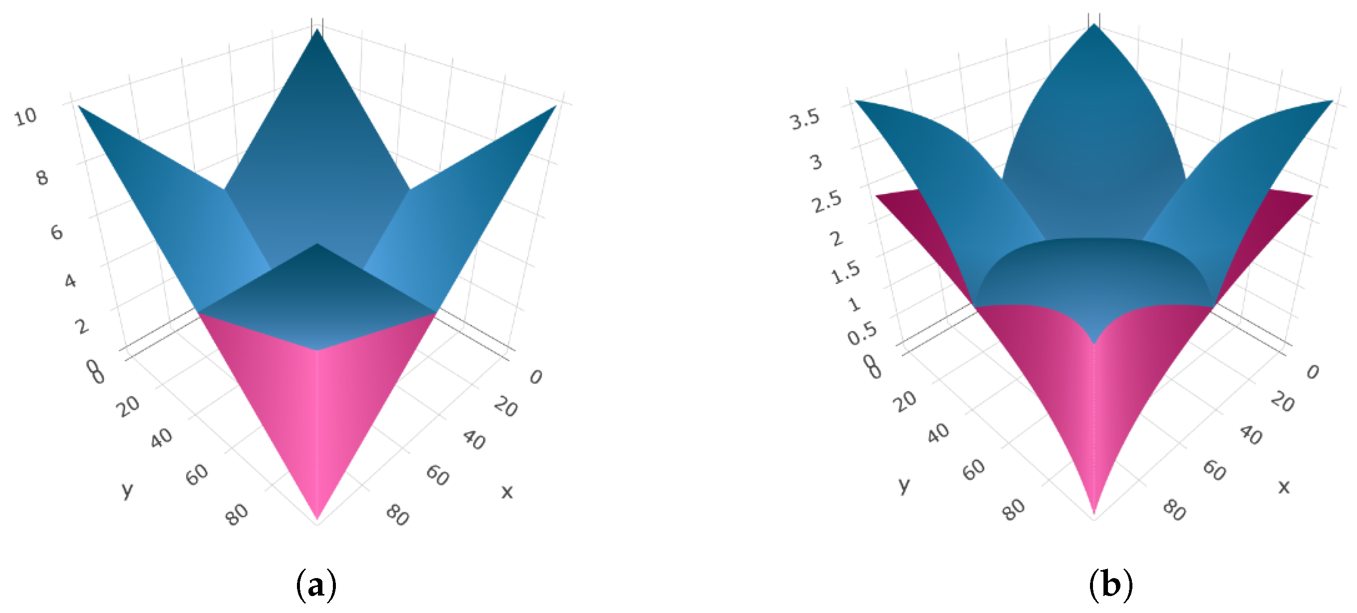
To better comprehend the relationship between d and d ϕ , we depict in Figure 1 and Figure 2 a visual representation of the behavior of two specific metrics: the Euclidean metric d in R and its composition with ϕ ( x ) = log ( 1 + x ) , denoted as d ϕ . In Figure 1, it is evident that d ϕ “smoothens” the distance between two real numbers concerning d. More precisely, d and d ϕ exhibit similar behavior when x and y are “close” to each other, but, for more distant values, d ϕ dampens the growth in comparison to d. Figure 2 offers a comparison of the triangular inequality behavior between d and d ϕ . Once again, we observe how the logarithmic growth of ϕ influences d ϕ and its triangular inequality,
d ϕ ( x , y ) , ( z , t ) = log 1 + ( x z ) 2 + ( y t ) 2 .
Example 1.
Additional examples of ϕ-Lipschitz maps are provided below:
  • A mapping f : R n R is termed α-Hölder continuous if there exist constants C > 0 and α > 0 satisfying for all x , y D
    r ( f ( x ) , f ( y ) ) C d ( x , y ) α .
    These mappings qualify as ϕ-Lipschitz maps for K = C . Specifically, if α ( 0 , 1 ] , then defining ϕ ( x ) = x α places ϕ within Φ, and f is ϕ-Lipschitz with K = C . If α > 1 , it can be demonstrated that f becomes a constant map, rendering it ϕ-Lipschitz for any α 0 .
  • Consider R equipped with its standard metric, and let ϕ Φ . Subadditivity implies ϕ ( x ) ϕ ( y ) ϕ ( x y ) for x y ; hence, d ( ϕ ( x ) , ϕ ( y ) ) ϕ ( d ( x , y ) ) . Thus, every ϕ Φ qualifies as a ϕ-Lipschitz function with K = 1 . Examples of ϕ functions, in addition to those already mentioned, include ϕ ( x ) = arctan ( x ) , ϕ ( x ) = x ( x + 1 ) 1 or ϕ ( x ) = x ( x 2 + 1 ) 1 / 2 .
The compactness for subsets of the metric spaces ( D , d ϕ ) in terms of the compactness of ( D , d ) is straightforward. For example, in ( R 2 , d ϕ ) with d ϕ , as in (1), any closed ball is compact.
Proposition 2.
Suppose that ( D , d ) is compact. Then, for every function, ϕ Φ   ( D , d ϕ ) is also compact.

3. Index Extension

The aim of this section is to adapt the concepts of index and index space in the terms that were introduced in [1] to the context of the composition metrics. We will also explain the extension methods available to obtain an approximation framework for Lipschitz regression. The first is supported by what are known in [1] as standard indices, which are essentially defined by the distance to a reference point. The second one is an application of the already explained McShane and Whitney extension formulas.
Our models essentially consist of a metric space ( D , d ) and an index I (a real Lipschitz map) defined on it. These indices give meaningful values to the elements of D, which are the objects of the models. The Lipschitz condition of the index is the tool that introduces a certain concordance of the metric with the nature of the distance in D. The essence of the research we propose in this paper is that we introduce another tool to improve models based on index spaces: the construction of composition metrics d ϕ that improve the fit of the metric to the situation we want to model.
The term index space is defined in [1] as a triplet ( D , d , I ) where I : D R serves as the index function, which is considered bounded if sup a D | I ( a ) | C for some C > 0 . The infimum of all such constants C satisfying this inequality is denoted as B ( I ) , represented by B ( I ) = sup a D | I ( a ) | . When discussing the normed space structure of the space of functions with the uniform norm, we use | · | in place of B ( · ) .
We will need two more boundedness-type properties to characterize the set of indices we are interested in.
Definition 3.
Consider a function I : D R to be an index. If Q > 0 , we say that it is Q-normalized when for all a , b D
d ϕ ( a , b ) Q ( | I ( a ) | + | I ( b ) | ) .
This kind of map is sometimes called a Katetov function. The normalization constant N ( I ) for I is the optimal Q . If ϕ Φ , the index I is said to be ϕ-coherent for K > 0 if for all a , b D
| I ( a ) I ( b ) | K d ϕ ( a , b ) ,
which means that it is ϕ-Lipschitz for K. The coherence constant C ( I ) for I is the infimum of all K’s.
In practical scenarios involving the construction of models using index spaces, the index value might not be readily accessible for every element within the metric space. This situation can arise when acquiring all the necessary data for the model’s context is either costly or infeasible. Hence, it becomes advantageous to possess tools enabling the approximation of the index from non-indexed elements. As previously mentioned, this section proposes two methods to address this challenge: firstly, by identifying or approximating the desired index using what we term as standard indices, and, secondly, by approaching the question as a Lipschitz regression problem using the classical extension formulas. Both techniques can be adapted to the case of composition metrics, as we will see below.

3.1. Standard Indices and Approximation

A distance function d allows us to define indices that are inherently natural, known as standard indices. For a given point a D , we can define an index I a as I a ( b ) : = d ( a , b ) , where b D . These functions are called standard indices. Usually, the criterion for selecting a involves identifying the element that minimizes specific properties, although any other element could be chosen instead. The aim of this section is to introduce an additional tool, the composition metric d ϕ , which allows us to use the associated standard indices b d ϕ ( a , b ) . Our interest, therefore, is in showing a method for approximation by means of standard indices or any other index. We will first present some results about the compactness of these function spaces to establish the framework. We will then turn our attention to the central issue of approximation. The main goal is to show that a robust approximation method is possible, at least in theory.
Note that uniformly bounded sets of indices (without Lipschitz-type requirements) are pointwise compact. Indeed, let C > 0 and consider the set of functions F C : = { I : D R : B ( I ) C } . There are two topologies that can be defined here: the norm topology (for B ( I ) : = sup a D | I ( a ) | ) and the one of the pointwise convergence.
If a constant k satisfies | k | C , take F C , k : = { I : D R : k B ( I ) C } . It is a compact space with the topology of pointwise convergence since each element of { I η } η Λ can be seen as a member of Π a D [ k , C ] , which is a product of compact sets in a space with the topology of the product. By Tychonoff’s theorem, it is compact.
However, although we cannot expect compactness with respect to the topology of uniform convergence of the entire space of uniformly bounded functions, the space of standard indices is compact.
Proposition 3.
Let ϕ Φ . Let ( D , d ) be a compact metric space. Then there exists C > 0 such that the space S : = { d ϕ ( a , · ) : a D } of standard indices associated with the metric d ϕ , is included in F C , which is compact in the uniform topology.
Proof. 
First, note that due to the compactness of ( D , d ) , the metric d is bounded by a certain constant R > 0 . Then, S is bounded by C : = ϕ ( R ) and so S F C . In addition, let { d ϕ ( a n , · ) } n S . By the compactness of ( D , d ) again and by Proposition 2, we already know that ( D , d ϕ ) is compact, so the sequence a n n has a subsequence a n k k that converges to a 0 D with respect to d ϕ . For any ε > 0 , there exists k 0 N such that d ϕ ( a n k , a 0 ) < ε for all k k 0 . Then, for any b D , using the triangular inequality, we have for k k 0
sup b D | d ϕ ( a n k , b ) d ϕ ( a 0 , b ) | sup b D d ϕ ( a n k , a 0 ) = d ϕ ( a n k , a 0 ) < ε .
Therefore, d ϕ ( a n k , · ) k converges uniformly to d ϕ ( a 0 , · ) . □
This allows us to obtain that there is always a best approximation for each Lipschitz index I by the elements of S , as stated in Corollary 1.
Corollary 1.
Let ϕ Φ and ( D , d ) be a compact metric space. For every function I, which is a Lipschitz index acting in the compact space ( D , d ϕ ) , there is an element a 0 S such that the standard index I a 0 , ϕ is the best approximation to I in S , that is,
inf { I I a , ϕ : a D } = I I a 0 , ϕ .
Proof. 
A direct compactness argument gives the proof. The function F : S R defined as
F ( I a , ϕ ) = I I a , ϕ , a D ,
is continuous (and even Lipschitz), since
| F ( I a , ϕ ) F ( I b , ϕ ) | = | I I a , ϕ I I b , ϕ | I a , ϕ I b , ϕ
= sup c D | ϕ d ( a , c ) ϕ d ( b , c ) | ϕ d ( a , b ) = d ϕ ( a , b ) ,
for all a , b D . The compactness of S (Proposition 3) proves the result. □
Let us now focus our attention on the approximation bound for general Lipschitz indices. In particular, we will show that we can always obtain an estimate of the error made by this approximation procedure in terms of the generalization of the normalization and the coherence constants. For technical reasons, we also need to introduce a specific type of sequence that will feature the result we are seeking.
A sequence a n n D is termed pointwise Cauchy if, for each b D , the sequence lim n d ( a n , b ) exists. Every convergent sequence is pointwise Cauchy, but the converse is not necessarily true. For instance, the sequence a n = 1 / n in D = ( 0 , 1 ] with the Euclidean metric serves as an example of a non-convergent pointwise Cauchy sequence. The definition above can directly be translated for the composition metrics d ϕ , ϕ Φ .
The following result will finally give us the tool to approximate an index using the standard indices, in the sense of an improvement to [1], (Th. 1). We will also see that this approximation depends on the product of the normalization and coherence constants. Specifically, we will see these results for the following set of indices to be approximated:
R K , Q , C : = I 0 : | I ( a ) I ( b ) | K d ϕ ( a , b ) , 1 + K Q K inf ( I ) + d ϕ ( a , b ) Q ( I ( a ) + I ( b ) ) , B ( I ) C .
The proof of the following result is similar to the theorem discussed before. We include the proof for the aim of completeness.
Theorem 2.
Let K , Q > 0 such that K Q 1 . For every I R K , Q , C , there is a sequence { a n } n that is pointwise Cauchy and I ( b ) inf ( I ) + lim n K d ϕ ( a n , b ) K Q I ( b ) , b D .
Proof. 
Take b D and fix n N . Then, for every n N , there is an element a n D such that I ( a n ) 1 n inf ( I ) and so
inf ( I ) + K d ϕ ( a n , b ) K Q I ( a n ) + K Q I ( b ) K Q inf ( I ) K Q I ( b ) + K Q I ( a n ) K Q I ( a n ) 1 n = K Q I ( b ) + K Q n .
In addition,
I ( b ) I ( a n ) | I ( b ) I ( a n ) | K d ϕ ( a n , b ) ,
and therefore
I ( b ) K d ϕ ( a n , b ) + I ( a n ) K d ϕ ( a n , b ) + inf ( I ) + 1 n K Q I ( b ) + 1 + K Q n ,
for all n N and b D . Now, observe that d ϕ ( a n , · ) = I a n ( · ) S . Thus, leveraging the compactness of S, as demonstrated in Proposition 3, there exists a subsequence a n k k such that lim k d ϕ ( a n k , b ) = d ϕ ( a 0 , b ) for each b D and some a 0 D . Consequently, a n k k forms a pointwise Cauchy sequence, and, based on the last inequality, we conclude that
I ( b ) inf ( I ) + K lim k d ϕ ( a n k , b ) K Q I ( b ) , b D .
So, the function I ˜ : = inf ( I ) + K lim k d ϕ ( a n k , · ) can be seen as an approximation for I R K , Q , C . The maximum error committed is bounded by
sup b D | I ˜ ( b ) I ( b ) | sup b D | K Q I ( b ) I ( b ) | = ( K Q 1 ) C .
If K Q 1 , the comparison between I ˜ and I is reasonable. However, as these constants increase, the approximation may deteriorate.
Furthermore, by setting b = a 0 in the result of Theorem 2, we obtain
I ( a 0 ) inf ( I ) + K lim k d ϕ ( a n k , a 0 ) = inf ( I ) + K d ϕ ( a 0 , a 0 ) = inf ( I ) .
Therefore, I ( a 0 ) = inf ( I ) . Hence, we can express I ˜ ( · ) = I ( a 0 ) + d ϕ ( a 0 , · ) , where a 0 D is a point at which I attains its minimum. Additionally, for the indices we work with, we can assume inf ( I ) = 0 , allowing us to make this approximation for any Q-normalized and ϕ -coherent index for K. In this scenario, K I ˜ ( · ) = d ϕ ( a 0 , · ) .
Remark 1.
The condition Q K 1 stated in Theorem 2 is, in a way, universal in index spaces. This is because I 0 , and I reaches its minimum at b D (which occurs, for example, when D is finite or compact), and this minimum is 0. Hence,
I ( a ) = I ( a ) I ( b ) = | I ( a ) I ( b ) | K d ϕ ( a , b ) K Q ( I ( a ) + I ( b ) ) = K Q I ( a ) .
Consequently, if there is b D with I ( b ) = 0 , we also have K Q 1 . Moreover, even if such a scenario does not arise, in the case of I within a compact space, we have inf ( I ) = I ( b ) for a b D , implying that I 0 ( a ) : = I ( a ) I ( b ) constitutes a non-negative index that retains the characteristics of I, with I 0 ( b ) = 0 .

3.2. McShane and Whitney Formulas as Approximation Tools

Another approach to the extension problem is to formulate an estimate by means of the expressions for extending Lipschitz functions outlined in Section 2. While there are alternative expansion techniques, such as those discussed in [13], which may be more suitable for specific purposes, for our overarching application it proves more advantageous to use the classical McShane and Whitney formulas. The method follows the procedure explained in [1], adapted to the case of the composition metric. A full explanation can be found in Section 4 of that article and in the example given in Section 5 of the same article.
Remark 2.
To ensure that the composition d ϕ defines a metric, in the proof of Proposition 1, we only considered properties (i)–(iii) of Φ. That is, the continuity property is not necessary, although it was needed to ensure the compactness results for standard indices and to obtain the result of Theorem 2. However, this is not the case for these results on the McShane–Whitney extensions, since all that is required is that d ϕ defines a metric. Thus, the functions of Φ can be more general than a continuity modulus for this technique.
Convex combinations of the classical extension formulas can also be used. Furthermore, as in the case of standard indices, the product of the normalization and coherence constants is related to the accuracy of the approximation. Note that
I W ( a ) = inf b D { I ( b ) + K d ϕ ( a , b ) } inf b D { I ( b ) + K Q ( I ( a ) + I ( b ) ) } = ( 1 + K Q ) inf b D I ( b ) + K Q I ( a ) ,
for any a D . So,
sup a D | I W ( a ) I ( a ) | ( 1 + K Q ) | inf b D I ( b ) | + | K Q 1 | sup a D | I ( a ) | .
If we suppose that inf b D I ( b ) = 0 and K Q 1 , as in the case of standard indices, the last bound is reduced to
sup a D | I W ( a ) I ( a ) | ( K Q 1 ) C ,
what indicates that the approximation improves when K Q 1 . Similar bounds can be found for the McShane formula and then for any convex combination of both.

4. Applications: The Livability Index for Cities

In this section, we outline a methodological approach for practically implementing the theoretical concepts discussed in this paper to extend a given index. We begin with a finite set of elements characterized by certain real variables, where the value of a specific index I needs to be determined. For some of these elements, the value of the index is already known. Our objective is to extrapolate this known information to estimate the value of the index for elements where it is not yet defined. Mathematically, this set forms a metric space D, equipped with a suitable distance metric tailored to the nature of the data or the problem under consideration. Additionally, there exists a known index within a subset D 0 D that we aim to extend to the entire space D. To accomplish this objective, we propose the next procedure.

4.1. Methodology

The first matter we analyze is whether the diverse characteristics of the variables could distort the distance under consideration, given the heterogeneity of their scales. To mitigate this potential problem, we suggest normalizing the variables to a common scale by the following method: we subtract the minimum and divide by the interval in the range. That is, let D = { y j } j = 1 n and y j = ( x 1 j , , x m j ) . Let a k : = max j x k j and b k : = min j x k j for each k = 1 , , m . We then transform
x k j x k j b k a k b k ,
for all j and k, ensuring that the new variables are restricted to the interval [0,1], maintaining the same scale.
In order to evaluate the accuracy of the upcoming approximation, we require a measure of the error incurred, the Root Mean Square Error (RMSE). This metric provides the expected error that is given by
RMSE = 1 n j = 1 n I ˜ ( a j ) I ( a j ) 2 ,
where a 1 , , a n represent the observations for which we aim to estimate the error, and I ˜ denotes the approximation to I. However, given the absence of information about the index values we seek to approximate, we require a strategy to estimate this error. In our approach, we partition D 0 , the subset of observations with known indices, into two subsets: a training set and a test set. Seventy percent of the total observations are randomly selected for the training set, which we use to perform the expansion. The remaining observations from the test set are then utilized to calculate the Root Mean Square Error (RMSE). However, the inherent randomness in this process may influence the resulting error, rendering it potentially non-representative. To address this issue, we employ the method of cross-validation. This implies the repetition several times (twenty) and considers the respective errors to give a more consistent result in terms of accuracy.
In order to select a ϕ function that best fits the model, we engage in an optimization process aimed at minimizing the error bound on the test set. According to Theorem 2, this means minimizing the product of the coherence and normalization constants. We would partition our dataset into three subsets: the training and test subsets mentioned earlier, along with a validation subset used for fitting. However, due to the potentially limited number of available observations, the resulting subsets may not be sufficiently significant for this study. Therefore, we will utilize the values obtained from the test set as a reference for our optimization process. To accomplish this, we will consider that the linear combination of functions in Φ with positive scalars is another function in Φ . We will first select a set of elementary functions ( ϕ j ) j = 1 n Φ , and then examine for which values λ 1 , , λ n 0 the function ϕ : = λ 1 ϕ 1 + + λ n ϕ n ensures that the metric d ϕ is optimal in terms of the bound. For this purpose, we will employ the particle swarm optimization algorithm available in the R library “pso”. Unlike algorithms based on the gradient of the function, this type of algorithm explores the entire possible set of parameters, thereby avoiding convergence to non-absolute minima.
Taking the Whitney and McShane extensions, we may analyze whether we can consider an intermediate extension that optimizes the error. That is to say, to find the value α [ 0 , 1 ] for which the formula I : = ( 1 α ) I W + α I M makes the error to be minimum. The better way to obtain this real number would be by considering a validation set, but, as we explained above, we will use the test set instead. So, we determine the parameter α using the next result.
Proposition 4.
Let I : D 0 D R be an index that is ϕ-coherent, K > 0 . Let S 1 , S 2 D 0 such that S 1 S 2 = D 0 and S 1 S 2 = . Consider
I W ( b ) = inf { a S 1 : I ( a ) + K d ϕ ( a , b ) } , I M ( b ) = sup { a S 1 : I ( a ) K d ϕ ( a , b ) } .
Naming I α E : = ( 1 α ) I W + α I M , then
min 0 α 1 b S 2 I ( b ) I α E ( b ) 2 = b S 2 I ( b ) I α 0 E ( b ) 2 ,
for
α 0 = b S 2 I W ( b ) I ( b ) I W ( b ) I M ( b ) b S 2 I W ( b ) I M ( b ) 2 .
Proof. 
Consider F ( α ) = b S 2 I ( b ) I α E ( b ) 2 . We can see that
F ( α ) = b S 2 I ( b ) I W ( b ) + α I W ( b ) I M ( b ) 2 ,
so
F ( α ) = 2 b S 2 I ( b ) I W ( b ) + α I W ( b ) I M ( b ) I W ( b ) I M ( b ) + 2 α b S 2 I W ( b ) I M ( b ) 2 .
The solution of the equation F ( α ) = 0 gives the desired value of α 0 , taking into account that
F ( α ) = 2 b S 2 I W ( b ) I M ( b ) 2 0 .
We opted to utilize the Root Mean Square Error (RMSE) as the error metric instead of other alternatives because it ensures the differentiability of the function F under consideration. This facilitates a straightforward analysis of its minimum, as demonstrated in the previous proposition. Opting for other error measures defined in terms of absolute value, such as Mean Absolute Error (MAE) or Symmetric Mean Absolute Percentage Error (SMAPE), would necessitate a more intricate and indirect approach to determine the optimal α due to the non-differentiable nature of such definitions. If we consider extending by identifying the index with a standard one, we proceed to locate the element a 0 D that minimizes the index. In this scenario, we take I ˜ ( b ) : = K d ϕ ( a 0 , b ) to find an estimate of I ( b ) , taking into account min ( I ) = 0 after processing. However, it is also important to note that the choice of how we quantify an error can lead to different extensions. For example, RMSE is known to be sensitive to outliers, so minimizing this measure tends to result in models that are more sensitive to large errors. Conversely, favoring SMAPE minimization leads to models that take into account the proportional accuracy of predictions, making them more robust to outliers and better suited to scenarios in which relative accuracy is important. Thus, the choice ultimately depends on the specific objectives and requirements of the problem domain.

4.2. Extension of a Livability Index

In the following, we will validate our proposed approach using the so-called AARP Livability Index. In 2018, 55 percent of the world’s population lived in urban areas, a figure that is expected to rise to 68 percent by 2050, according to [14]. The rapid urbanization emphasizes the increasing significance of examining and quantifying concepts such as quality of life or livability in cities, as evidenced by various indices detailed in [15]. The objectives of these indices are twofold: firstly, to conceptualize livability and determine the parameters that characterize it and, secondly, to offer insights into which cities or neighborhoods provide superior living conditions. Equipped with this knowledge, urban planners can identify areas in need of intervention, while public administrations can target development and investment initiatives in regions with poor living conditions. However, assessing livability can be a complex task due to the large number of factors involved, many of which are difficult to assess. For example, T h e E c o n o m i s t ’s “Global Liveability Index”, one of the most widely used, includes thirty indicators across five categories, with some indicators building on others. In addition, certain factors, such as climate discomfort for travelers or levels of corruption, are subjective and inherently difficult to quantify. In this section, we propose the utilization of the index extension theory developed in the previous section to approximate livability using only indicators related to alternative mobility. The aim is to shift the focus away from subjective or complex social indicators and instead concentrate on factors that can be easily estimated based on existing infrastructure and the connectivity of urban patterns.
Let us elaborate on the datasets we will utilize. Walk Score® https://www.walkscore.com (accessed on 12 January 2024) is a website that assesses the walkability performance of 123 cities in the United States and Canada on a scale from 0 to 100. This assessment is based on various parameters such as intersection density, block length, and access to amenities within a 5 min walk. Additionally, Walk Score employs a similar scoring system to evaluate cities’ performances for walking and cycling. Our objective is to use these three indicators to approximate the AARP Livability Index https://livabilityindex.aarp.org/scoring (accessed on 11 November 2023). This index evaluates 61 different indicators across seven categories (housing, neighborhood, transportation, environment, health, engagement and opportunity) to gauge the livability of US cities, including factors such as housing costs, crime rates, air quality and income inequality. The resulting score ranges from 0 to 100, with 50 representing an average score, higher scores indicating above-average performance and vice versa.
In mathematical terms, our metric space is D [ 0 , 100 ] 3 , where each element ( x , y , z ) D represents a city with walk, transport and bike scores x , y and z, respectively, equipped with the canonical metric d of R 3 . For 101 US cities, we have defined the index of interest, which we will refer to as I, and our objective is to define it for 22 Canadian cities as well. Table 1 provides an example of our dataset.
We have implemented the extension of our index according to the considerations of Section 4.1. In particular, for illustrative purposes, we study our method by considering two linear combinations of functions of Φ as follows:
ϕ ( x ) = p 1 x + p 2 log ( 1 + x ) + p 3 arctan ( x ) + p 4 x 1 + x , p 1 , , p 4 0 ,
and
ψ ( x ) = p 1 x + p 2 log 1 + x + p 3 arctan x + p 4 x 1 + x , p 1 , , p 4 0 .
Table 2 presents a comparative analysis of the two extension procedures studied (standard indices and McShane–Whitney type approximation) and of the various metrics considered. The results show that writing our index as a standard index provides poor performance (a high mean error, making it unsuitable for consideration). As far as the McShane–Whitney-type formulas are concerned, it preserves the standard deviation, also reducing the expected RMSE a little. However, it should be noted that our technique requires a longer computation time, mainly due to the optimization process involved. This time can vary according to the optimization algorithm chosen and the dimension of the problem, although, as we will see, it can be similar to most techniques used today.
Furthermore, Table 3 provides the result when a convex expression as ψ is considered in this scenario, alongside the results of the classical technique. In particular, there is a better result when compared with the original metric, particularly noticeable in the case of standard indices. This variance in performance highlights the fact that the choice of the ϕ -metric has a significant impact on the degree of improvement obtained relative to the original metric. Another option would be to use the concept of local Lipschitz to split up our problem and obtain locally better Lipschitz constants. We could see whether it is more efficient to have many fast classical local extensions, or one global but slower one, using an approximation in the context of the ϕ -Lipschitz functions.
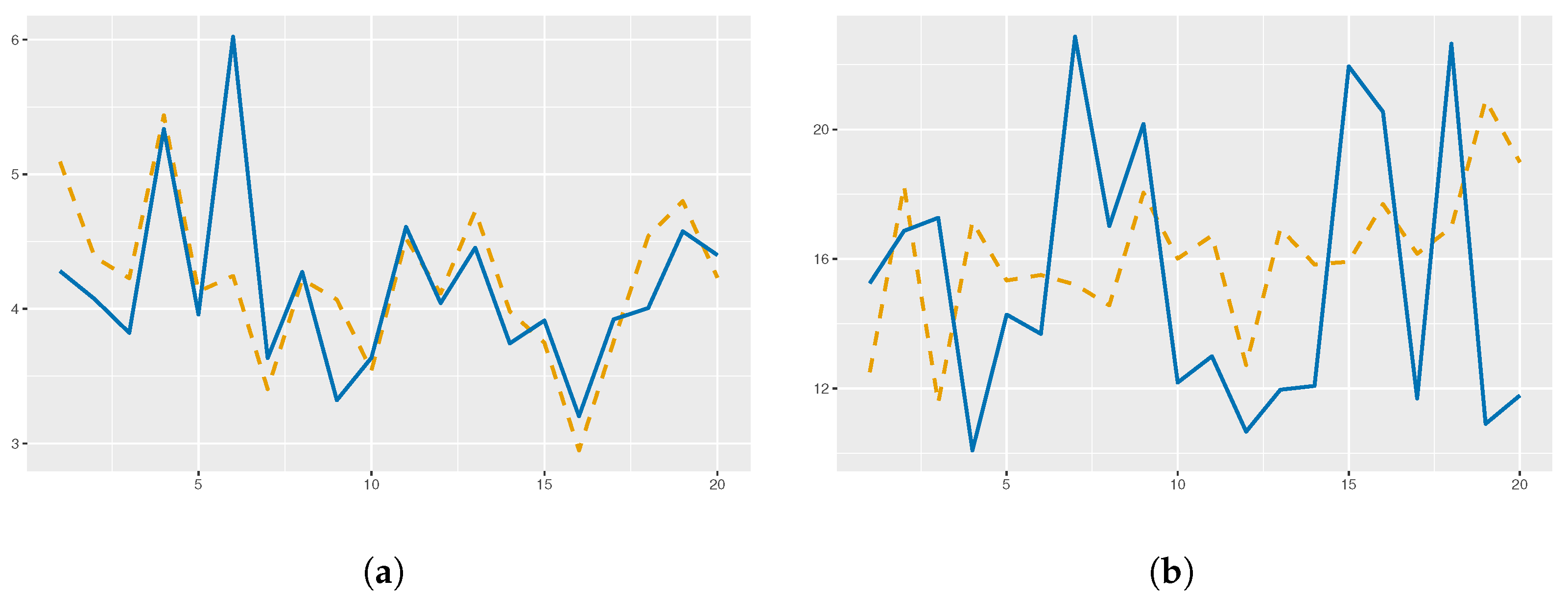
We also provide a comparison of these results with those obtained by applying different regression algorithms widely studied in the literature: neural networks and linear regression. The results of this comparison are summarized in Table 4. It is noteworthy that the results obtained by a neural network are comparable to those obtained by the McShane–Whitney technique, both in terms of the estimated error and its deviation and in terms of execution time. We can also compare the performance of the standard indices with that of a linear regression. For our example, similar results are obtained, except for the computation time, where linear regression proves to be more efficient. To allow a more comprehensive comparison of these behaviors, Figure 3 illustrates the different errors obtained in each iteration of the cross-validation. Each of the ψ metric models is plotted next to the most similar one discussed above.
It should also be noted that the way in which this improvement is achieved could vary from one method to another and from one metric to another. With this in mind, we have taken a concrete division into training and test sets (the 71 most populated cities will serve as the training and the rest as the test) and applied the results of the extension studied. In the case of standard indices, if we look at Figure 4, we can see that by redefining the metric to d ϕ or d ψ , the improvement is general, i.e., we obtain a lower error for each element following the original trend. However, in the case of the McShane–Whitney method, Figure 5 shows that depending on the new metric, the accuracy can be different for each element, although on average it is lower, as we have seen before.
Finally, in Table 5, we will present the predictions generated by each method and provide a ranking based on these predictions. Given that we lack a benchmark for our index, we will assess its performance by comparing it with other existing indices when evaluating the resulting rankings. “The Mercer Quality of Living City Ranking” https://mobilityexchange.mercer.com/Insights/quality-of-living-rankings (accessed on 3 December 2023) ranks Canadian cities in the following increasing order: Calgary, Ottawa, Toronto and Vancouver. It is noteworthy that this ranking is largely consistent with the one we have derived. Although the standard indices may not offer an exact approximation of the index in question, they still provide a reliable overview for establishing a ranking.

5. Conclusions

We have introduced an innovative procedure for the extension of indices defined on metric subspaces of metric models. The main contribution of our results is that they include a new class of metrics (composition metrics) that give us more flexibility in the approximation tools for finding adapted results of Lipschitz regression processes. While the state-of-the-art Lipschitz extensions are highly dependent on the chosen metric, this methodology provides us with a straightforward way to improve extension results without a complex study of which metrics are well suited to the problem. In particular, the introduction of this wide class of metrics starting from a standard distance (e.g., the Euclidean distance) allows this improvement by reducing the Lipschitz constant. We provide the approximation formulas as well as the error bounds for the proposed procedure. However, the limitation of reducing the use of experimental data has to be taken into account, as some variables (those involved in the definition of the metric) are necessary for the application of the model. Only a subset of the index dataset can be artificially reconstructed using the proposed method; otherwise, the reliability of the results is not guaranteed.
As an applied example, we show how we can extend the so-called livability index for large urban centers in the United States, for which this index is known, from Canadian cities. These results are interesting as they provide more information on a topic of current interest. The results show that our techniques produce similar results to other widely used techniques, with the advantage of better interpretability.
The methodology presented here can be applied to a broad class of problems where classification is performed by one or more specific indices. Lipschitz extensions can be used to obtain a combined technique for analyzing livability indices as the core of our research plan. On the one hand, we measure experimental data to obtain real information. On the other hand, this information is complemented by a new classification of cities based on the extension of the experimental data. By adding both inputs in an optimal way, in this work, we have shown that consistent results can be obtained without the need to increase the experimental work too much, making quality research on the livability of cities possible using fewer resources.

Author Contributions

Conceptualization, R.A., Á.G. and E.A.S.P.; formal analysis, R.A. and E.A.S.P.; investigation, J.M.C., Á.G. and E.A.S.P.; methodology, R.A. and Á.G.; supervision, J.M.C.; writing—original draft, Á.G. and E.A.S.P.; writing—review and editing, R.A. and J.M.C. All authors have read and agreed to the published version of the manuscript.

Funding

Enrique A. Sánchez Pérez was supported by Grant PID2020-112759GB-I00 funded by MCIN/AEI/10.13039/501100011033. Roger Arnau was supported by a contract of the Programa de Ayudas de Investigación y Desarrollo (PAID-01-21), Universitat Politècnica de València.

Institutional Review Board Statement

Not applicable.

Data Availability Statement

Figures and algorithms are available via GitHub https://github.com/Algoncor/Composition-metrics (accessed on 28 February 2024).

Conflicts of Interest

The authors declare no conflict of interest.

References

  1. Erdoğan, E.; Ferrer-Sapena, A.; Jiménez-Fernández, E.; Sánchez-Pérez, E.A. Index spaces and standard indices in metric modelling. Nonlinear Anal. Model. Control 2022, 27, 803–822. [Google Scholar] [CrossRef]
  2. Calabuig, J.; Falciani, H.; Sánchez-Pérez, E. Dreaming machine learning: Lipschitz extensions for reinforcement learning on financial markets. Neurocomputing 2020, 398, 172–184. [Google Scholar] [CrossRef]
  3. Mémoli, F.; Sapiro, G.; Thompson, P.M. Geometric surface and brain warping via geodesic minimizing Lipschitz extensions. In Proceedings of the 1st MICCAI Workshop on Mathematical Foundations of Computational Anatomy: Geometrical, Statistical and Registration Methods for Modeling Biological Shape Variability, Munich, Germany, 9 October 2006; pp. 58–67. [Google Scholar]
  4. Dacorogna, B.; Gangbo, W. Extension theorems for vector valued maps. J. Math. Pures Appl. 2006, 85, 313–344. [Google Scholar] [CrossRef]
  5. Doboš, J.B. Functions whose composition with every metric is a metric. Math. Slovaca 1981, 31, 3–12. [Google Scholar]
  6. Wilson, W. On certain types of continuous transformations of metric spaces. Am. J. Math. 1935, 57, 62–68. [Google Scholar] [CrossRef]
  7. Valentine, F.A. On the extension of a vector function so as to preserve a Lipschitz condition. Bull. Am. Math. Soc. 1943, 49, 100–108. [Google Scholar] [CrossRef]
  8. Deza, E.; Deza, M.M. Encyclopedia of Distances; Springer: Berlin/Heidelberg, Germany, 2009. [Google Scholar]
  9. Cobzaş, Ş.; Miculescu, R.; Nicolae, A. Lipschitz Functions; Springer International Publishing: Berlin/Heidelberg, Germany, 2019. [Google Scholar]
  10. McShane, E.J. Extension of range of functions. Bull. Am. Math. Soc. 1934, 40, 837–842. [Google Scholar] [CrossRef]
  11. Whitney, H. Analytic extensions of differentiable functions defined in closed sets. In Hassler Whitney Collected Papers; Springer: Berlin/Heidelberg, Germany, 1992; pp. 228–254. [Google Scholar]
  12. Efimov, A. Modulus of Continuity, Encyclopaedia of Mathematics. 2001. Available online: https://encyclopediaofmath.org/wiki/Continuity (accessed on 22 October 2023).
  13. Juutinen, P. Absolutely minimizing Lipschitz extensions on a metric space. Ann. Acad. Sci. Fenn. Math. 2002, 27, 57–67. [Google Scholar]
  14. Ritchie, H.; Roser, M. Urbanization. Our World Data 2018. Available online: https://ourworldindata.org/urbanization? (accessed on 4 October 2023).
  15. Paul, A.; Sen, J. A critical review of liveability approaches and their dimensions. Geoforum 2020, 117, 90–92. [Google Scholar] [CrossRef] [PubMed]
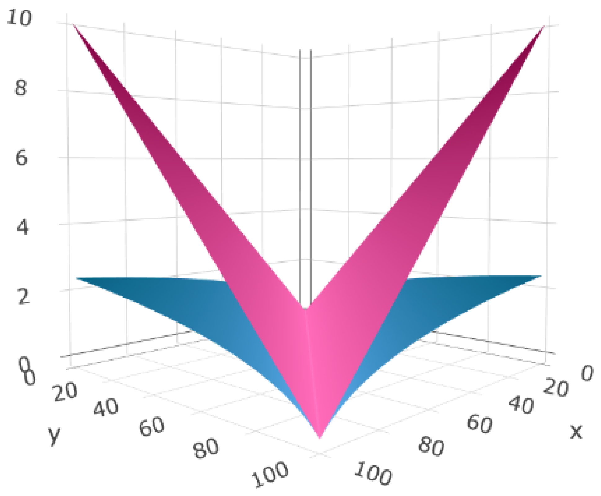
Figure 1. Comparison: d ( x , y ) (pink) and d ϕ ( x , y ) (blue).
Axioms 13 00192 g001
Figure 2. Visualization of the triangular inequality of both d and d ϕ : (a) d ( x , y ) (pink) versus d ( x , 0 ) + d ( 0 , y ) (blue) and (b) d ϕ ( x , y ) (pink) versus d ϕ ( x , 0 ) + d ϕ ( 0 , y ) (blue).
Axioms 13 00192 g002
Figure 3. Comparison of extension errors using McShane–Whitney formulas for different metrics: (a) results for d (yellow) and d ϕ (blue) and (b) results for d (yellow) and d ψ (blue).
Axioms 13 00192 g003
Figure 4. Comparison of extension errors using standard indices for different metrics: (a) results for d (yellow) and d ϕ (green) and (b) results for d (yellow) and d ψ (green).
Axioms 13 00192 g004
Figure 5. Comparison of extension errors using McShane–Whitney formulas for different metrics: (a) results for d (yellow) and d ϕ (green) and (b) results for d (yellow) and d ψ (green).
Axioms 13 00192 g005
Table 1. Examples of scores and indices for some cities.
CityWalk ScoreTransit ScoreBike ScoreI
New York8888.669.363
Los Angeles68.652.958.749
Chicago77.26572.257
Toronto6178.261?
Houston47.536.248.648
Montreal65.46772.6?
Table 2. Different procedures for the design of the function ϕ .
Function ϕ StandardMcShane–Whitney
Lipschitz ϕ -LipschitzLipschitz ϕ -Lipschitz
Mean RMSE138.4379.485.085.04
Median RMSE140.4981.255.125.05
Standard deviation24.118.780.610.60
Seconds per iteration1.039 × 10−33.316 × 10−11.513 × 10−33.330 × 10⁻¹
Table 3. Different procedures for the design of the function ψ .
Function ψ StandardMcShane–Whitney
Lipschitz ψ -LipschitzLipschitz ψ -Lipschitz
Mean RMSE138.4316.695.084.55
Median RMSE140.4916.505.124.47
Standard deviation24.111.520.610.63
Seconds per iteration1.039 × 10−33.000 × 10−11.513 × 10−33.013 × 10⁻¹
Table 4. Performance of ψ -metric models and other regression methods.
StandardMcShane–WhitneyNeural NetLinear
Mean RMSE16.694.554.4013.80
Median RMSE16.504.474.4213.65
Standard deviation1.520.630.463.25
Seconds per iteration3.000 × 10−13.013 × 10−11.923 × 10−14.341 × 10⁻³
Table 5. Ranking of Canadian cities.
RankingStandardMcShane–WhitneyNeural NetLinear
1VancouverMontrealVancouverVancouver
2TorontoVancouverTorontoToronto
3MontrealLongueuilMontrealMontreal
4BurnabyTorontoBurnabyBurnaby
5LongueuilSaskatoonLongueuilLongueuil
6MississaugaWinnipegOttawaOttawa
7WinnipegBurnabyWinnipegWinnipeg
8OttawaMississaugaMississaugaSurrey
9BramptonOttawaBramptonLaval
10QuebecBramptonQuebecMississauga
11SurreySurreyLavalKitchener
12LavalQuebecSurreyBrampton
13KitchenerEdmontonKitchenerHamilton
14CalgaryKitchenerCalgarySaskatoon
15SaskatoonWindsorGatineauCalgary
16MarkhamLavalMarkhamQuebec
17HamiltonHamiltonLondonWindsor
18EdmontonCalgaryHamiltonEdmonton
19LondonLondonEdmontonVaughan
20GatineauGatineauWindsorMarkham
21VaughanMarkhamVaughanLondon
22WindsorVaughanSaskatoonGatineau
Disclaimer/Publisher’s Note: The statements, opinions and data contained in all publications are solely those of the individual author(s) and contributor(s) and not of MDPI and/or the editor(s). MDPI and/or the editor(s) disclaim responsibility for any injury to people or property resulting from any ideas, methods, instructions or products referred to in the content.