Abstract
This paper proposes a novel slacks-based interval DEA approach that computes interval targets, slacks, and crisp inefficiency scores. It uses interval arithmetic and requires solving a mixed-integer linear program. The corresponding super-efficiency formulation to discriminate among the efficient units is also presented. We also provide a case study of its application to sustainable tourism in the Mediterranean region, assessing the sustainable tourism efficiency of twelve Mediterranean regions to validate the proposed approach. The inputs and outputs cover the three sustainability dimensions and include GHG emissions as an undesirable output. Three regions were found to be inefficient, and the corresponding inputs and output improvements were computed. A total rank of the regions was also obtained using the super-efficiency model.
MSC:
90B50; 90B99; 62C86; 62P25
1. Introduction
Data Envelopment Analysis (DEA) is a well-known non-parametric methodology to evaluate the efficiency of a set of Decision-Making Units (DMUs) that consume inputs (i.e., resources) to produce outputs (Zhu [1], Cooper et al. [2]). A Production Possibility Set (PPS) is derived from the observed inputs and outputs using certain axioms and the Principle of Minimum Extrapolation. This PPS contains all the feasible operating points. The non-dominated subset of the PPS is called the efficient frontier. A DMU is efficient if it lies on the efficient frontier. Otherwise, it is inefficient and can be projected onto a target operating point on the efficient frontier.
Regarding interval DEA, an extensive literature exists, mostly containing radial multiplier formulations (e.g., Despotis and Smirlis [3], Zhu [4]). Also, additive imprecise DEA approaches (e.g., Lee et al. [5]); FDH interval DEA models (e.g., Jahanshaloo et al. [6]); non-radial, non-oriented imprecise DEA approaches (e.g., Azizi et al. [7]); ideal point approaches (e.g., Jahanshahloo et al. [8]); inverted DEA approaches (e.g., Inuiguchi and Mizoshita [9]); interval DEA with negative data (e.g., Hatami-Marbini et al. [10]), flexible measure interval DEA approaches (e.g., Kordrostami and Jahani Sayyad Noveiri [11]); common weights imprecise DEA approaches (e.g., Hatami-Marbini et al. [12]); a three-Stage DEA model with interval inputs and outputs (e.g., Cheng et al. [13]); and a two-stage interval DEA (e.g., Kremantzis et al. [14]) exist. Applications include sustainable supply chain management under fuzzy data (see Azadi et al. [15]), the manufacturing industry (e.g., Wang et al. [16]), banks and bank branches (e.g., Jahanshaloo et al. [17], Inuiguchi and Mizoshita [9], Hatami-Marbini et al. [10]), and power plants (e.g., Khalili-Damghani et al. [18].
Super-efficiency, which aims to discriminate between efficient DMUs, was introduced by Andersen and Petersen [19] and has been continued by many authors such as Zhu [20], Seiford and Zhu [21], Zhong et al. [22], Li et al. [23], Esteve et al. [24], and Bolos et al. [25]. Although the initial super-efficiency approaches involved radial DEA models, a non-radial super-efficiency approaches based on the slacks-based measure of efficiency (super-SBM, [26]) as well as on the slacks-based measure of inefficiency (super-SBI, [27]) have also been proposed.
This paper considers inputs and outputs with continuous interval-valued data as a way of modelling mathematical uncertainty. The most similar DEA approach is that proposed by Arana-Jimenez et al. [28]. That work considers a hybrid scenario in which, in addition to integer interval data, some inputs or outputs are given as continuous intervals, but no super-efficiency model is proposed to rank or discriminate the efficient DMUs. In the present work, we focus on the continuous interval variables, with an enhanced formulation of the model given in [28] and a super-efficiency model. Thus, while [28] uses two phases for the slacks-based model under an additive and non-oriented approach, in the present work a one-phase interval Slack-based model is proposed. This is possible by using the difference of two intervals. Also, we propose a super-SBI interval DEA model to discriminate between efficient units.
To illustrate the usefulness of the proposed approach, we present an application to sustainable tourism. The first definitions of sustainable tourism focused on environmental and economic development, with community involvement included later [29]. The current sustainable tourism policy is often economic-growth oriented, with theoretical differences from sustainable development [30]. However, sustainable tourism management policies should maximise economic benefits while minimising adverse environmental impacts [31]. As regards the latter, GHG emissions are taken into account as an undesirable output, as discussed in the application section. As it is often done in the literature, this type of undsirable outputs can be treated as inputs (e.g., Tone and Tsutsui [26]; see also how [32,33] deal with water consumption and tourism energy, respectively). Finally, tourism sustainability should not only be based on a guide of good practices; it must also consider quantitative data that allow for evaluation to make decisions. In this regard, using indicators is a crucial tool that enables an assessment of the transition toward sustainability [34].
The structure of the paper is the following. Section 2 introduces the conventional crisp production possibility set (PPS) and corresponding crisp slacks-based DEA model for efficiency assessment. Section 3 introduces continuous intervals, especially arithmetic operations and partial orders. Section 4 presents the continuous interval PPS and corresponding interval slacks-based measure of inefficiency. In Section 5, a new enhanced interval slacks-based DEA approach is proposed. Section 6 presents the corresponding super-SBI interval DEA model to discriminate among efficient units. Section 7 presents the application to sustainable tourism, and finally, Section 8 summarises and concludes.
2. Crisp Production Possibility Set and Slack-Based Measure
Let us consider a set of n DMUs. For , each has m inputs and produces s outputs . In the classic Charnes et al. [35] DEA model, the production possibility set (PPS) or technology, denoted by T, satisfies the following axioms:
- (A1)
- Envelopment: , for all .
- (A2)
- Free disposability: , , , .
- (A3)
- Convexity: , then , for all .
- (A4)
- Scalability: , for all .
Following the minimum extrapolation principle (see [36]), the Constant Returns to Scale (CRS) and Variable Returns to Scale (VRS) DEA PPS are defined as the intersection of all the sets that satisfy axioms (A1)–(A4) or axioms (A1)–(A3), respectively, and can be expressed as
Let us also recall that a DMU p is said to be technically efficient if and only if for any such that and , then . This can be determined by solving the following normalised slacks-based DEA model
where , , are the intensity variables used for defining the corresponding efficient target of , and the constraint only applies in the VRS case, not in the CRS case. The inefficiency measures is units invariant and non-negative. Moreover, a is efficient if and only if .
3. Notation and Preliminaries
This paper deals with uncertainty in the data, and hence in the production possibility set, by modelling the corresponding inequality relationships using partial orders on integer intervals. This requires one to first introduce the following notation and results.
Let be the real number set. We denote by the family of all bounded closed intervals in . Some useful and necessary arithmetic operations for the purpose of this manuscript are introduced below (see, for instance, [37,38]).
Definition 1.
Let , and
- Addition:
- Opposite value:
- Substraction:
- Multiplication: .
- Multiplication by a scalar: for any , . For , .
Note that , in general. To overcome this issue, when the modelling requires it, we can define the -difference of two intervals A and B as follows ([37,38]):
Note that the -difference between an interval and itself is zero, i.e., . Furthermore, the -difference of two intervals always exists and is equal to
In the next section, we discuss the modelling with slack variables, and we will have to make use of the -difference between intervals to that end. It is also necessary to define a partial order relationship for integer intervals. In particular, we will adapt LU-fuzzy partial orders on intervals, which are well-known in the literature, (see, e.g., [37,39] and the references therein).
Definition 2.
Given two intervals , we say that:
- (i)
- if and only if and .
- (ii)
- if and only if and .
- (iii)
- if and only if and , or and .
Similarly, we define the relationships and for intervals, meaning and , respectively. We denote as the set of all non-negative intervals, i.e., .
4. Proposed Interval PPS and Slack-Based Measure of Inefficiency
Let us consider a set of N DMUs, for , with M inputs , with for all , and S outputs , with for all . The following hypotheses are analogous to (A1)–(A4) in Section 2 but consider interval inputs and outputs. We apply the corresponding interval arithmetic (Definition 1) and the partial order introduced in Definition 2:
- (B1)
- Envelopment: , for all .
- (B2)
- Free disposability: , , such that , , then .
- (B3)
- Convexity: , , then .
- (B4)
- Scalability: , and , then .
Theorem 1.
Under axioms (B1), (B2), (B3), and (B4), the CRS interval production possibility set PPS that results from the minimum extrapolation principle is
Proof.
This is similar to the proof given by Arana-Jimenez et al. [28]. □
In the case of discarding the scalability axiom, the corresponding PPS is as follows.
Theorem 2.
Under axioms (B1), (B2), and (B3), the VRS interval production possibility set PPS that results from the minimum extrapolation principle is
Proof.
This is similar to the proof given by Arana-Jimenez et al. [28]. □
Definition 3.
A is said to be technical efficient if and only if for any , with and implies .
Given the interval DEA technology , we can formulate the following slacks-based measure of the inefficiency interval DEA (IDEA) model with two phases.
If a is efficient, then (see Arana-Jimenez et al. [28]), but is not sufficient to guarantee that is efficient. Therefore, given the optimal solution of (4), , we need to formulate a phase II model to exhaust all remaining input and output slacks.
Given a with , then if and only if is efficient. In other words, a is efficient if and only if both and . Let be the optimal solution of (4), and let be the optimal solution of (5) for a given ; then, we can compute its input and output targets and as
As discussed in [28], considering new slacks , and in , or phase II, it was necessary to guarantee the efficiency of the corresponding DMU, as well as to compute its corresponding input and output targets. This is because the feasible slack improvements of the inequality constraints in (4) are not exhausted. Given two positive intervals , with , the positive interval upper slack such that , or the lower slack such that , do not necessarily exist. For instance, if we consider and , then . It is not possible to find a positive interval upper slack for which this equality holds. But from , we can find . Similarly, for and , the positive interval lower slack such that does not necessarily exist. But we find such that . Hence, given A and B two non-negative closed intervals, with , or always exists in such that or , as stated in the following proposition.
Proposition 1.
If , with , then exists such that or .
Proof.
On the one hand, following Stefanini and Arana [40], if , then . On the other hand, always exists such that
Since , then . In case (a), we have that , and if we define the Proposition holds. And in case (b), that is, , we can define , and the proof is complete. □
Proposition 2.
If , and such that , then .
Proof.
Since , and , then it follows that . □
Based on the previous propositions, we obtain the following useful results for formulating the forthcoming models.
Corollary 1.
Given , then if and only if exist such that , with or .
Proof.
It was shown in the proof of Proposition 1 that, if , there exists or , depending on the case (a) or (b), and we then have or , respectively. In the reverse direction, if , with , then, from Proposition 2, it follows that . □
Remark 1.
Given the Definition of the -difference, Equation (3), Corollary 1 actually implies that and , when (i.e., ), and and , otherwise (i.e., ).
Remark 2.
In the previous result, if A and B are crisp, with or , it implies that both and are crisp.
In the next section, we present a new enhanced interval DEA model based on applying these previous results to the (IDEA) model (4), aiming to unify the two phases (IDEA and PIDEA) by reducing the constraints to equalities from the start.
5. Enhanced Interval Slacks-Based Model
Let us recover the (IDEA) model (4) and take into account the previous discussions on its constraints, as well as Proposition 1. Thus, we propose the following Enhanced Inefficiency Non-Linear program (EINL) for our current DEA framework with interval data.
Comparing (IDEA) and (EINL), we tighten the input and output constraints to equality by considering low and upper slack variables on both sides of the constraints such that only one of them can be non-zero (as imposed in Equation (12)). Moreover, as stated in the following result, the inefficiency measure of any DMU under the (EINL) model is always higher than or equal to the inefficiency measure under (IDEA).
Proposition 3.
Given any , it holds that .
Proof.
Given the (EINL) model (8), efficient DMUs are expected to have a null inefficiency measure. We prove that only efficient DMUs satisfy the latter and, hence, that is a characterization of efficient DMUs.
Theorem 3.
is efficient if and only if .
Proof.
By contradiction, let us assume that . Then, if is not efficient exists such that and . As , then it also holds that and for some , with . Then, we have that and . Applying Corollary 1, we find some , with , such that , and , or . This is due to the ⪵ constraint derived from the Definition of efficiency. Similarly, in the case of the outputs, there are some , with , such that , and , or . By construction, it is straightforward that is a feasible solution of model , but its objective function (8) is strictly greater than zero, which is a contradiction of .
Now, let us suppose that is efficient, but . Then, there are some and , or and , for some . Or there are some , or , for some . We can then compute as for all , , and if , or if . Analogously, for all , with , and if , or if . By Definition, holds constraints (9) and (10); then, it belongs to the PPS, , and and , with . This implies a contradiction with the fact that is efficient. □
The previous mathematical program is nonlinear, but we can provide an equivalent linear program with variables leading to the following Enhanced Inefficiency Mix-Integer Linear program (EIMIL):
where Equations (16)–(20) are equivalent to the non-linear constrains (12), and are real positive constants and large enough. Recall that a number can be identified with an interval whose extremes are equal and coincide with such a number. Then, it can be compared with intervals via interval inequalities. Therefore, we can use, for example, , and . Another possibility is to set . In any case, (EIMIL) is an equivalent mix-integer linear program formulation to (EINL) and computes the same Enhanced Inefficiency Measure .
Let be an optimal solution of the model (15) for a given . Then, we can compute its input and output targets and as
The above Equations (21) and (22) are just the parametrizations derived from (9), and (10), respectively.
Theorem 4.
is efficient.
Proof.
By contradiction. Let be an optimal solution for model (15) for a given . From Equations (9), (10), (21) and (22), it follows that , and , (Proposition 2).
If were not efficient, there would be some such that , , with or , and , , for some , with . In summary, we have that
In the case of the inputs, applying Corollary 1, we can find some slacks , such that , and . Analogously, for the output case, we can find some slacks , such that , and . Moreover, given Remark 1 and that all intervals are in , it follows that
Analogously, for the output case, it holds that
Therefore we can find a feasible solution for model , , with a larger objective function value (15) than the optimum, , which is a contradiction. □
6. Super SBI Interval Model
Theorem 3 above indicates that all the efficient DMUs obtain the same zero inefficient measure. Hence, to discriminate between efficient units, a super-efficiency approach is considered. Super-efficiency as originally proposed by Andersen and Petersen [19] involved radial DEA models. The super-efficiency method applied to the Slack-based measure of inefficiency (SBI) metrics is appropriately called the super SBI model (see, e.g., Moreno and Lozano [27]). The idea behind the super-efficiency concept is to exclude the observation being benchmarked from the set of observations that define the technology. We present the proposed non-oriented super-SBI DEA model, which should be solved only for DMUs labeled efficient by the (EIMIL) model.
where are real positive constant numbers and large enough, as commented on before. The corresponding equivalent parametrized model is:
Let us note that when all data are crisp, then, from Remark 2, all slacks in (SuperEIMIL) are crisp and all interval equalities and inequalities become ordinary equalities and inequalities. Hence, in that case, defining , , the problem reduces to the conventional super-SBI DEA model, i.e.,
Before closing this section, let us mention that the PEIMIL model computes an inefficiency score so that the larger is, the more inefficient is. If we want to have a standardized efficiency score, we can use the optimal solution of that model (denoted with an asterisk) to compute an SBM efficiency score (e.g., Lozano and Soltani [41], Gutiérrez et al. [42]).
For an efficient , we can use the optimal solution of the S-PEIMIL model (denoted with a double asterisk) to compute a Super-SBM efficiency score (e.g., Soltani et al. [43]).
Note that . Moreover, is efficient. In that case, its corresponding Super-SBM efficiency score can be computed.
7. Application to Tourism
This section aims to assess, using the DEA methodology, the sustainability efficiency of tourism in the most important Mediterranean regions during 2019. According to the World Tourism Organization, sustainable development is “tourism that takes full account of its current and future economic, social, and environmental impacts, addressing the needs of visitors, the industry, the environment, and host communities.” Sustainability is usually represented in three fundamental pillars or dimensions: economic, social, and environmental [44]. Sustainability is a recent concept that is very important nowadays for the following reasons:
- It is key to preserving the planet;
- It helps to reduce pollution and conserve resources;
- It creates jobs and stimulates the economy;
- It improves public health;
- It protects biodiversity;
- It represents a development that is achievable with political will and public support.
On the other hand, tourism is considered one of the leading international commerce sectors and one of the primary sources of income for many developing countries. During the last decades, tourism has represented a significant global industry that has experienced continued growth. Actually, the number of tourist trips undertaken each year before the advent of COVID-19 exceeded the world’s population [45]. However, 2020 was a challenging year for most sectors because of the COVID-19 pandemic, and the tourism industry was affected notably.
Recent studies on sustainable tourism using DEA focus on the environmental effects and competitiveness of tourism. For example, Huang et al. [46] use SBM-DEA and Tobit’s regression to measure the efficiency of environmental training for diving tourists considering inputs such as education, Diver’s qualifications, or length of diving time and harmful environmental behaviors as outputs. Also, regarding eco-efficiency, Li et al. [23] use two DEA models (CCR and Panel Tobit) to assess the Chinese forest parks in 30 provinces of China, considering forest park employees, ecological tourism footprint, water consumption, and annual forest park tourism as inputs and total tourism revenue, SO2 emissions, and solid particulate emissions as outputs. To evaluate the impact of high-speed rail on the efficiency of low-carbon development in China, Li et al. [47] considered one input (namely, high-speed rail) and one output (namely, low-carbon tourism) using stochastic frontier analysis (SFA) in combination with BCC-DEA models. Bire [48] evaluated Indonesia’s Nusa Tenggara Timus province using Malmquist-DEA considering three inputs (namely, the number of accommodations, number of restaurants, and number of attractions) and one output (tourist visits) rethinking a new scenario for the regional tourism stakeholders. Pérez León et al. [49] proposed an index for measuring tourist destinations in the Caribbean Region, considering 27 indicators in four sub-indexes using DEA and goal programming to build composite indicators and measure the competitiveness of destinations. Flegl et al. [50] assessed the hospitality sector in Mexico using the CCR-DEA model with one input (number of rooms per hotel’s stars) and three outputs (occupancy rate, tourists arrivals, and related revenue per available room), obtaining high-efficiency results for national tourism and low-efficiency for international tourism and highlighting that the first is located in non-coastal states and the second in coastal states.
7.1. Variables and Data
The collection of data and variables related to the principles of sustainable tourism involves serious difficulties. The study by Rasoolimanesh [45] evaluating 97 papers on sustainable tourism with a focus on SDG indicators highlights that only a quarter of the studies take these indicators into account, showing the need to prioritize the creation of an internationally agreed on statistical framework to measure the impacts and dependence of tourism on the economy, society, and the environment. In short, the aim is to generate more solid data to quantify tourism sustainability. Another issue detected in this study is the frequency with which the data are published or the non-existence for determinate periods.
Therefore, the variables considered in this study (see Table 1 and Table 2, and Figure 1) are selected according to the dimensions of sustainability, which, together with the use of an interval variable and the proposed DEA model to handle it, represent a novelty in evaluating tourism efficiency in sustainability. The data refer to the year 2019, prior to the pandemic. We have used the Eurostat database and Regional databases from different Mediterranean regions. We would have liked to include additional regions and variables, but this was prevented by data availability. As a novelty in tourism studies, the variable Bed-places is of interval type, i.e., estimated as a confidence interval from the available data. Thus, with a focus on hotel infrastructure, the number of beds is considered an input, a variable also taken into account by other authors when carrying out efficiency measurements in the tourism field, such as [51] or [52]. However, our input comes from two databases with different data for some regions. Regarding the output variables, it is worth highlighting the tourism receipts (considered, for example, by [53]); regarding the social aspect, employment by gender (used, for example, by [54,55]); and finally, reagrding the environmental focus, the undesirable output GHG, a variable selected with a close relationship to tourism (used, for example, by [30,56,57]).

Table 1.
Data Description of the input and outputs for the tourism application.
Table 2.
Input and Outputs data.
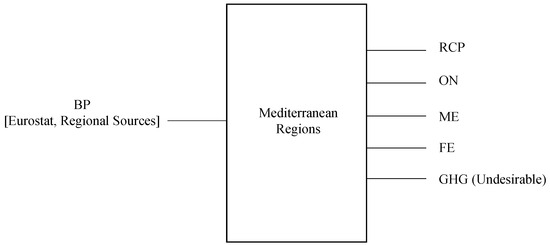
Figure 1.
Input and outputs considered in this sustainable tourism application.
Finally, the selection of variables aligns with the 2030 Agenda for Sustainable Development objectives, in particular, objectives 8 and 9 (Economic Growth and Industry, Innovation, and Infrastructure) concerning economic variables; Objective 5 (Gender Quality) in the social aspect, with references to employment variables; and Objectives 12 and 13 (Responsible Consumption and Production & Climate Action, respectively) for the environmental variable GHG.
7.2. Results and Discussion
The inefficiency scores of the proposed (EIMIL) DEA model with its corresponding targets and slacks intervals are shown in Table 3. Because of the relatively small dataset, only three DMUs are inefficient: Nisia Aigaiou-Kriti, Cyprus, and the Provence-Alpes-Côte d’Azur. That is why, in order to rank the DMUs fully, the super-SBI interval DEA model (S-PEIMIL) has been solved. The corresponding super-inefficiency scores and the final ranking are also shown.
Table 3.
Results from the (EIMIL) (15) (second column) and (S-EIMIL) (37) (third column) models, respectively. The SBM (48) and Super-SBM (49) efficiency scores are given in the fourth and fifth columns, and the corresponding ranking is given in the sixth column. We also include the slacks and the targets. Only the inefficient DMUs have non-zero slacks. For clarity, we represent those null interval slacks as zero, i.e., .
Note that, regarding sustainable tourism, the two Greek regions considered in this study have disparate results, with Attiki and Nisia Aigaiou (Kriti) at the top and bottom of the ranking, respectively. The second-best score is for Cataluña, with similar scores as the Croatian region Jadranska Hrvatska, followed by the Italian regions of Campania and Veneto. On the bottom side, Cyprus and the Provence-Alpes-Côte d’Azur, in addition to Kriti, are inefficient.
Regarding inefficient regions, Nisia Aigaiou (Kriti) needs to increase receipts by around 28% and female and male employment by up to 494% and 447%, respectively, to reach the frontier of tourism sustainability. Regarding the number of beds, the interval variable has an excess of 28% and 12% with respect to their current value according to the Eurostat and the regional databases, respectively. Similarly, Provence-Alpes-Côte d’Azur has margins for improvement of 248% and 195% for female and male employment, respectively, and for increasing the receipts by 10%. The interval input variable shows zero slacks for the Eurostat database and around 5% slack for the regional database. Finally, Cyprus is the only study area with a margin of improvement in greenhouse gas emissions. Namely, they could decrease by 46%. It also has margins of improvement of 246% and 305% in female and male employment, respectively, and of 10% in overnight stays. As for the BP interval input, the slack is zero for the Eurostat database and around 5% for the regional database.
The regions of Nisia Aigaiou (Kriti) and Provence-Alpes-Côte d’Azur, despite showing efficiency in overnight stays and GHG emissions, to reach the frontier of tourism sustainability must implement transformation policies, such as improvements in the tourism offer with a focus on improving the deficiencies shown in income, which entail the creation of new tourism companies to mitigate employment deficiencies, as well as the reduction in visitors with an increase in their tourist spending to alleviate excesses of numbers of beds, betting on higher quality tourism. For its part, the Cypriot region, despite remaining efficient in tourism revenue, also must implement different transformation policies—in this case, like the other two inefficient regions of the study, betting on quality tourism focused on increasing overnight stays and creating tourism companies to alleviate deficiencies in employment and minimally reducing the number of visitors. No less important, being the only region showing deficiencies in the environmental dimension, it would be advisable to apply and implement environmental regulations that would allow for a reduction of almost the 50% necessary to reach the frontier of tourism sustainability.
Besides the two-stage approach [27] requiring two phases to achieve the same result or efficiency classification as in the current work, it cannot provide a full ranking among the efficient DMUs since it does not include the super-efficiency score. These scores, (48) and (49), are also included in the results of the case study shown in Table 3.
For comparison purposes, Table 4 shows the corresponding efficiency scores and computed by the two-stage approach [28], as well as the overall efficiency intervals computed by the non-oriented SBM model for interval data proposed by Azizi et al. [7], together with the ranking they provide. We note that, despite the fact that the two-stage approach [28] requires two phases to achieve the same result or efficiency classification as in the current work, it cannot provide a full ranking among the efficient DMUs since it does not include the super-efficiency score. In the case of [7], their method computes an interval measure of efficiency, although it does not compute targets. Their approach uses a preference-degree approach for comparing and ranking the DMUs. The corresponding ranking computed by these authors for this dataset is also included in Table 4. Their ranking and the proposed approach are not correlated (Spearman correlation coefficient = −0.056). This is undoubtedly due to their considering a double frontier approach.
Table 4.
Comparison with other models from the Literature.
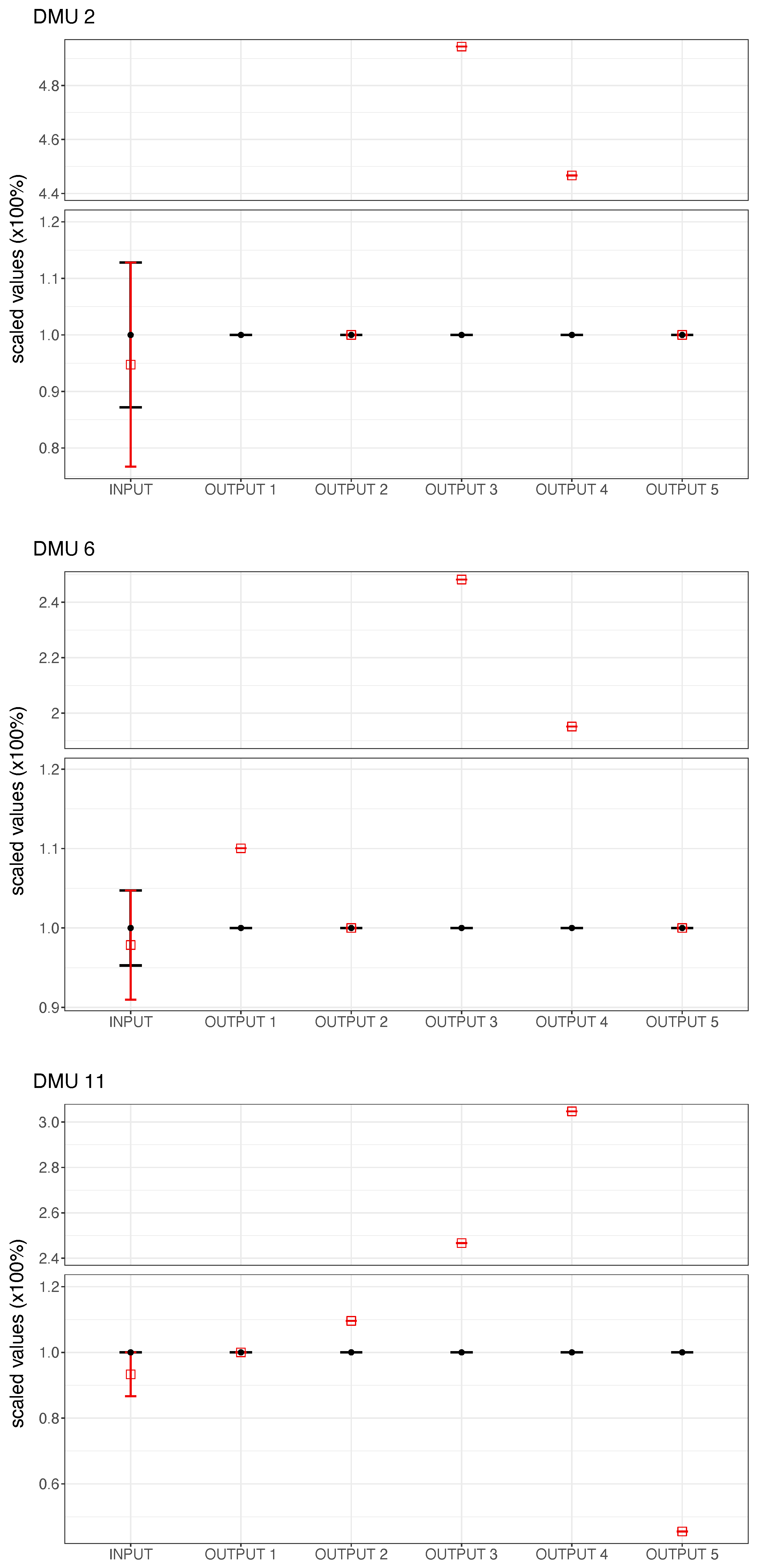
Figure 2 shows the observed and the target inputs and outputs for the three inefficient DMUs. The values are scaled by the corresponding observed data to facilitate their comparison. Note that, as the fifth output is undesirable, the corresponding targets stayed the same or were reduced. Note also that, in this application, only the input variable involves interval data.
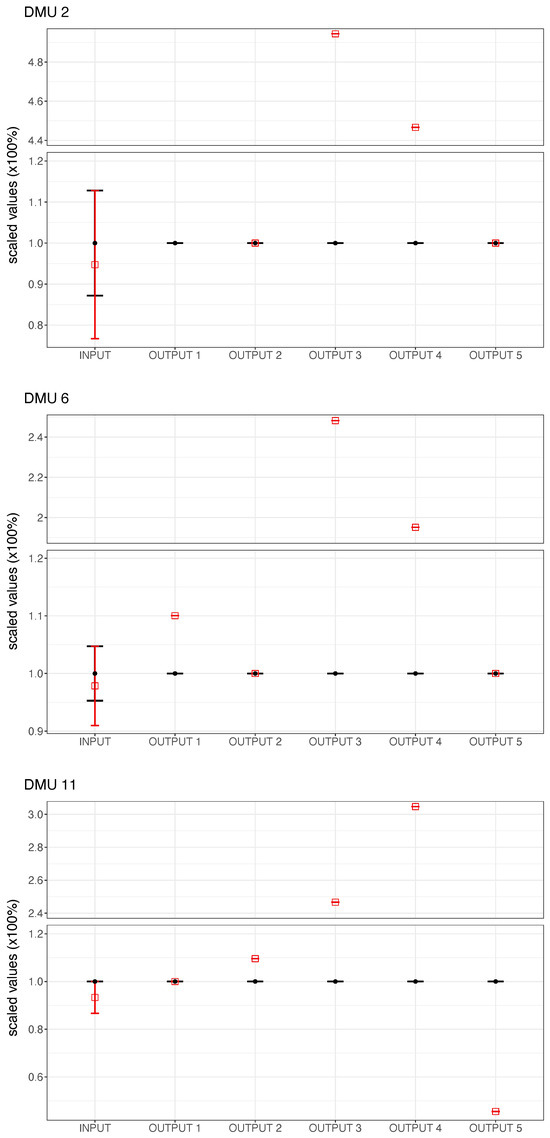
Figure 2.
Input and outputs targets for the three inefficient DMUs: Nisia Aigaiou, Kriti (labeled DMU 2), Provence-Alpes-Côte d’Azur (labeled DMU 6), and Cyprus (labeled DMU 11).
8. Conclusions
This paper has proposed a new interval-valued DEA approach and associated slacks-based inefficiency measures. It requires solving a mixed-integer linear program that allows one to compute the corresponding input and output targets. A super-efficiency version of the model has also been formulated in case a full ranking of the DMUs is desired.
An application for sustainable tourism efficiency assessment has also been presented. The input and output variables span the three sustainability dimensions, including the environmental dimension, represented by GHG emissions from tourism activities. The need to apply an interval DEA approach comes from the fact that for the input variable (Bed-places), the data come from two different data sources, and in some cases, the corresponding values do not coincide. This is something that often occurs in practice. In order to avoid loss of information, it was decided to represent that variable as an interval using the values from the two sources as limits. The proposed approach has handled this type of variable computing inefficiency scores and targets for all the DMUs. In this application, given the small dataset available, many DMUs were labeled as efficient, which also required solving the corresponding super-efficiency DEA model.
As a continuation of this research, we plan to apply this approach to other sectors (e.g., healthcare, transportation, etc.) where input and output interval data can occur. Also, the proposed approach could be extended to Network DEA scenarios, i.e., production systems involving multiple interconnected processes.
Author Contributions
Conceptualization, methodology, validation, formal analysis, investigation, and writing, M.A.-J. and M.C.S.-G.; resources, data curation, and writing—original draft preparation, J.L.-R.; software, M.C.S.-G.; supervision, M.A.-J.; and writing—review and editing, A.Y. and S.L. All authors have read and agreed to the published version of the manuscript.
Funding
This research was funded by Spanish Ministry of Science and Innovation grants PID2019-105824GB-I00 and PID2021-124981NB-I00.
Data Availability Statement
The data presented in this study are available on request from the corresponding author (privacy).
Acknowledgments
The first and second authors are partially supported by grant PID2019-105824GB-I00. The fifth author acknowledges the financial support of the Spanish Ministry of Science and Innovation, grant PID2021-124981NB-I00.
Conflicts of Interest
The authors declare no conflicts of interest.
Abbreviations
The following abbreviations are used in this manuscript:
| DEA | Data Envelopment Analysis |
| DMUs | Decision-Making Units |
| EIMIL | Enhanced Inefficiency Mix-Integer Linear program |
| SBI | Slacks-based measure of inefficiency |
References
- Zhu, J. Quantitative Models for Performance Evaluation and Benchmarking; International Series in Operations Research & Management Science; Kluwer Academic: Tucson, AZ, USA, 2002. [Google Scholar]
- Cooper, W.W.; Seiford, L.M.; Zhu, J. Handbook on Data Envelopment Analysis; International Series in Operations Research Management Science; Kluwer Academic: Tucson, AZ, USA, 2004. [Google Scholar]
- Despotis, D.K.; Smirlis, Y.G. Data envelopment analysis with imprecise data. Eur. J. Oper. Res. 2002, 140, 24–36. [Google Scholar] [CrossRef]
- Zhu, J. Imprecise data envelopment analysis (IDEA): A review and improvement with an application. Eur. J. Oper. Res. 2003, 144, 513–529. [Google Scholar] [CrossRef]
- Lee, Y.K.; Park, K.S.; Kim, S.H. Identification of inefficiencies in an additive model based IDEA (imprecise data envelopment analysis). Comput. Oper. Res. 2002, 29, 1661–1676. [Google Scholar] [CrossRef]
- Jahanshahloo, G.; Lofti, F.H.; Moradi, M. Sensitivity and stability analysis in DEA with interval data. Appl. Math. Comput. 2004, 156, 463–477. [Google Scholar] [CrossRef]
- Azizi, H.; Kordrostami, S.; Amirteimoori, A. Slacks-based measures of efficiency in imprecise data envelopment analysis: An approach based on data envelopment analysis with double frontiers. Comput. Ind. Eng. 2015, 79, 42–51. [Google Scholar] [CrossRef]
- Jahanshahloo, G.; Lotfi, F.H.; Rezaie, V.; Khanmohammadi, M. Ranking DMUs by ideal points with interval data in DEA. Appl. Math. Model. 2011, 35, 218–229. [Google Scholar] [CrossRef]
- Inuiguchi, M.; Mizoshita, F. Qualitative and quantitative data envelopment analysis with interval data. Ann. Oper. Res. 2011, 195, 189–220. [Google Scholar] [CrossRef]
- Hatami-Marbini, A.; Emrouznejad, A.; Agrell, P.J. Interval data without sign restrictions in DEA. Appl. Math. Model. 2014, 38, 2028–2036. [Google Scholar] [CrossRef]
- Kordrostami, S.; Noveiri, M.J.S. Evaluating the performance and classifying the interval data in data envelopment analysis. Int. J. Manag. Sci. Eng. Manag. 2014, 9, 243–248. [Google Scholar] [CrossRef]
- Hatami-Marbini, A.; Beigi, Z.G.; Fukuyama, H.; Gholami, K. Modeling Centralized Resources Allocation and Target Setting in Imprecise Data Envelopment Analysis. Int. J. Inf. Technol. Decis. Mak. 2015, 14, 1189–1213. [Google Scholar] [CrossRef]
- Cheng, G.Q.; Wang, L.; Wang, Y.M. An Extended Three-Stage DEA Model with Interval Inputs and Outputs. Int. J. Comput. Intell. Syst. 2020, 14, 43. [Google Scholar] [CrossRef]
- Kremantzis, M.D.; Beullens, P.; Klein, J. A ranking framework based on interval self and cross-efficiencies in a two-stage DEA system. RAIRO—Oper. Res. 2022, 56, 1293–1319. [Google Scholar] [CrossRef]
- Azadi, M.; Jafarian, M.; Saen, R.F.; Mirhedayatian, S.M. A new fuzzy DEA model for evaluation of efficiency and effectiveness of suppliers in sustainable supply chain management context. Comput. Oper. Res. 2015, 54, 274–285. [Google Scholar] [CrossRef]
- Wang, Y.M.; Greatbanks, R.; Yang, J.B. Interval efficiency assessment using data envelopment analysis. Fuzzy Sets Syst. 2005, 153, 347–370. [Google Scholar] [CrossRef]
- Jahanshahloo, G.; Lotfi, F.H.; Malkhalifeh, M.R.; Namin, M.A. A generalized model for data envelopment analysis with interval data. Appl. Math. Model. 2009, 33, 3237–3244. [Google Scholar] [CrossRef]
- Khalili Damghani, K.; Haji Sami, E. Productivity of steam power-plants using uncertain DEA-based Malmquist index in the presence of undesirable outputs. Int. J. Inf. Decis. Sci. 2018, 10, 162. [Google Scholar] [CrossRef]
- Andersen, P.; Petersen, N.C. A Procedure for Ranking Efficient Units in Data Envelopment Analysis. Manag. Sci. 1993, 39, 1261–1264. [Google Scholar] [CrossRef]
- Zhu, J. Data Envelopment Analysis. In International Series in Operations Research & Management Science; International Series in Operations Research & Management Science; Springer International Publishing: Cham, Switzerland, 2014; pp. 1–9. [Google Scholar]
- Seiford, L.M.; Zhu, J. Infeasibility Of Super-Efficiency Data Envelopment Analysis Models. INFOR Inf. Syst. Oper. Res. 1999, 37, 174–187. [Google Scholar] [CrossRef]
- Zhong, K.; Wang, Y.; Pei, J.; Tang, S.; Han, Z. Super efficiency SBM-DEA and neural network for performance evaluation. Inf. Process. Manag. 2021, 58, 102728. [Google Scholar] [CrossRef]
- Li, D.; Zhai, Y.; Tian, G.; Mendako, R.K. Tourism Eco-Efficiency and Influence Factors of Chinese Forest Parks under Carbon Peaking and Carbon Neutrality Target. Sustainability 2022, 14, 13979. [Google Scholar] [CrossRef]
- Esteve, M.; Aparicio, J.; Rodriguez-Sala, J.J.; Zhu, J. Random Forests and the measurement of super-efficiency in the context of Free Disposal Hull. Eur. J. Oper. Res. 2023, 304, 729–744. [Google Scholar] [CrossRef]
- Bolós, V.J.; Benítez, R.; Coll-Serrano, V. Continuous models combining slacks-based measures of efficiency and super-efficiency. Cent. Eur. J. Oper. Res. 2022, 31, 363–391. [Google Scholar] [CrossRef]
- Tone, K. A slacks-based measure of super-efficiency in data envelopment analysis. Eur. J. Oper. Res. 2002, 143, 32–41. [Google Scholar] [CrossRef]
- Moreno, P.; Lozano, S. Super SBI Dynamic Network DEA approach to measuring efficiency in the provision of public services. Int. Trans. Oper. Res. 2016, 25, 715–735. [Google Scholar] [CrossRef]
- Arana-Jiménez, M.; Sánchez-Gil, M.; Younesi, A.; Lozano, S. Integer interval DEA: An axiomatic derivation of the technology and an additive, slacks-based model. Fuzzy Sets Syst. 2021, 422, 83–105. [Google Scholar] [CrossRef]
- Hardy, A.; Beeton, R.J.S.; Pearson, L. Sustainable Tourism: An Overview of the Concept and its Position in Relation to Conceptualisations of Tourism. J. Sustain. Tour. 2002, 10, 475–496. [Google Scholar] [CrossRef]
- Guo, Y.; Jiang, J.; Li, S. A Sustainable Tourism Policy Research Review. Sustainability 2019, 11, 3187. [Google Scholar] [CrossRef]
- Nepal, R.; al Irsyad, M.I.; Nepal, S.K. Tourist arrivals, energy consumption and pollutant emissions in a developing economy–implications for sustainable tourism. Tour. Manag. 2019, 72, 145–154. [Google Scholar] [CrossRef]
- Ma, H.; Geng, B.; Fu, Y.; Sun, Y.; Sun, Z. Efficiency Analysis of Industrial Water Treatment in China Based on Two-stage Undesirable Fixed-sum Output DEA Model. J. Syst. Sci. Inf. 2021, 9, 660–680. [Google Scholar] [CrossRef]
- Chen, Y.; Zhu, Z.; Zhuang, L. Exploring the Ecological Performance of China’s Tourism Industry: A Three-Stage Undesirable SBM-DEA Approach with Carbon Footprint. Int. J. Environ. Res. Public Health 2022, 19, 15367. [Google Scholar] [CrossRef]
- Navarro, J.L.A.; Martínez, M.E.A.; Jiménez, J.A.M. An approach to measuring sustainable tourism at the local level in Europe. Curr. Issues Tour. 2020, 23, 423–437. [Google Scholar] [CrossRef]
- Charnes, A.; Cooper, W.; Rhodes, E. Measuring the efficiency of decision making units. Eur. J. Oper. Res. 1978, 2, 429–444. [Google Scholar] [CrossRef]
- Banker, R.D.; Charnes, A.; Cooper, W.W. Some Models for Estimating Technical and Scale Inefficiencies in Data Envelopment Analysis. Manag. Sci. 1984, 30, 1078–1092. [Google Scholar] [CrossRef]
- Stefanini, L.; Bede, B. Generalized Hukuhara differentiability of interval-valued functions and interval differential equations. Nonlinear Anal. Theory Methods Appl. 2009, 71, 1311–1328. [Google Scholar] [CrossRef]
- Stefanini, L. A generalization of Hukuhara difference and division for interval and fuzzy arithmetic. Fuzzy Sets Syst. 2010, 161, 1564–1584. [Google Scholar] [CrossRef]
- Wu, H.C. The optimality conditions for optimization problems with convex constraints and multiple fuzzy-valued objective functions. Fuzzy Optim. Decis. Mak. 2009, 8, 295–321. [Google Scholar] [CrossRef]
- Stefanini, L.; Arana-Jiménez, M. Karush–Kuhn–Tucker conditions for interval and fuzzy optimization in several variables under total and directional generalized differentiability. Fuzzy Sets Syst. 2019, 362, 1–34. [Google Scholar] [CrossRef]
- Lozano, S.; Soltani, N. DEA target setting using lexicographic and endogenous directional distance function approaches. J. Product. Anal. 2018, 50, 55–70. [Google Scholar] [CrossRef]
- Gutiérrez, E.; Lozano, S.; Guillén, J. Efficiency data analysis in EU aquaculture production. Aquaculture 2020, 520, 734962. [Google Scholar] [CrossRef]
- Soltani, N.; Yang, Z.; Lozano, S. Ranking decision making units based on the multi-directional efficiency measure. J. Oper. Res. Soc. 2021, 73, 1996–2008. [Google Scholar] [CrossRef]
- Lozano, R. Envisioning sustainability three-dimensionally. J. Clean. Prod. 2008, 16, 1838–1846. [Google Scholar] [CrossRef]
- Rasoolimanesh, S.M.; Ramakrishna, S.; Hall, C.M.; Esfandiar, K.; Seyfi, S. A systematic scoping review of sustainable tourism indicators in relation to the sustainable development goals. J. Sustain. Tour. 2020, 31, 1497–1517. [Google Scholar] [CrossRef]
- Huang, C.W.; Ng, E.; Fang, W.T.; Lo, L. Assessing the Effectiveness of Environmental Training for Diving Tourists Using the DEA Model. Sustainability 2022, 14, 1639. [Google Scholar] [CrossRef]
- Li, Q.; Chen, S.; He, L.; Huang, G.; Li, R.; Pan, W. Application of Two-Stage Network Super-Efficiency DEA to Efficiency Analysis of Chinese Commercial Banks. J. Math. 2022, 2022, 1–7. [Google Scholar] [CrossRef]
- Bire, R.B. Mapping destination competitiveness in Indonesia’s Nusa Tenggara Timur (NTT) province: A Malmquist–data envelopment analysis approach. Reg. Sci. Policy Pract. 2021, 13, 820–834. [Google Scholar] [CrossRef]
- León, V.E.P.; Pérez, F.; Rubio, I.C.; Guerrero, F.M. An approach to the travel and tourism competitiveness index in the Caribbean region. Int. J. Tour. Res. 2020, 23, 346–362. [Google Scholar] [CrossRef]
- Flegl, M.; Cerón-Monroy, H.; Krejčí, I.; Jablonský, J. Estimating the hospitality efficiency in Mexico using Data Envelopment Analysis. OPSEARCH 2022, 60, 188–216. [Google Scholar] [CrossRef]
- Sellers-Rubio, R.; Casado-Díaz, A.B. Analyzing hotel efficiency from a regional perspective: The role of environmental determinants. Int. J. Hosp. Manag. 2018, 75, 75–85. [Google Scholar] [CrossRef]
- Solana-Ibáñez, J.; Caravaca-Garratón, M.; Para-González, L. Two-Stage Data Envelopment Analysis of Spanish Regions: Efficiency Determinants and Stability Analysis. Contemp. Econ. 2016, 10, 259–274. [Google Scholar] [CrossRef]
- Soysal-Kurt, H. Measuring Tourism Efficiency of European Countries by Using Data Envelopment Analysis. Eur. Sci. Journal, ESJ 2017, 13, 31. [Google Scholar] [CrossRef]
- Kumar, S. Sustainability Analysis of Tourism in India: Data Envelopment Analysis Approach. Int. J. Virtual Communities Soc. Netw. 2018, 10, 33–45. [Google Scholar] [CrossRef]
- Radovanov, B.; Dudic, B.; Gregus, M.; Marcikic Horvat, A.; Karovic, V. Using a Two-Stage DEA Model to Measure Tourism Potentials of EU Countries and Western Balkan Countries: An Approach to Sustainable Development. Sustainability 2020, 12, 4903. [Google Scholar] [CrossRef]
- Wang, R.; Xia, B.; Dong, S.; Li, Y.; Li, Z.; Ba, D.; Zhang, W. Research on the Spatial Differentiation and Driving Forces of Eco-Efficiency of Regional Tourism in China. Sustainability 2020, 13, 280. [Google Scholar] [CrossRef]
- Gao, J.; Shao, C.; Chen, S. Evolution and Driving Factors of the Spatiotemporal Pattern of Tourism Efficiency at the Provincial Level in China Based on SBM–DEA Model. Int. J. Environ. Res. Public Health 2022, 19, 10118. [Google Scholar] [CrossRef] [PubMed]

Disclaimer/Publisher’s Note: The statements, opinions and data contained in all publications are solely those of the individual author(s) and contributor(s) and not of MDPI and/or the editor(s). MDPI and/or the editor(s) disclaim responsibility for any injury to people or property resulting from any ideas, methods, instructions or products referred to in the content. |
© 2024 by the authors. Licensee MDPI, Basel, Switzerland. This article is an open access article distributed under the terms and conditions of the Creative Commons Attribution (CC BY) license (https://creativecommons.org/licenses/by/4.0/).