Article

Analysis of Epidemic Models in Complex Networks and Node Isolation Strategie Proposal for Reducing Virus Propagation

by
Carlos Rodríguez Lucatero
Departamento de Tecnologías de la Información, Universidad Autónoma Metropolitana Unidad Cuajimalpa, Torre III, 6to piso, Av. Vasco de Quiroga 4871, Col. Santa Fe Cuajimalpa, Alcaldia Cuajimalpa de Morelos, Mexico City CP 05348, Mexico
Axioms 2024, 13(2), 79; https://doi.org/10.3390/axioms13020079
Submission received: 3 November 2023 / Revised: 24 December 2023 / Accepted: 28 December 2023 / Published: 25 January 2024
(This article belongs to the Special Issue Computer Methods in Mathematical Epidemiology)

Abstract

:
Many models of virus propagation in Computer Networks inspired by epidemic disease propagation mathematical models that can be found in the epidemiology field (SIS, SIR, SIRS, etc.) have been proposed in the last two decades. The purpose of these models has been to determine the conditions under which a virus becomes rapidly extinct in a network. The most common models of virus propagation in networks are SIS-type models or their variants. In such models, the conditions that lead to a rapid extinction of the spread of a computer virus have been calculated and its dependence on some parameters inherent to the mathematical model has been observed. In this article, we will try to analyze a particular SIS-type model proposed in the past by Chakrabarti as well as an SIRS-type variation of this model proposed in the past by myself. I will show through simulations the influence that the topology of a network has on the dynamics of the spread of a virus in different network types. In the recent past, there have been interesting articles that demonstrate the relationship between the eigenvalue λ 1 of the adjacency matrix and the reduction in the spread of a virus in a network. From this, the minimization of the spectral radius strategies by edge suppression has been proposed. This problem is NP-complete in its general case and for this reason, heuristic algorithms have been proposed. In this article, I will perform simulations of an SIS-type model in topologies with the same number of nodes but with different structures to compare their epidemic behavior. The simulations will show that regular topologies with small node degrees, i.e., of degree 4, as is the case of the topology that I call Lattice4, have favorable behavior in terms of the fast extinction property, with respect to other denser and less regular topologies such as the binomial topologies as well as Power law topologies. Based on the results of the simulations, my contribution will consist of proposing, as a node isolation strategy, a transformation of the original topology into an approximately regular topology by edge elimination. Although such a transformed topology is not optimal in terms of reducing the propagation of a virus, it induces the rapid extinction of the virus in the network.
MSC:
05C82; 05C85; 93A30; 93B60; 68R10

1. Introduction

I would like to begin this section of the article by mentioning the theoretical character of this research and mentioning that for this reason no real data are presented. However, it is also worth mentioning that the present research may have practical applications that could be explored in the future. The issue of virus spread as well as the conditions under which it is extinguished or has contaminated most of the nodes of a computer network has been studied for at least two decades. The models that have been proposed are based on mathematical models of virus spread in the field of epidemiology [1,2]. These models are differential equations that try to capture the dynamics of a virus spread in order to answer questions such as, How long will it take for the epidemic to go extinct? At what point will it peak? Will it remain endemic at a certain level of infection? Will it generate permanent immunity to those who suffer from the disease?
These mathematical models emerged from the area of epidemiology and are known as compartmental because they model the process as states in which an individual finds himself during an epidemic and transition probabilities between these states. In other words, an individual can be susceptible, exposed, infected, or recovered from a virus, and these states are modeled as compartments. From these compartments and the transition probabilities between them, relationships can be established in the form of differential equations that describe the dynamics of the spread of a disease [3]. The compartments used by one of those models depend on the disease to be modeled, since there are diseases that produce permanent immunity such as measles, while some diseases such as seasonal influenza do not produce permanent immunity. The spread of disease in epidemic processes shares similarities with the massive attacks on a computer network, and therefore, some ideas from the mathematical modeling of epidemics served as the basis for models of virus spread in computer networks. However, it is worth mentioning that some problems that arise in the study of the spread of viruses in computer networks, as well as their respective solutions, may be useful for epidemiology. There have been very famous massive attacks on computer networks. One of the first denial-of-service-type attacks turned 20 on 7 February 2020, and was conducted by a 15-year-old Canadian hacker whose pseudonym was Mafiaboy and whose real name is Michael Calce. Denial of service type attacks consist of sending a huge number of service request packets to a target server in such a way that it exceeds the capacity of said server to respond to so many orders, thus causing it to crash. This massive attack revealed the vulnerability of networks such as the internet and led to a study of the causes of said vulnerability and and gave birth to a new type of computer virus. This vulnerability aroused the interest of researchers in the field of network security and they realized that certain topologies favored faster dissemination of information than others or that a certain type of interconnection kept the nodes of a network connected despite the fact that some lines were faulty. Some studies showed that the type of interconnection structures that are formed in networks such as the Internet, Facebook, or Twitter have similar characteristics and that they produce the appearance of giant components as well as the phenomenon of small worlds. The formalization of the relationship between the topology of the networks and the appearance of the aforementioned phenomena uses the theory of random graphs as a mathematical tool. The type of interconnection structures that are formed in social networks such as Facebook, Twitter and the Internet have been characterized as particular graphs whose distribution of degrees of the nodes is known as the type of power laws due to the mathematical form that expresses said distribution which in algebraic terms would be p k C k γ with 2 < γ 3 . The formation of networks with these topological characteristics is closely related to the type of connection protocol used and is known as preferential attachment. It is said that this type of network is both robust and vulnerable since if they were removed by randomly choosing more than 90 % of the edges of the associated graph, it would continue to be a connected graph, while if they were removed by strategically choosing a number small number ( 2.3 % ) of vertices of the associated graph, the original graph would be split into unconnected components [4]. Networks that have these characteristics of node degree distribution allow phenomena such as small worlds to appear due to the fact that their diameter is generally smaller than that of other graphs with other topologies. This also has an impact on the speed with which messages are spread and I will illustrate that through simulations in the following sections of the present article.

2. Epidemiology Mathematical Models

Epidemics have been with humans for a long time. One of the oldest diseases is leprosy. Another disease that devastated Europe in the Middle Ages was the Black Death. Little was known about these diseases and how to cure them. In these circumstances, it was necessary to try to understand the way in which the epidemic process was developing in order to at least stay safe from them. In the absence of objective knowledge based on science, there was a tendency to believe that such calamities were divine punishments. Perhaps since those times the most helpful strategy consisted of isolating oneself. Some diseases such as smallpox have been treated since ancient times using the variolation method, which consisted of inoculating the scales of a sick patient in a healthy individual and observing that this allowed said individual to acquire a certain type of immune protection. The knowledge of this empirical method of immunization was imported to Europe from the colonies and later served as a starting point for the development of vaccines for this disease [3]. In search of answers to questions that disturbed humanity over the years, one of the first mathematical models of the spread of smallpox appeared in the year 1760 and was proposed by Daniel Bernoulli  [5]. Later, deterministic mathematical models of virus spread began to be developed at the beginning of the 20th century. In 1906 a discrete time model was formulated and analyzed for measles epidemics [6]. In 1911 some differential equations-based models for malaria were formulated in [7,8,9,10].
Mathematical models of this type of phenomenon clarify which are the important parameters to take into account to obtain concepts such as thresholds, basic reproduction numbers, number of contacts and replacement numbers. This in turn allows us to make computer simulations. Having the information provided by epidemiological models helps to know what data must be collected in an epidemic, identify trends, make estimates and calculate uncertainties in these estimates. Later, in 1926, models were formulated from which thresholds could be calculated or an epidemic outbreak appears and this happens when the number of susceptible reaches a critical value [8,11,12]. The model presented in [12] is a reference in the modeling with non-linear dynamic systems of the phenomenon of virus propagation in networks. This type of model is known as composed by compartments since it conceives the states through which an individual passes during an epidemic as boxes or compartments. The compartments are labeled by the letters M , S , E , I , R and S that cover the different characteristics that one may have, such as having generated antibodies from the mother’s womb by maternal transmission, being susceptible, being exposed, being infected and having recovered from the disease, respectively. It is entered vertically either to the state M or to the state S and it is exited vertically when passing to a state of death. There are horizontal transfers between state M to S, from S to E, from E to I and from I to R as it is shown in Figure 1. Some of these compartments will be present in a specific model and others will not be, depending on the particular characteristics of the disease to be modeled. For instance, if the disease to be modeled produces permanent immunity, does not have a passive immunity transmitted by the mother and there is no incubation period, then the compartments that will be present are S , I  R (Susceptible, Infected and Recovered) and will be called a S I R -model.
In mathematical epidemic models, the threshold for many epidemiological models is the reproduction number R 0 , which is defined as the average number of secondary infections produced when an infected individual is introduced into a host population where everyone is susceptible. Normally, R 0 is bigger than 1. When the time span of the process is quite long, the model is called endemic otherwise it is called epidemic. In the case of endemic models, factors such as population growth or population decrease must be included and it affects the calculation of R 0 . In other models, the demographic age structure is taken into account and this can change the calculation of R 0 as well. On the other hand, if  R 0 < 1 the epidemic dies out quickly and does not emerge in a large population. In the next subsection, I will formulate the classic mathematical epidemic models known as SIR and SIS and show how they work with some simple simulations that I have implemented in MATLAB.

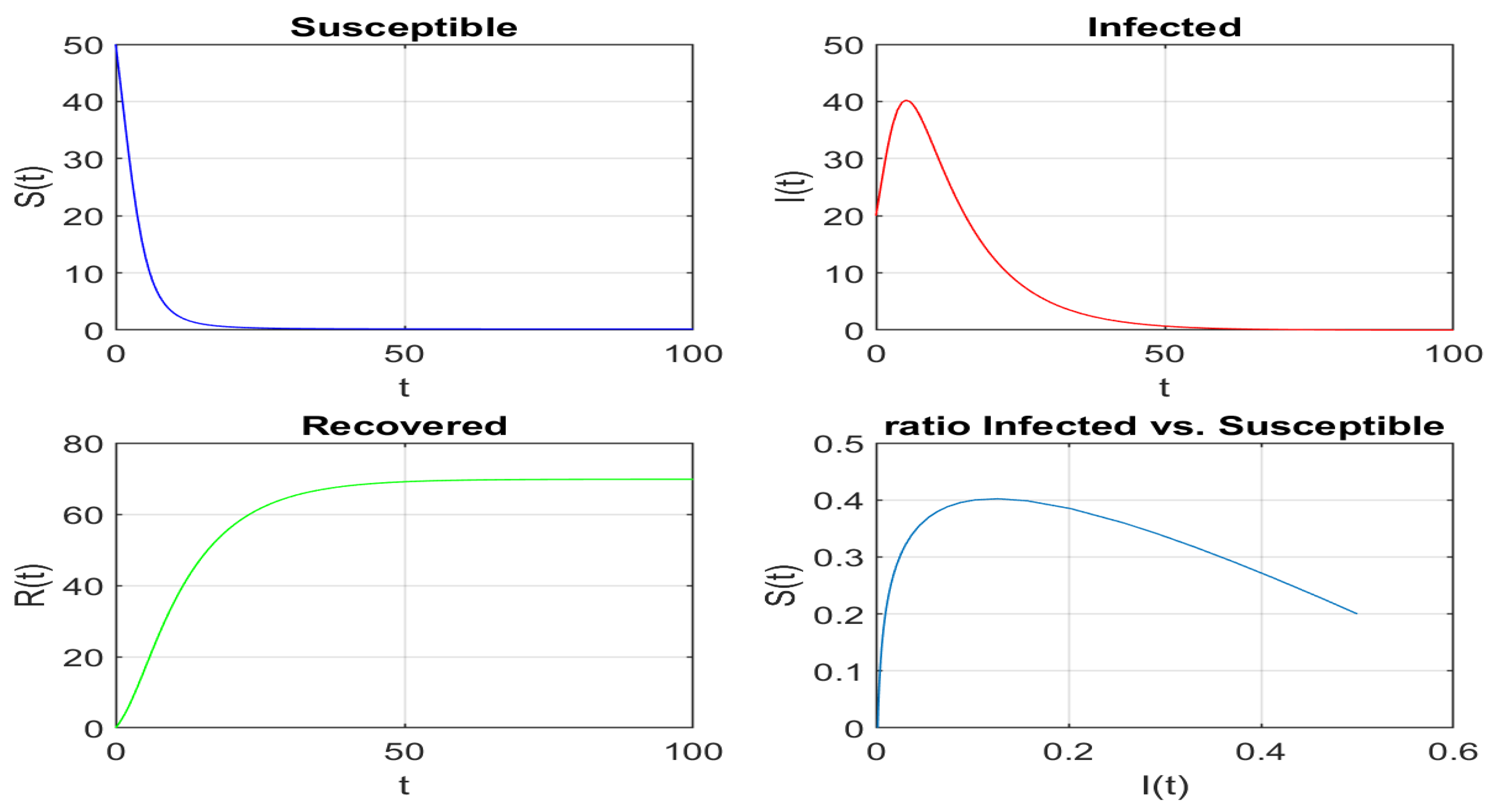
Formulation of the Fisrt Two Basic Epidemiology Models

The first epidemic model that I will describe is the classic SIR model that models diseases where some individuals start out being susceptible. These individuals can transition to a state of infection by contagion and after a time they transition to a state of recovery obtaining permanent immunity. The arrow labeled as horizontal incidence in Figure 1 represents the infection rate with which a susceptible individual is in contact with infected nodes and makes them transit to an infected state. S ( t ) represents the number of susceptible at time t, I ( t ) is the number of infected at time t, N the total size of the population, s ( t ) = S ( t ) N the fraction of susceptible of the total population at time t, i ( t ) = I ( t ) N the fraction of infected of the total population at time t, N the population size and β the average number of adequate contact or sufficient for transmission. The average number of contacts with infected per unit time of one susceptible is expressed as β I N = β i and β I N S = β N i s the number of new cases per unit time. The transitions from the boxes M , E and I in Figure 1 are calculated δ M , ϵ E and γ I . These terms represent the exponentially distributed waiting time in each box that in the cases of the I compartment in Figure 1 the transfer rate γ I P ( t ) = e γ t is the fraction that is still in the infective class t units after entering this class and 1 γ is the mean waiting time.
The parameters R 0 , σ and the replacement number R are related to the threshold. For more details about the classical SIR model consult the article [3].
After having defined the relevant elements of the phenomenon of the spread of a disease, we are able to define the following S I R epidemic model:
d S d t = β I S N , S ( 0 ) = S 0 0 d I d t = β I S N γ I , I ( 0 ) = I 0 0 d R d t = γ I , R ( 0 ) = R 0 0
where S ( t ) + I ( t ) + R ( t ) = N . If we divide by N (the total population) the Equation (1) we obtain
d s d t = β i s , s ( 0 ) = s 0 0 d i d t = β i s γ i , i ( 0 ) = i 0 0
with r ( t ) = 1 s ( t ) i ( t ) where s ( t ) , i ( t ) and r ( t ) are the fractions in the classes.
We are also able to define the following S I R endemic model
d S d t = μ N μ S β I S N , S ( 0 ) = S 0 0 d I d t = β I S N γ I μ I , I ( 0 ) = I 0 0 d R d t = γ I μ R , R ( 0 ) = R 0 0
where S ( t ) + I ( t ) + R ( t ) = N . The  S I R model (3) is almost the same as the epidemic version (1) except that it has an inflow of newborns into the susceptible class at rate μ N and deaths in the classes at rates μ S , μ I and μ R . If we divide by N (the total population) the Equation (3) we obtain
d s d t = β i s + μ μ s , s ( 0 ) = s 0 0 d i d t = β i s ( γ + μ ) i , i ( 0 ) = i 0 0
with r ( t ) = 1 s ( t ) i ( t ) where s ( t ) , i ( t ) and r ( t ) are the fractions in the classes.
For a deep exposition of more sophisticated models and analysis of their respective thresholds consult [3].
The next figure corresponds to a simulation of the SIR model.
In reference to Figure 2, as can be seen in the graphs generated by the simulation of the classical epidemic SIR model, the behavior in time of the infected curve reaches its peak or acme and then decreases until it is extinguished as expected since the type of epidemic processes that the model describes is related to infections that produce permanent immunity, which is also observed in the corresponding growth in behavior over time of the recovered curve. It is also important to note that the curve of the proportion of Infected vs. Susceptibles converges to a fixed point in the coordinates ( 0 , 0 ) , that is, the origin of said coordinate system. It is important to mention that in Figure 2  s ( ) > 0 even though it seems equal to zero.
The classical SIS model can be defined as follows
d S d t = β I S N + γ I , S ( 0 ) = S 0 0 d I d t = β I S N γ I , I ( 0 ) = I 0 0
The next figure corresponds to a simulation of the SIS model.
In reference to Figure 3, as can be seen in the graphs generated by the simulation of the classical epidemic SIS model, the number of infected decreases until it converges to some given level and simultaneously the number of susceptible grows until some level and stays there as expected, since the type of epidemic processes that the model describes is related to infections that produce temporary immunity. It is also important to note that the curve of the proportion of Infected vs. Susceptible converges to a fixed point in the coordinates ( 0.1 , 0.1 ) .

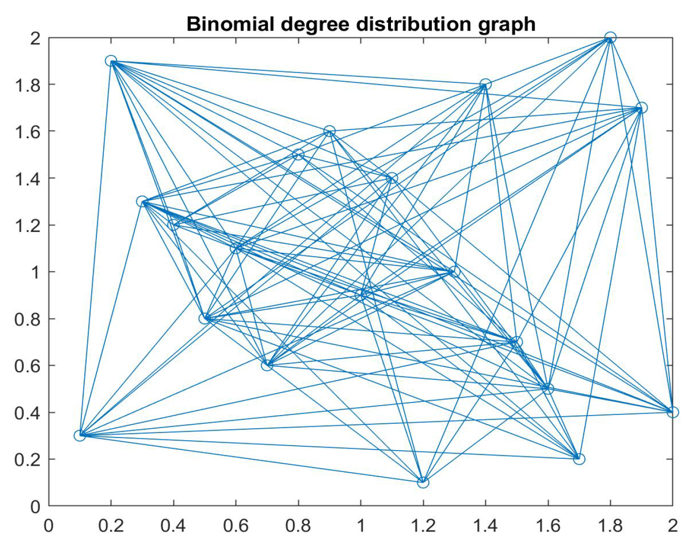
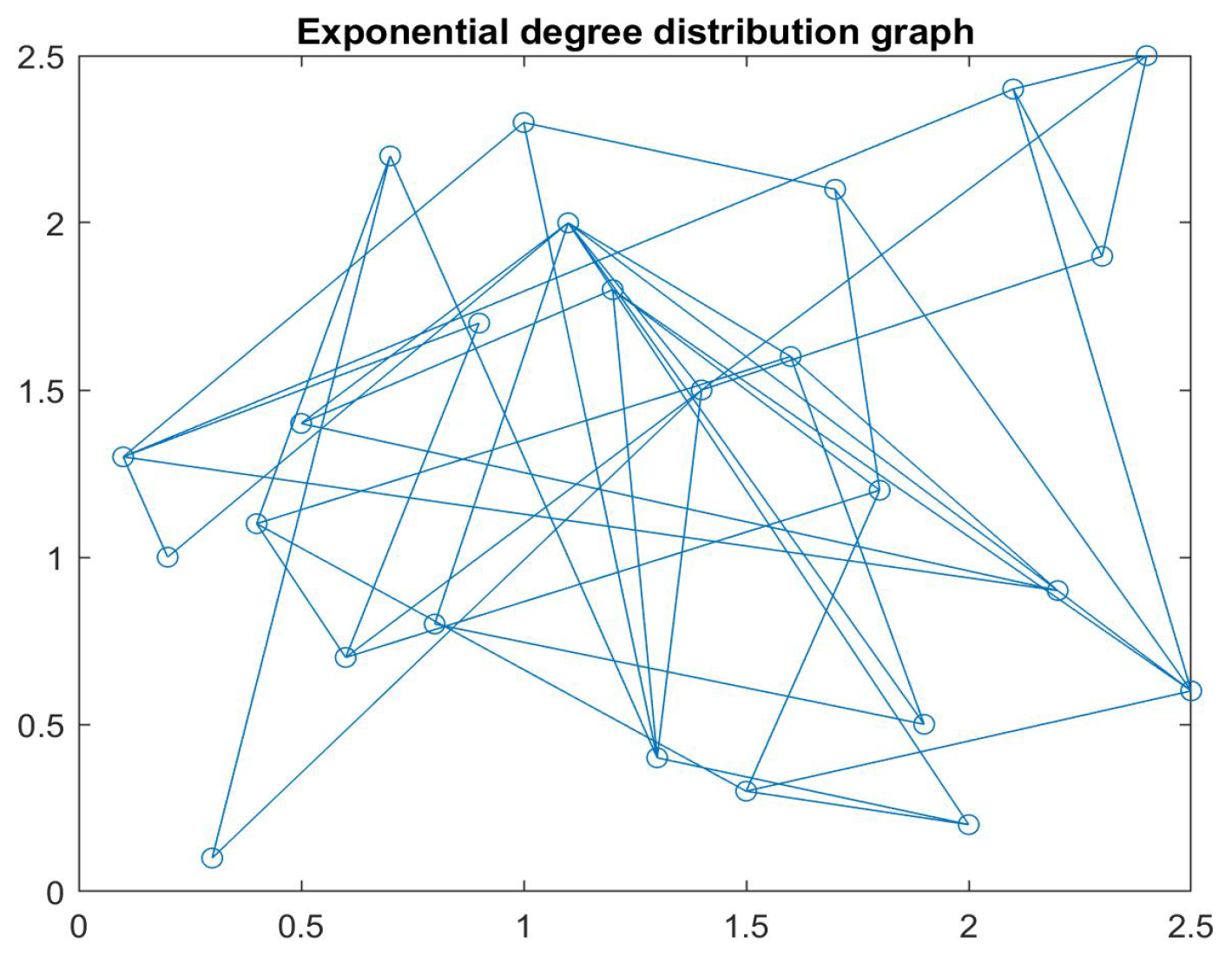
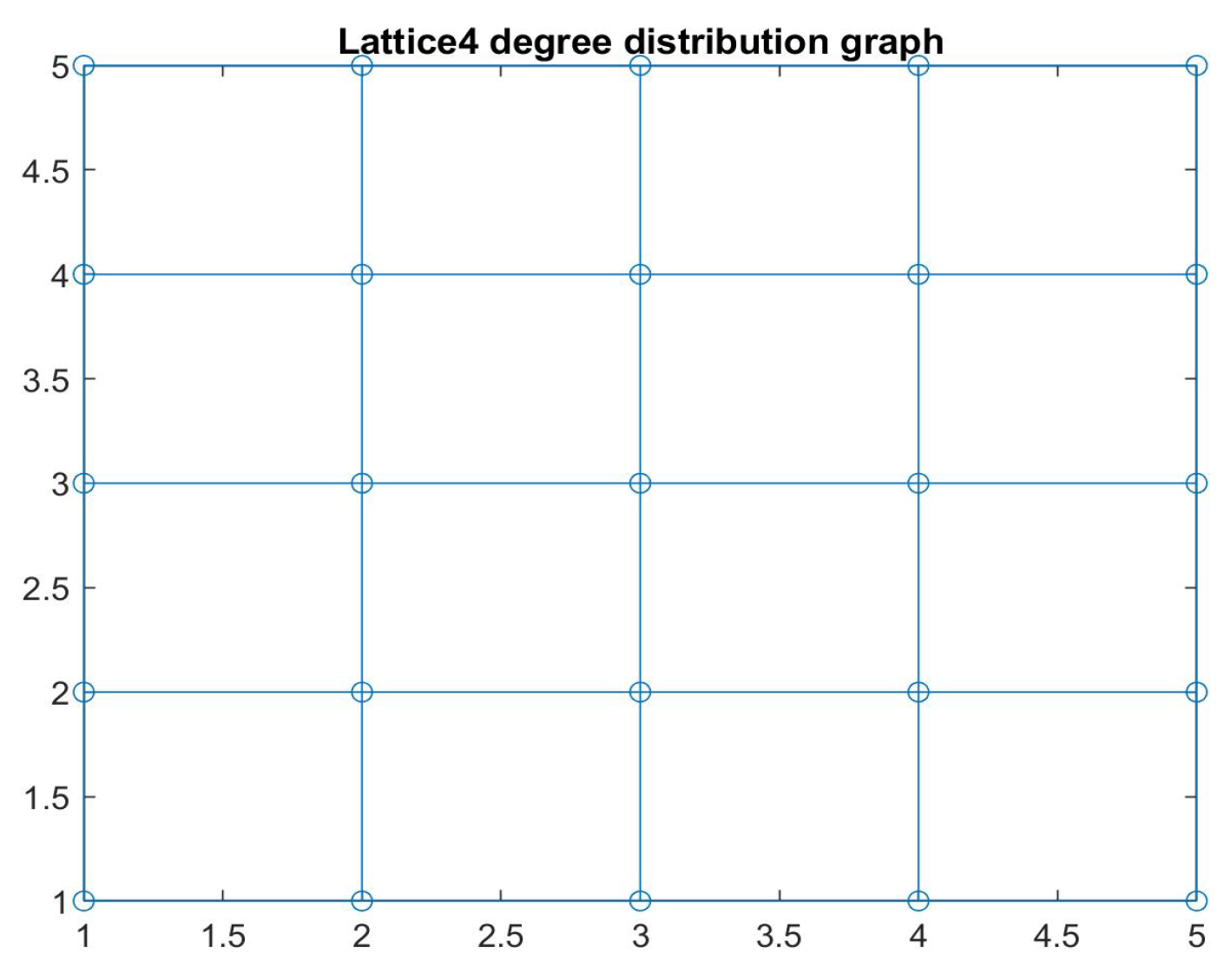
3. Discrete Epidemic Models in Networks

Mathematical epidemic models assume that each individual has on average the same number of contacts. In my opinion, this hypothesis is not always fulfilled because it does not correspond to the type of structures that arise in networks such as the internet in media such as Facebook or Twitter. In addition, the type of structures that appear in these social networks partly reflects the way in which people build networks of collaboration and interaction in real life. For this reason, I believe that just as the mathematical models of epidemics have contributed to the development of discrete mathematical models to study the phenomena of virus propagation in computer networks, also the mathematical models of epidemics can benefit from the advances that take place in the study of virus spread in computer networks. Since computer networks have grown rapidly, security problems have also increased in the same proportion. In the same way, the number of types of services offered on networks such as the Internet has grown. One service that appeared has been the distribution of content over the internet, which requires ensuring that the information reaches its destination quickly and with a good level of quality. In this type of service, P2P-type networks have been studied. Another type of service that arises with the appearance of networks is that of sensor networks. When trying to solve both security and quality of service problems, it is necessary to resort to mathematical tools that allow modeling the phenomena inherent in computer networks and answering questions such as which network structure is the most appropriate to ensure that the network stays connected in the presence of faults in the lines or what type of topology ensures that the distance traveled by an information packet is short enough for it to reach its destination without delays. On the other hand, the security of a network must be guaranteed, and therefore, it is important to know which network topology facilitates or inhibits the spread of a virus in it. These topics have aroused the interest of researchers from fields as varied as statistical physics or experts in the field of random graphs.
The type of graphs that appear most frequently in the study of virus propagation in complex networks and that we will use to illustrate the operation of discrete SIS models are those of binomial distribution of degrees, distribution of degrees in power laws, exponential type and lattices. For the sake of clarity, I give below the definitions of these types of graphs.
Definition 1.
Power law or scale-free degree distribution graph Is a graph whose degree distribution of nodes follows asymptotically a power law. More formally let P ( k ) be the fraction of the total number of nodes in a given graph that have k connections with other nodes. This fraction of nodes has the following behavior
P ( k ) k γ
where γ is a parameter in the interval 2 < γ < 3 .
Definition 2.
Binomial degree distribution graph (Erdős–Rényi model, Barabasi-Albert model, etc.) Is a random graph whose degree distribution of nodes follows a binomial probability distribution law of degrees k that can be formally defined as follows. Each of the n nodes of the graph is independently connected with another node with probability p or not connected with probability ( 1 p ) . Let P ( k ) be the fraction of the total number of nodes in a given graph that have k connections with other nodes. This fraction of nodes has the following behavior
P ( k ) = n 1 k p k ( 1 p ) n 1 k
Definition 3.
Exponential degree distribution graph  Is a random graph whose degree distribution of nodes follows a binomial probability distribution law of degrees k that can be formally defined as follows. Let P ( k ) be the fraction of the total number of nodes in a given graph that have k connections with other nodes. This fraction of nodes has the following behavior
P ( k , λ ) = λ e λ k k 0 0 k < 0
where  λ > 0  is a parameter of the distribution called rate parameter.
Definition 4.
Lattice 4 connected graph (grid graph, mesh graph, etc.)  Is a graph where each node is connected to four other nodes among all the n nodes belonging to the graph.
Next, I will show some examples of these graphs.
The understanding of the emergence of giant components or phenomena of small worlds that occur on the Internet requires mathematical tools such as the theory of contact processes as well as the theory of random graphs to be able to analyze these phenomena.
Many research articles have been written about such subjects [13,14,15,16,17,18,19]. Some papers about rumors spreading on networks under the approach of contact processes have also been written [20]. The problem of vaccine distribution on networks can be consulted in [21].
Figure 4, Figure 5, Figure 6 and Figure 7 are just some examples of network topologies that appear in the literature on complex networks and that account for the variety of degree distributions of the nodes that can be found in practice.
Finally the use of tools such as non-linear dynamical systems, and fix-point theorems for obtaining fast extinction conditions of a virus in a network combined with a discrete version of a SIS epidemic model can be found in [22]. This is the model that I will describe in the following subsection.

3.1. Discrete SIS and SIRS Epidemic Models

In order to understand the spread of viruses on a network, the model proposed in [22] assumes that the nodes behave according to a SIS-type model and that they are interconnected by a network. They also assume that we take very small discrete timesteps of size Δ t where Δ t 0 . The survivability results in [22] apply equally well to continuous systems. Within a Δ t time interval, each node i has probability r i of trying to broadcast its information every time step, and each link i j has a probability β i , j of being up, and thus correctly propagating the information to node j. Each node i also has a node failure probability δ i > 0 . Every dead node j has a rate γ j of returning to the up state, but without any information in its memory. Another important parameter of the Chakrabarti model is p i ( t ) which represents the probability that node i is alive at time t and has info, that is, the node is infected, q i ( t ) that represents the probability that node i is alive at time t and has no info, that is, the node is not infected and ζ i ( t ) that represents the probability that node i does not receive info from any of its neighbors at time t. The details about the parameters of this model as well as the fast extinction conditions and stability results can be consulted in [22]. the authors of [22] chose to use the non-linear dynamic systems approach and fixed point theorems. The state transitions at each node are shown in Figure 8.
The node state has info that can be thought of as being infected. The authors of [22] proposed to obtain an approximation of the threshold by describing the problem as a non-linear dynamic system with N variables representing the nodes and assumed that the state of two different nodes is independent. The independence condition can be formally expressed as follows:
ζ i ( t ) = j = 1 N ( 1 r j β j i p j ( t 1 ) )
Then equations describing the state transitions in the dynamic systems for each node, taking into account what is depicted in Figure 8, can be expressed as
p i ( t ) = p i ( t 1 ) ( 1 δ i ) + q i ( t 1 ) ( 1 ζ i ( t ) )
q i ( t ) = q i ( t 1 ) ( ζ i ( t ) δ i ) + ( 1 p i ( t 1 ) q i ( t 1 ) ) γ i
I include below the theoretical results related to the fast extinction condition without demonstration in order to have a clear description of the SIS model [23].
Definition 5.
Define S to be the N × N system matrix:
S i j = 1 δ i if i = j r j β j i γ i γ i + δ i o t h e r w i s e
Let | λ 1 , S | be the modulus of the largest eigenvalue and C ^ ( t ) = i = 1 N p i ( t ) the expected number of carriers at t of the dynamical system.
Theorem 1.
(Condition for fast extinction). Define s = | λ 1 , S | to be the  survivability score    for the system. If  s =   | λ 1 , S |   < 1 , then we have fast extinction in the dynamical system, that is, C ^ ( t ) decays exponentially quickly over time.
Two additional results that appears in [22] are the following:
Corollary 1.
(Condition for fast extinction homogeneous case for Chakrabati SIS model)  If δ i = δ , r i = r , γ i = γ , for all i, and  B = [ β i j ] is a symmetric binary matrix (links are undirected, and are always up or always down), then the condition for fast extinction is γ δ ( γ + δ ) λ 1 , B < 1 .
From the previous results Theorem 1 and Corollary 1 the fast extinction condition depends on the parameters δ , γ and β as well as on the largest eigenvalue λ 1 , S of the matrix of the dynamical system, and therefore, on the topology of the net.
Based on the Equations (10) and (11) of the SIS model, implement a simulation in MATLAB whose results I show below.
Figure 9 shows the behavior of the Chakrabarti SIS model in a power law-type network from five different initial conditions that consist of varying γ and β in increments of 0.05 . Each process converges to states where the number of infected is higher than the number of susceptible.
Figure 10 shows the behavior of the Chakrabarti under the same conditions as the behavior of the simulation in Figure 9 but the topology of the network is a lattice. It should be pointed out that the process in Figure 10 has some variations with respect to the one shown in Figure 9 due to the difference in the degree characteristics of the respective topologies.
Figure 11 shows the behavior of the Chakrabarti SIS model in a power law-type network from five different initial conditions that consist of varying γ in increments of 0.05 . Each process converges to states where the number of infected is higher than the number of susceptible.
Figure 12 shows the behavior of the Chakrabarti SIS model in a Lattice 4 type network from five different initial conditions that consist of varying γ in increments of 0.05 . It can be seen that the process achieves fast extinction conditions, or at least a significant reduction in the number of infected nodes, given that the topology is a lattice. So with this example, we can observe that the topology can make a difference between having a fast extinction of the epidemic or converging to a state where the number of infected is bigger than the number of susceptible and stays stable in such a state. In [24] it was formulated a similar discrete epidemic model proposed by the authors of [22] having one additional state in order to let the nodes be warned by a message or to receive a vaccine.
The idea behind this additional state was to explore prevention alternatives as well as the possible eradication of a virus in a computer network either through warning messages or by distribution of a vaccine [21]. The results regarding the fast extinction condition of the virus as well as the fixed point results were very similar to those of the [22] model. Each node can be in one of three states: Infected, Warn Info, No Info or Dead, with transitions between them as shown in Figure 13. The next graph represents the transitions that take place in each node for this model.
Making the same node independence probability assumption that is stated in Equation (9) and taking into account the new states and transition probabilities shown in Figure 13, the Equations (10) and (11) as well as the new equation corresponding to w i can be expressed as follows:
p i ( t ) = p i ( t 1 ) ( 1 δ i ) + q i ( t 1 ) ( 1 ζ i ( t ) ) ν i
q i ( t ) = q i ( t 1 ) ( ζ i ( t ) δ i ) + ( 1 p i ( t 1 ) q i ( t 1 ) w i ( t 1 ) ) γ i + χ i w i ( t 1 )
w i ( t ) = ( 1 ζ i ( t ) ) ( 1 ν i ) q i ( t 1 ) + ( 1 χ i δ i ) w i ( t 1 )
Based on the Equations (11), (12) and (14) of the SIRS model, I implemented a simulation in MATLAB whose results I show below.
Figure 14 shows the behavior of the SIRS model in a power law-type network from five different initial conditions that consist of varying γ and β in increments of 0.05 . Each process converges to states where the number of infected is higher than the number of susceptible.
From the behavior shown in Figure 14 and Figure 15 of the SIRS, we can claim that the topology has an impact on achieving the fast extinction of an epidemic model.
As we can see in the simulation graphs of this subsection, they were carried out with particular values of the parameters. In order to show that the Lattice-4 type topology has better behavior than the Powerlaw type topology, we will show below some simulations of the Chakrabarty SIS model for different values of the δ , γ and β parameters making increments of Δ = 0.05 in the three parameters simultaneously.
In the Figure 16, Figure 17, Figure 18, Figure 19, Figure 20, Figure 21, Figure 22 and Figure 23 it can be seen what the behavior of the Chakrabarti model is, both on the powerlaw type and lattice4 type network topology, by simultaneously varying its parameters. Finally, in order to show the behavior of the Chakrabarty SIS model, both in the Powerlaw type topology and in the Lattice4 type, varying a single parameter at a time, I will give some additional simulations. In the simulations that follow, only the parameter δ will be varied.
As can be seen in the Figure 24, Figure 25, Figure 26, Figure 27, Figure 28 and Figure 29, associated with the simulations where one of the parameters was varied at a time, the behavior relative to the rapid reduction in the number of infected of the Lattice4 type topology is significantly better than that of the Powerlaw type in each of the simulated cases.
In the simulations that follow, only the parameter γ will be varied.
In the simulations that follow, only the parameter β will be varied.

3.2. Time Complexity of the Simulations

It is important to know how much time is invested in the simulation process. To conduct this, a brief algorithmic analysis of the simulation must be made. First of all, we need to provide initial information such as the number of nodes, the number of time steps or time span of the simulation, the desired topology, and the values of the parameters of the epidemiological model. With this information, the adjacency matrix of the graph is generated. For each time step and for each node of the graph the mathematical expressions of the epidemiological model are evaluated. The simulation has the following algorithmic structure:
Ask for information: # of nodes n ,# of time steps t, parameters of  model
A=Generate_Adjacency_Matrix(n)
for i=1 to t
   for j=1 to n
      Evaluate_Model(i,n)
  end
end
  
Plot
Asking for input information instruction takes a constant number of steps. The generation of matrix A takes O ( n 2 ) steps. The evaluation of the model takes O ( t · n ) steps and given that t is a constant then the evaluation of the model is of order O ( n ) . Since this simulation iterates from 1 to 5 in order to increase the parameters with Δ then we must multiply the simulation time that I just outlined by the constant 5. Then the total time complexity of the simulation is T ( n ) = O ( n 2 ) .

4. Isolation Strategies

At the start of this section, it is worth carrying out a review of some articles that address the issue of the relationship between the efficiency with which a virus spreads in a network and its topological structure. In the article [25] it is explored the relationship between the epidemic threshold in a network and the spectrum of the graph adjacency matrix associated to the network. In the bibliography on virus propagation in networks consulted by the authors of [25], the existence of a critical epidemic threshold or phase change is mentioned, which they denote as τ c and that in the event that the ratio meets the inequality τ = β δ > τ c , where β represents the contagion rate and δ the healing rate of the node, the virus would persist and a non-zero fraction of nodes would remain infected, while if τ τ c , the epidemic would disappear. In the same article [25] the authors were motivated to understand the influence that structural characteristics of a graph have on the propagation process of a virus in a network. In their research, they found that the effective transmission threshold of the infection that they denoted as τ c is equal to 1 λ m a x ( A ) , where A represents the adjacency matrix of the graph associated with the network and λ m a x ( A ) is the largest eigenvalue of A. This eigenvalue is called the spectral radius of the network. These same authors mention that even in the case of applying approximate techniques such as the mean field theory, the epidemic threshold can be obtained in a well-defined way, in this case also being τ c = 1 λ m a x ( A ) .
In this same article, the authors review two epidemic models in order to understand the fine details of their N-interwined Markov chain model. These two basic models are the Kephart and White model and the Wang model. For reasons of clarity in the exposition, I will briefly describe these epidemic models below. The Kephart and White model considers a regular connected graph of N nodes where each node has degree k. The number of infected nodes at a time t will be denoted as I ( t ) and if the size N of the population is large enough we can define y ( t ) I ( t ) N representing the fraction of infected nodes. It is implicitly assumed that since the number of states is sufficiently large, the asymptotic regime for an infinite number of states is reached. The rate of change of y ( t ) is determined by two processes
  • Infected nodes are healing
  • Susceptible nodes are becoming infected
For the first process, the cure rate of a fraction y ( t ) of infected nodes is δ y and the rate of change of the growth of the fraction of infected nodes is proportional to the fraction of susceptible nodes, that is at 1 y . For each susceptible node, the infection rate is the product of the infection change rate β per link or neighbor, whose number is equal to k y . Taking the above into account we can establish the differential equation of said model, which would be the following
d y ( t ) d t = β k y ( 1 y ) δ y
whose solution is
y ( t ) = y 0 y y 0 + ( y y 0 ) exp ( β k δ ) t
where y 0 represents the initial fraction of infected nodes and y the fraction of infected in the steady-state assuming that d y d t = 0 . This model is the basis of a broader class of mean field models whose steady-state epidemic threshold is of the type
τ c = 1 k
Wang’s model is a generalization of Kephart and White’s that incorporates arbitrary networks characterized by their adjacency matrix A, whose only network characteristic is the average degree of the nodes. Wang’s model is also of the mean field class and its epidemic threshold is
τ c = 1 λ m a x ( A )
After that, they study the structure of the matrix of the infinitesimal generator Q of the exact N-interwined Markov chain model of 2 N states of a network of N nodes and give a precise result for the convergence time T on two specific graphs, which are the complete graph of N nodes and the linear graph of N nodes and compare it with the approximate mean field model from which they derive precise relationships as well as upper bounds for the steady-state to characterize the exponential decay τ < τ c , thus revealing the important role that plays the spectrum of the matrix A. Likewise, in order for the contribution of the authors of [25] to be clearer and better appreciated, I will make a brief description of their model of N-interwined Markov chains. The starting point in the definition of the exact Markov chain of 2 N states is a graph G ( N , L ) of N nodes and L edges on which a process of virus propagation is going to take place and whose adjacency matrix is A. The arrival of infections through a connection link between nodes as well as the healing process of a node are assumed to be independent Poisson processes with rates β and δ , respectively. Each node i when infected at a time t enters a state X i ( t ) = 1 and if it is not infected it is in a state X i ( t ) = 0 . At every moment each node is in one of these two states. The state of the network at time t denoted by Y ( t ) is defined by all possible combinations of states in which each of the N nodes can be found at time t
Y ( t ) = [ Y 0 ( t ) , Y 1 ( t ) , , Y 2 N 1 ( t ) ] T
and each Y i takes the following form
Y i ( t ) = 1 , i = k = 1 N X k ( t ) 2 k 1 0 , i k = 1 N X k ( t ) 2 k 1
Each state of the exact 2 N Markov chain diagram is labeled with an N position binary string where each bit x k { 0 , 1 } represents the state of each node in the network. The elements of the infinitesimal generator Q of the continuous-time Markov chain with 2 N states that define the virus infection process can be stated as follows
q i j = δ , i f i = j + 2 m 1 m = 1 , 2 , N ; x m = 1 β k = 1 N a m k x k i f i = j 2 m 1 m = 1 , 2 , N ; x m = 0 k = 1 ; k j q k j i f i = j 0 o t h e r w i s e
and each state is i = k N x k 2 k 1 . The probability time-dependent state vector s ( t ) has i components that can be expressed as follows
s i ( t ) = P r [ Y ( t ) = i ] = P r [ X 1 ( t ) = x 1 , X 2 ( t ) = x 2 , , X n ( t ) = x n ]
normalized in such a way that it meets the following condition
i = 0 2 N 1 s i ( t ) = 1
and obeys the following differential equation
d s T ( t ) d t = s ( t ) T Q
whose solution is
s T ( t ) = s T ( 0 ) exp Q t
Taking s i ( t ) as a joint probability distribution allows us to calculate the probability that a node j is in the state x j = 0 or x j = 1 adding as follows
P r [ X j ( t ) = x j ] = i = 0 , i j 2 N 1 s i ( t )
By defining v j ( t ) = P r [ X j ( t ) = 1 ] , the following relationship can be established between s ( t ) and v ( t )
v T ( t ) = s T ( t ) M
where M is a matrix of 2 N × N containing the states in binary with the bits in reverse order as follows
M = 0 0 0 0 1 0 0 0 0 1 0 0 1 1 0 0 0 0 1 0 1 1 1 1
The binary representation of the network allows us to obtain the structure of the matrix Q whose upper triangular matrix depends on the elements a i j of the matrix A and is, therefore, denoted as Q A , a lower triangular matrix Q δ that does not depend on A, with blocks B ( j ) = δ I 2 j × 2 j and a diagonal matrix Q d i a g whose elements are calculated as q j j = k = 1 , k j N q k j . This allows Q to be expressed as a sum of said matrices as Q = Q δ + Q A + Q d i a g . By analyzing the eigenstructure of Q and its spectral information they obtain bounds on the convergence times to the stable state of and calculate epidemic thresholds in terms of the largest eigenvalue on specific graphs such as the complete graph of N nodes K N as well as for the linear graph of N. This same spectral analysis of Q allows them to compare with the results obtained with the approximate mean field models of Kephart and White and of Wang. To do this, they perform simulations of the N-intertwined Markov chains and compare them with the results obtained with the exact Markov chain of 2 N states and realize that for all graphs, the N- interwined Markov chains approximate very well for the case τ < τ c . For the case of τ > τ c some differences in approximation arise which, however, tend to reduce as the number N of nodes in the network increases. Finally, the authors of [25] reach the conclusion that the topology of the networks must be taken into account in the processes of virus propagation in networks.

4.1. Previous Results in Isolation Strategies

In the context of epidemics, whether in people networks or computer networks, there are levels of isolation that range from completely isolating infected nodes to only reducing contacts in order to reduce as much as possible the speed of spread of an infectious virus. The complete isolation of nodes in a computer network can disconnect parts of a network until it is unable to function. In order to prevent this from happening, intermediate isolation strategies have been proposed in the last two decades by partially eliminating the contacts of an infected node, in such a way that the speed of spread of the virus is reduced as much as possible. The analysis of the spectrum of the adjacency matrix, that is to say, the set of eigenvalues of the said matrix, provides very valuable information about the structural characteristics of a graph. As mentioned above, the largest eigenvalue of the adjacency matrix λ 1 ( A ) is directly related to the critical transition threshold and this is expressed as τ c = 1 λ 1 ( A ) . One work related to the spectral analysis of the adjacency matrix that I found very revealing was that of [26]. In this article, the authors decrease the spectral radius by removing edges from the graph with the aim of minimizing it. Since said minimization is reducible to the search for a Hamiltonian path in a graph, then said minimization is NP-hard. The formal definition of the spectral radius optimization problem by means of graph edges provided in [26] is stated below.
Problem 1.
(Link Spectral Radius Minimization) or (LSRM) Given a graph  G ( N , L ) with N nodes and L links, spectral radius λ 1 ( G ) , and an integer number m < L , which m links from the graph G should be removed, such that the spectral radius of the reduced graph G m with L m links has the smallest spectral radius out of all possible graphs that can be obtained from G by removing m links?
After this, the authors of [25] state the following theorem.
Theorem 2.
The LSRM problem is NP-hard.
To prove the Theorem 2 the authors of said article resort to the following 3 lemmas that we enonce without proof.
Lemma 1.
The path P N 1 visiting N nodes has a strictly smaller spectral radius than all other connected graphs with N nodes Furthermore, λ 1 ( P N 1 ) = 2 cos ( π N + 1 ) .
The proof can be found in [27] page 125.
Lemma 2.
The eigenvalues of a disconnected graph are composed of the eigenvalues (including multiplicities) of its connected components.
The proof can be found in [27] pages 73–74.
Lemma 3.
Among all possible graphs of N nodes and N 1 links, the path P N 1 visiting N nodes has the smallest spectral radius.
The proof can be found in [25].
In order to prove the Theorem 2, the authors define the following problem.
Problem 2.
(Hamiltonian path problem). Given a graph G ( N , L ) with N nodes and L links, a Hamiltonian path is a path that visits every node exactly once. The Hamiltonian path problem is to determine if G contains a Hamiltonian path.
The authors of [25] prove the Theorem 2 by reduction of the Problem 1 to the Problem 2. The details of the proof can be found in [25].
For this reason the authors of [26] take on the task of proposing heuristic solutions to this problem by proposing several greedy strategies such as removing links l between node i and node j that is related to the product of the components ( x 1 ) i and ( x 1 ) j of the eigenvector x 1 associated to the largest eigenvalue of the adjacency matrix of the graph. These authors also demonstrate in [26] that their heuristic strategy is superior to any other in the vast majority of cases. Likewise, these authors deduce in this article a scaling law where they establish that the decrease in the spectral radius is inversely proportional to the number N of nodes.

4.2. My Node Isolation Strategy Proposal

As we could see in the simulations carried out in this article, I tested Chakrabarti’s SIS-type virus propagation models and an SIRS-type model published in [24] through simulations. These simulations were carried out on two topologies with very different structural characteristics in order to observe the impact of the graph structure on the virus propagation behavior in these networks. In fact, what I did was to submit, with the same epidemic model parameter values, two networks with the same number of nodes but one with dense topologies such as the Power-law type network and the other with a regular topology of degree 4 in the nodes. I named these regular topologies of degree 4 as Lattice4. What can be observed is that in the dense topologies, rapid extinction was not obtained while in the regular and sparse topology, rapid extinction was achieved. The topologies on which the simulations were carried out were the Powerlaw-type and the Lattice4-type. When carrying out the simulations in the two mentioned topologies I gave the same value to the parameters of the models to observe their behavior under the same circumstances. Additionally, I varied the epidemiological parameters in the same way in both topologies and I was able to observe the reduction in the spread of viruses in the Lattice4-type graph with respect to the Powerlaw-type graph. In the case of the Lattice4-type graph, a convergence to the state of rapid extinction of the virus was obtained. In The case of the Powerlaw-type topology their behavior under the same epidemic parameter settings, the contagion process converged to a state of generalized contagion of the nodes. It is worth mentioning that I have carried out these same simulations on other topologies and the comparative result between the Lattice4-type topology and the other topologies (Binomial-type and Exponential-type), is similar to the ones obtained with the Powerlaw-type network topology. An interesting spectral property of regular graphs is stated in the following theorem.
Theorem 3.
The maximum degree d m a x = m a x 1 j N d j is the largest eigenvalue of the adjacency matrix A of the connected graph G if and only if the corresponding graph is regular (i.e., d j = d m a x = r for al j).
The proof can be found in [27]. This result gives us an idea about the spectral radius of an approximately regular topology, that is, where almost all nodes have the same degree. In the case that the graph is approximately regular and not very dense, that is, the degree is small, then we can ensure that its spectral radius will also be small. As can be seen in the results obtained in the simulations of both the Chakrabarti SIS model and my SIRS model, the network topology has a significant impact on the rapid extinction of a computer virus in a network or its permanence in it. Given that the topology of the network is related to its adjacency matrix, a possible isolation strategy is to minimize the first eigenvalue of said matrix [26]. The question is that this strategy would be reduced to the search for a Hamiltonian path, which in general is an NP-hard problem. One possibility is to look for algorithms that approximate the minimum value Hamiltonian path by algorithmic with some approximation guarantee and eliminate from the original interconnection graph those edges that do not belong to the just mentioned path. This is what is proposed in [26].
Taking into account the Theorem 3 and given the rapid extinction properties of the Lattice4-type topology, I am able to propose a link remotion node isolation strategy that allows me to reduce the spectral radius of a dense graph like the Powerlaw-type and even other less dense topologies, as an alternative to the node isolation strategies proposed in [25]. My node isolation strategy can be seen as a process of regularization of a dense graph that transforms it into an approximately regular topology where the degrees of the nodes are small and close to the value of 4. The semi-regularization transformation strategy of the original dense graph would do the following. First I would make a copy of the adjacency matrix of the original graph to make the modifications to the copy. It would go through each row of the copy of the adjacency matrix to keep a record of the degrees of each node in a vector. Afterwards, it would scan the adjacency matrix of the copy to detect a value of 1 in row i and column j if there is an edge between those nodes. If so, I would delete this edge by putting a 0 in the position A ( i , j ) as well as in the position A ( j , i ) of the adjacency matrix of the copy and would be discounted from the respective records of the degrees of the nodes involved in the removal of the edge, that are recorded in the mentioned vector, until reaching the value of 4 that represents the desired node degree. In order to make the description of my node isolation strategy clearer, below I make a description of it in algorithmic format.
Transform(A,B)
Copy(B,A);
r=rows(B);
c=columns(B);
for i=1:r
  d(i)=0;  // initialize de degree counter of node i
  for j=1:c
   d(i)=d(i)+B(i,j);
  end
  // start of edge removal for the regularization of the Powerlaw-type graph
  for k=1:c
   if (d(i)>=4) && (d(k)>=4)
    if B(i,k) == 1
     B(i,k)=0;
     d(i)=d(i)-1;
     B(k,i)=0;
     d(k)=d(k)-1;
    end
   end
  end
end
I implemented this procedure in MATLAB and tested it with a 20 node Powerlaw-type graph and the graphs involved in such transformation are shown in the Figure 30.
An application to contain the spread of a virus in a network, be it computerized or of people, could be to detect the value of the parameters that characterize a process of diffusion of a virus taking into account the interconnection medium where the epidemic process will take place and from there determine which network nodes to isolate by modifying the adjacencies of the associated graph in such a way as to obtain a notable reduction in the spread of a virus or even achieve its rapid extinction.
The graphs involved in the same transformation tested with a 50 node Powerlaw-type graph are shown in Figure 31.
In order to illustrate the positive impact of the proposed node isolation strategy, I will simulate Chakrabarti’s SIS epidemiological model on a Powerlaw topology and then apply the transformation of this topology and run the same Chakrabarti’s SIS epidemiological model on the modified topology. We first show the simulation of Chakrabarti’s SIS-type epidemiological model on a Powerlaw-type network on a network of n = 100 nodes.
In the Figure 32 shows the simulation of Chakrabarti’s SIS-type epidemiological model on the approximately regular 4 degree topology obtained after applying the proposed node isolation strategy over the Powerlaw-type network of the Figure 33.
In order to complete the test of the proposed node isolation strategy, I will apply the simulations of my SIRS model to a Powerlaw network and also to the topology transformed with my isolation strategy.
We first show the simulation of my SIRS-type epidemiological model on a Powerlaw-type network on a network of n = 100 nodes.
Figure 32 shows the simulation of my SIRS-type epidemiological model on the approximately regular 4 degree topology obtained after applying the proposed node isolation strategy over the Powerlaw-type network of the Figure 34.
From the simulations shown in Figure 32, Figure 33, Figure 34 and Figure 35, we can notice that the transformation obtained with the isolation strategy that I am proposing induces the rapid extinction of the epidemic.

5. Conclusions and Future Work

In this article, I make a historical account of the classical mathematical models for the study of epidemic processes that made it possible to develop models to address problems of virus spread in networks. In the previous sections, I showed by means of simulations, that the regular topologies whose degrees in the nodes are small, that is to say of degree 4, as is the case of the Lattice-4 topology, have a fast extinction property. This implies that virus propagation performance is better in the Lattice4-type topology than in other denser and less regular topologies as are the topologies of binomial type as well as those of Power law type. This allowed me to elaborate on a computationally efficient node isolation strategy that transforms an initially dense and irregular graph into an average regular graph that induces fast virus extinction in a network even though it is not optimal in the sense of the spectral radius. The isolation strategy that I propose in the present article, is an alternative to the heuristic strategies proposed in [26] to deal with the complexity of the problem mentioned in that article. In the article [26] heuristic node isolation strategies are presented that seek to minimize the associated spectral radius of a graph either by eliminating edges or by eliminating nodes. Because obtaining the optimum is reducible to the search for a Hamiltonian path in the graph and this is an NP-hard problem, they resort to the use of heuristic greedy algorithms and empirically determine the best one. In that sense, the authors of [26] obtain approximations to the optimum using heuristics that may not work in some cases. My strategy is more systematic and avoids the use of heuristics. Additionally, the node isolation strategy that I propose has the advantage of being computationally efficient and although it is not an optimal strategy, it induces the property of fast extinction of virus propagation in the network. As mentioned at the beginning of the Section 1, the nature of this article is theoretical. However, we can imagine applications in practice. One possible future application would be to use the proposed node isolation strategy to reduce the number of infections when no vaccine is available to deal with a deadly virus. Let us take as an example the case of the beginning of the COVID-19 pandemic. There were no vaccines and there was no knowledge of its mode of transmission or its lethality. Under these circumstances, the strategy initially proposed was radical isolation to prevent the spread of an unknown virus. This strategy caused social, psychological and economic problems in the population. A less radical alternative strategy could be one of the types proposed in this article. Along the present article, we were also able to observe that the concerns that arise in the field of virus spread on networks can contribute ideas to the development of mathematical models in epidemiology by incorporating aspects of the interconnection networks on which epidemics take place. By introducing the structures of interconnection networks to epidemiological models, we can obtain elements that guide epidemiologists in making decisions about isolation strategies to try to contain and eventually eradicate disease through the development of strategies based on knowledge of the dissemination of information in interconnection networks.

Funding

This research received no external funding.

Data Availability Statement

No new data were created or analyzed in this study. Data sharing is not applicable to this article.

Acknowledgments

This work was sponsored by the Department of Information Technologies, Universidad Autónoma Metropolitana Unidad Cuajimalpa, México.

Conflicts of Interest

The author declares no conflicts of interest.

Abbreviations

The following abbreviations are used in this manuscript:
SIR modelSusceptible, Infected and Recovered model
SIS modelSusceptible, Infected and Susceptible model
SIRS modelSusceptible, Infected, Recovered and Susceptible model
LSRMLink Spectral Radius Minimization

References

  1. Prakash, B.A.; Chakrabarti, D.; Faloutsos, M.; Valler, N.; Faloutsos, C. Got the Flu (or Mumps)? Check the Eigenvalue! arXiv 2010, arXiv:1004.0060. [Google Scholar]
  2. Chakrabarti, D.; Wang, Y.; Wang, C.; Leskovec, J.; Faloutsos, C. Epidemic Thresholds in Real Networks. Acm Trans. Inf. Syst. Secur. 2008, 10, 13. [Google Scholar] [CrossRef]
  3. Hethcote, H.W. The Mathematics of Infectious Diseases. Siam Rev. 2000, 42, 599–653. [Google Scholar] [CrossRef]
  4. Durrett, R. Random Graph Dynamics; Cambridge Series in Statistical and Probabilistic Mathematics; Cambridge University Press: Cambridge, UK, 2007. [Google Scholar]
  5. Bernoulli, D. Esai d’une nouvelle analyse de la mortalité causeé par la petite vérole et des avantages de l’inoculation pour la prévenir. In Memoires de Mathématiques et de Physique; Académie Royale des Sciences: Paris, France, 1760; pp. 1–45. [Google Scholar]
  6. Hamer, W.H. Epidemic disease in England. Lancet 1906, 1, 733–739. [Google Scholar]
  7. Ross, R. The Prevention of Malaria, 2nd ed.; Murray: London, UK, 1911. [Google Scholar]
  8. Bailey, N.T.J. The Mathematical Theory of Infectious Diseases, 2nd ed.; Hafner: New York, NY, USA, 1975. [Google Scholar]
  9. Dietz, K. Epidemics and rumours: A survey. J. R. Stat. Soc. Ser. A 1967, 130, 505–528. [Google Scholar] [CrossRef]
  10. Dietz, K. The first epidemic model: A historical note on P. D. En’ko. Austral. J. Stat. 1988, 30, 56–65. [Google Scholar] [CrossRef]
  11. Kermack, W.O.; McKendrick, A.G. Contributions to the mathematical theory of epidemics part 1. Proc. R. Soc. Lond. Ser. A 1927, 115, 700–721. [Google Scholar]
  12. McKendrick, A.G. Applications of mathematics to medical problems. Proc. Edinb. Math. Soc. 1926, 44, 98–130. [Google Scholar] [CrossRef]
  13. Durrett, R.; Liu, X.-F. The contact process on a finite set. Ann. Probab. 1988, 16, 1158–1173. [Google Scholar] [CrossRef]
  14. Albert, R.; Barabási, A.L.; Jeong, H. Error and attack tolerance of complex networks. Nature 2000, 406, 378–382. [Google Scholar] [CrossRef] [PubMed]
  15. Barabási, A.L.; Albert, R. Emergence of scaling in random graphs. Science 1999, 286, 509–512. [Google Scholar] [CrossRef]
  16. Ben-Avraham, D.; Barabási, A.L.; Schwartz, N.; Cohen, R.; Havlin, S. Percolation in directed scale-free networks. Phys. Rev. E 2002, 66, 0151041–0151044. [Google Scholar]
  17. Pastor-Satorras, R.; Vespignani, A. Epidemic dynamics and endemic states in complex networks. Phys. Rev. E 2001, 63, 0661171–0661178. [Google Scholar] [CrossRef] [PubMed]
  18. Pastor-Satorras, R.; Vespignani, A. Epidemic spreading in scale-free networks. Phys. Rev. Lett. 2001, 86, 3200–3203. [Google Scholar] [CrossRef]
  19. Pastor-Satorras, R.; Vespignani, A. Epidemic dynamics in finite size scale-free networks. Phys. Rev. E 2002, 65, 0351081–0351084. [Google Scholar] [CrossRef] [PubMed]
  20. Kempe, D.; Kleinberg, J. Protocols and impossibility results for gossip-based communication mechanisms. In Proceedings of the Symposium on Foundations of Computer Science (FOCS 2002), Vancouver, BC, Canada, 19 November 2002. [Google Scholar]
  21. Borgs, C.; Chayes, J.; Ganesh, A.; Saberi, A. How to distribute antidote to control epidemics. Random Struct. Algorithms 2010, 37, 204–222. [Google Scholar] [CrossRef]
  22. Faloutsos, C.; Madden, S.; Guestrin, C.; Leskovec, J.; Chakrabarti, D.; Faloutsos, M. Information survival threshold in sensor and p2p networks. In Proceedings of the IEEE INFOCOM 2007, Anchorage, AK, USA, 6–12 May 2007. [Google Scholar]
  23. Krivelevich, M.; Sudakov, B. The largest eigenvalue of sparse random graphs. arXiv 2001, arXiv:math/0106066v1. [Google Scholar] [CrossRef]
  24. Rodríguez Lucatero, C.; Bernal Jaquez, R. Virus and Warning Spread in Dynamical Networks. Adv. Complex Syst. 2011, 14, 341–358. [Google Scholar] [CrossRef]
  25. Van Mieghem, P.; Omic, J.; Kooij, R. Virus Spread in Networks. IEEE/Acm Trans. Netw. 2009, 7, 1–14. [Google Scholar] [CrossRef]
  26. Van Mieghem, P.; Stevanovi’c, D.; Kuipers, F.; Li, C.; van de Bovenkamp, R.; Liu, D.; Wang, H. Decreasing the spectral radius of a graph by link removals. Phys. Rev. 2011, 84, 016101. [Google Scholar] [CrossRef] [PubMed]
  27. Van Mieghem, P. Graph Spectra for Complex Networks; Cambridge University Press: Cambridge, UK, 2010. [Google Scholar]
Figure 1. The general transfer diagram for the MSEIR model.
Axioms 13 00079 g001
Figure 2. Simulation of classical epidemic SIR model with β = 0.8 , γ = 0.1 .
Axioms 13 00079 g002
Figure 3. Simulation of classical epidemic SIS model with β = 1 , γ = 0.1 .
Axioms 13 00079 g003
Figure 4. Binomial degree distribution graph.
Axioms 13 00079 g004
Figure 5. Exponential degree distribution graph.
Axioms 13 00079 g005
Figure 6. Power law degree distribution graph.
Axioms 13 00079 g006
Figure 7. Lattice 4 graph.
Axioms 13 00079 g007
Figure 8. Chakrabarti SIS model.
Axioms 13 00079 g008
Figure 9. Simulation of Chakrabarti SIS model with δ = 0.1 , γ = 0.1 + Δ , β = 0.1 + Δ on a Power law network. Each color in the graph p ( t ) vs. q ( t ) corresponds to the different values of the incremented parameters.
Axioms 13 00079 g009
Figure 10. Simulation of Chakrabarti SIS model with δ = 0.1 , γ = 0.1 + Δ , β = 0.1 + Δ on a Lattice 4 network. Each color in the graph p ( t ) vs. q ( t ) corresponds to the different values of the incremented parameters.
Axioms 13 00079 g010
Figure 11. Simulation of Chakrabarti SIS model with δ = 0.5 + Δ , γ = 0.3 , β = 0.4 on a Power law network. Each color in the graph p ( t ) vs. q ( t ) corresponds to the different values of the incremented parameters.
Axioms 13 00079 g011
Figure 12. Simulation of Chakrabarti SIS model with δ = 0.5 + Δ , γ = 0.3 , β = 0.4 on a Lattice 4 network. Each color in the graph p ( t ) vs. q ( t ) corresponds to the different values of the incremented parameters.
Axioms 13 00079 g012
Figure 13. The SIRS model.
Axioms 13 00079 g013
Figure 14. Simulation of SIRS model with δ = 0.6 , γ = 0.6 + Δ , ν = 1 , χ = 1 , β = 0.3 on a Power law network. Each color in the graph p ( t ) vs. q ( t ) corresponds to the different values of the incremented parameters.
Axioms 13 00079 g014
Figure 15. Simulation of SIRS model with δ = 0.6 , γ = 0.6 + Δ , ν = 1 , χ = 1 , β = 0.3 on a Lattice 4 network. Each color in the graph p ( t ) vs. q ( t ) corresponds to the different values of the incremented parameters.
Axioms 13 00079 g015
Figure 16. Simulation of Chakrabarti SIS model with δ = 0.1 + Δ , γ = 0.3 + Δ , β = 0.4 + Δ on a Powerlaw network. Each color in the graph p ( t ) vs. q ( t ) corresponds to the different values of the incremented parameters.
Axioms 13 00079 g016
Figure 17. Simulation of Chakrabarti SIS model with δ = 0.1 + Δ , γ = 0.3 + Δ , β = 0.4 + Δ on a Lattice-4 network. Each color in the graph p ( t ) vs. q ( t ) corresponds to the different values of the incremented parameters.
Axioms 13 00079 g017
Figure 18. Simulation of Chakrabarti SIS model with δ = 0.7 + Δ , γ = 0.3 + Δ , β = 0.4 + Δ on a Powerlaw network. Each color in the graph p ( t ) vs. q ( t ) corresponds to the different values of the incremented parameters.
Axioms 13 00079 g018
Figure 19. Simulation of Chakrabarti SIS model with δ = 0.7 + Δ , γ = 0.3 + Δ , β = 0.4 + Δ on a Lattice-4 network. Each color in the graph p ( t ) vs. q ( t ) corresponds to the different values of the incremented parameters.
Axioms 13 00079 g019
Figure 20. Simulation of Chakrabarti SIS model with δ = 0.7 + Δ , γ = 0.5 + Δ , β = 0.4 + Δ on a Powerlaw network. Each color in the graph p ( t ) vs. q ( t ) corresponds to the different values of the incremented parameters.
Axioms 13 00079 g020
Figure 21. Simulation of Chakrabarti SIS model with δ = 0.7 + Δ , γ = 0.5 + Δ , β = 0.4 + Δ on a Lattice-4 network. Each color in the graph p ( t ) vs. q ( t ) corresponds to the different values of the incremented parameters.
Axioms 13 00079 g021
Figure 22. Simulation of Chakrabarti SIS model with δ = 0.7 + Δ , γ = 0.5 + Δ , β = 0.3 + Δ on a Powerlaw network. Each color in the graph p ( t ) vs. q ( t ) corresponds to the different values of the incremented parameters.
Axioms 13 00079 g022
Figure 23. Simulation of Chakrabarti SIS model with δ = 0.7 + Δ , γ = 0.5 + Δ , β = 0.3 + Δ on a Lattice-4 network. Each color in the graph p ( t ) vs. q ( t ) corresponds to the different values of the incremented parameters.
Axioms 13 00079 g023
Figure 24. Simulation of Chakrabarti SIS model with δ = 0.5 + Δ , γ = 0.5 , β = 0.3 on a Powerlaw network. Each color in the graph p ( t ) vs. q ( t ) corresponds to the different values of the incremented parameters.
Axioms 13 00079 g024
Figure 25. Simulation of Chakrabarti SIS model with δ = 0.5 + Δ , γ = 0.5 , β = 0.3 on a Lattice4 network. Each color in the graph p ( t ) vs. q ( t ) corresponds to the different values of the incremented parameters.
Axioms 13 00079 g025
Figure 26. Simulation of Chakrabarti SIS model with δ = 0.5 , γ = 0.5 + Δ , β = 0.3 on a Powerlaw network. Each color in the graph p ( t ) vs. q ( t ) corresponds to the different values of the incremented parameters.
Axioms 13 00079 g026
Figure 27. Simulation of Chakrabarti SIS model with δ = 0.5 , γ = 0.5 + Δ , β = 0.3 on a Lattice4 network. Each color in the graph p ( t ) vs. q ( t ) corresponds to the different values of the incremented parameters.
Axioms 13 00079 g027
Figure 28. Simulation of Chakrabarti SIS model with δ = 0.5 , γ = 0.5 , β = 0.3 + Δ on a Powerlaw network. Each color in the graph p ( t ) vs. q ( t ) corresponds to the different values of the incremented parameters.
Axioms 13 00079 g028
Figure 29. Simulation of Chakrabarti SIS model with δ = 0.5 , γ = 0.5 , β = 0.3 + Δ on a Lattice4 network. Each color in the graph p ( t ) vs. q ( t ) corresponds to the different values of the incremented parameters.
Axioms 13 00079 g029
Figure 30. The transformation of a Powerlaw topology of n = 20 to a almost regular d = 4 topology of n = 20 nodes.
Axioms 13 00079 g030
Figure 31. The transformation of a Powerlaw topology of n = 50 to an almost regular d = 4 topology of n = 50 nodes.
Axioms 13 00079 g031
Figure 32. Simulation of Chakrabarti SIS model with δ = 0.5 + Δ , γ = 0.3 , β = 0.4 on the transformed almost regular network. Each color in the graph p ( t ) vs. q ( t ) corresponds to the different values of the incremented parameters.
Axioms 13 00079 g032
Figure 33. Simulation of Chakrabarti SIS model with δ = 0.5 + Δ , γ = 0.3 , β = 0.4 on a Power law network. Each color in the graph p ( t ) vs. q ( t ) corresponds to the different values of the incremented parameters.
Axioms 13 00079 g033
Figure 34. Simulation of my SIRS model with δ = 0.6 , γ = 0.6 + Δ , ν = 1 , χ = 1 , β = 0.3 on a Power law network. Each color in the graph p ( t ) vs. q ( t ) corresponds to the different values of the incremented parameters.
Axioms 13 00079 g034
Figure 35. Simulation of my SIRS model with δ = 0.6 , γ = 0.6 + Δ , ν = 1 , χ = 1 , β = 0.3 on the transformed almost regular network. Each color in the graph p ( t ) vs. q ( t ) corresponds to the different values of the incremented parameters.
Axioms 13 00079 g035
Disclaimer/Publisher’s Note: The statements, opinions and data contained in all publications are solely those of the individual author(s) and contributor(s) and not of MDPI and/or the editor(s). MDPI and/or the editor(s) disclaim responsibility for any injury to people or property resulting from any ideas, methods, instructions or products referred to in the content.

