Abstract
In this paper, the robustness of a system with sundry disturbed open loop dynamics is investigated by employing robust right coprime factorization (RRCF). These sundry disturbed open loop dynamics are present not only in the feed forward path, but also within the feedback loop. In such a control framework, the nominal plant is firstly right coprime factorized and a feed forward and a feedback controllers are designed based on Bezout identity to ensure the overall stability. Subsequently, considering the sundry disturbed open loop dynamics, a new condition formulated as a disturbed Bezout identity is put forward to achieve the closed loop stability of the system, even in the presence of disturbances existing in sundry open loops, where in the feedback loop a disturbed identity operator is defined. This approach guarantees the system robustness if a specific inequality condition is satisfied. And, it should be noted that the proposed approach is applicable to both linear and nonlinear systems with sundry disturbed open loop dynamics. Simulations demonstrate the effectiveness of our methodology.
Keywords:
robust stability; sundry disturbed open loop dynamics; Bezout identity; disturbed identity operator MSC:
93-XX; 80-XX; 47-XX
1. Introduction
In all practical processes that are often mathematically nonlinear, disturbed open loop dynamics, generally in the form of perturbation, disturbances, uncertainties, and so on, exist as inevitable phenomenons. Such open loop dynamics result from parameter variation, unmodeled dynamics, time delay, noise and other interference factors, and may locate in sundry units of the system. It has the potential of causing performance degradation, and even makes a stable open loop system an unstable one, thus it is essential to take into account these disturbed open loop dynamics when performing controlling for a plant.
Stochastic control [1,2] and robust control [3,4], as integral components of modern control theory, inherently possess the capability to address anti-disturbed open loop dynamics. The various disturbed open loop dynamics taking the form of unknown external disturbances [5], periodic disturbances of unknown frequency [6], plant uncertainties and input disturbances [7], unknown distributed disturbances [8], aleatory uncertainty involving random noises [9], uncertainty with objectives and constraints in terms of dynamic coherent risk measures [10], uncertainties in both the regressor matrix and parameter vector [11], structured linear time-varying model uncertainty [12], uncertain inputs and bounded variation [13], model uncertainty [14], unknown-but-bounded noises [15], unmeasurable disturbances [16], and bounded measurement noises [17] have been investigated. Sliding mode control is a highly effective nonlinear control approach, since it remains invariant to disturbed open loop dynamics [18,19,20,21,22,23].
Furthermore, robust right coprime factorization (RRCF) [24,25,26], where a plant is represented as a mapping from the input space to the output space, enabling control design in the time domain, has been explored for systems with disturbed open loop dynamics. It possesses the benefits of facilitating straightforward analysis for robust stability under disturbed open loop dynamics and being extendable to the control for multi-input multi-output systems, and has been successfully implemented across various control applications. Ref. [27] focuses on robust passive tracking control for an uncertain soft actuator using RRCF. In [28], a robust parallel compensator is utilized, ensuring the availability of a constant gain output feedback controller for plants with disturbed open loop dynamics in the form of structured uncertainty. In [29], time-varying multi-joint human arm viscoelasticity is estimated in real time, where the disturbed open loop dynamics taking the form of time-varying motor commands, measurement noises and modeling errors of the rigid body dynamics are taken into account. Ref. [30] overcomes the influence of disturbed open loop dynamics in the form of external disturbances, by combining the passivity-based control and RRCF, for the double inverted pendulum system. In [31], robust stability and tracking performance of a class of nonlinear systems with disturbed open loop dynamics in the form of external disturbance and internal perturbation are addressed by RRCF. Ref. [32] leverages RRCF for the robust nonlinear control of wireless power transfer systems, where the disturbed open loop dynamics due to the inaccurate distance between the transmit coil and receive coil, as well as variations in the output load are considered.
In this paper, sundry disturbed open loop dynamics attenuation or rejection problems are investigated by applying RRCF approach. Sundry disturbed open loop dynamics manifest in the forward and feedback loop, which is caused by the prevalent uncertainties and disturbances in the forward path coupled with the frequent occurrence of time delays and sensor noise in the feedback loop. In the proposed approach, firstly, the plant is right coprime factorized, and two controllers in the forward and feedback paths are designed based on a Bezout identity to ensure bounded input bounded output (BIBO) stability. For disturbed open loop dynamics in the forward path that result from uncertainties or noise, which is imposed on the plant input, two controllers designed satisfying a condition structured as an inequality guarantees the robust stability of the system. This is a conventionally employed method in robust right coprime factorization approach for perturbed plants, where the robust stability is achieved against disturbed dynamics in forward open loop. Additionally, it should be noted that the robust stability is ensured built upon the assumption that the mapping from plant output to the feedback controller input is an identity. A non-identity mapping of (plant) output-to-input (of feedback controller) cannot necessarily guarantee the above robust stability when there exist backward disturbed open loop dynamics. A filter approach is an appropriate option for dealing with such backward disturbed open loop dynamics which can avoid the redesign of controllers. In this work, disturbed open loop dynamics in the feedback path generated from unknown time-varying delay and noise which cause a non-identity in the mapping of output-to-controller is considered. The adverse effect due to the disturbed open loop dynamics is alleviated by adopting a filter variant. However, it is to be remarked that even the use of filter approach would not always enable the output-to-controller an identity. That is, even if some part of the disturbed dynamics has been mitigated, some residual perturbed ones may continue to impact system performance which renders the above mentioned robust stability conditions no longer applicable. Thus, a disturbed Bezout identity in a new form is formulated where a disturbed identity is adopted for notation of the effect of insufficient filter compensation for delay and noise. In one word, for sundry disturbed open loop dynamics, a new robust right coprime factorization scheme is proposed where the robust stability is guaranteed by a condition in a new inequality different from previous one. By using such a control framework, the overall stability can be confirmed in the presence of sundry disturbed open loop dynamics. Two numerical examples of water level compensation system and heat exchange process illustrate the effectiveness of the formulated control design framework.
This paper is structured as follows. In Section 2, the problem statement is described and mathematical preliminaries are provided. Section 3 presents a new robust right coprime factorization scheme tailored for plants with sundry disturbed open loop dynamics. To demonstrate the efficacy of the proposed control design scheme, Section 4 offers two numerical examples involving a water level compensation system and a heat exchange process. Lastly, concluding remarks are presented in Section 5.
2. Problem Statement and Mathematical Preliminaries
In this section, the problem statement is firstly described. Then, mathematical preliminaries concerning right coprime factorization, generalized Lipschitz operator [25], identity operator and so on are described.
2.1. Problem Statement
The primary aim of this paper is to address the sundry disturbed open loop dynamics commonly encountered in a practical system and design a feasible control scheme using RRCF approach in a new form for guaranteeing the robust stability of nonlinear systems. Additionally, the aim includes achieving effective tracking performance.
2.2. Mathematical Preliminaries
For simplicity, the definition of space, Banach space, operator, truncation (and so on) are omitted, and can be found in [25].
Let and be real linear spaces, let and be normed linear subspaces, referred to as the stable subspace, of and , respectively. Consider an operator , where its domain and range are denoted as and , respectively.
Definition 1.
Let be a set of stable operators, then contains such a subset defined by
Elements of are called unimodular operators.
Definition 2.
If is a set, the identity operator on is defined to be an operator with as its domain and codomain, satisfying for all elements X in . In other words, the value of operator in the codomain is always the same as the input element X in the domain .
Definition 3.
Consider a given plant represented in operator formulation as . It is said the plant P has a right factorization if there exist a linear space and two stable operators and , such that is invertible from to and on . This factorization of P is denoted as , the space is referred to as the quasi-state space of P.
Definition 4.
Let us assume that is a right factorization of P. The factorization is said to be coprime, if there exist two stable operators and , where is invertible, satisfying the Bezout identity described as
where is an unimodular operator.
It should be noted that the initial state should also meet the Bezout identity requirement, namely, should hold.
Definition 5.

The feedback control system of the nominal plant is shown in Figure 1. If for each input , all signals in the system are uniquely determined, then the system is said to be well-posed.

Figure 1.
Right coprime factorization of nominal plant.
Definition 6.
The feedback control system shown in Figure 1 is said to be overall stable if implies that and .
Lemma 1.
Assume that the system shown in Figure 1 is well-posed, then the system is overall stable if there exists right coprime factorization for the plant as , and the Bezout identity is satisfied, where M is an unimodular operator.
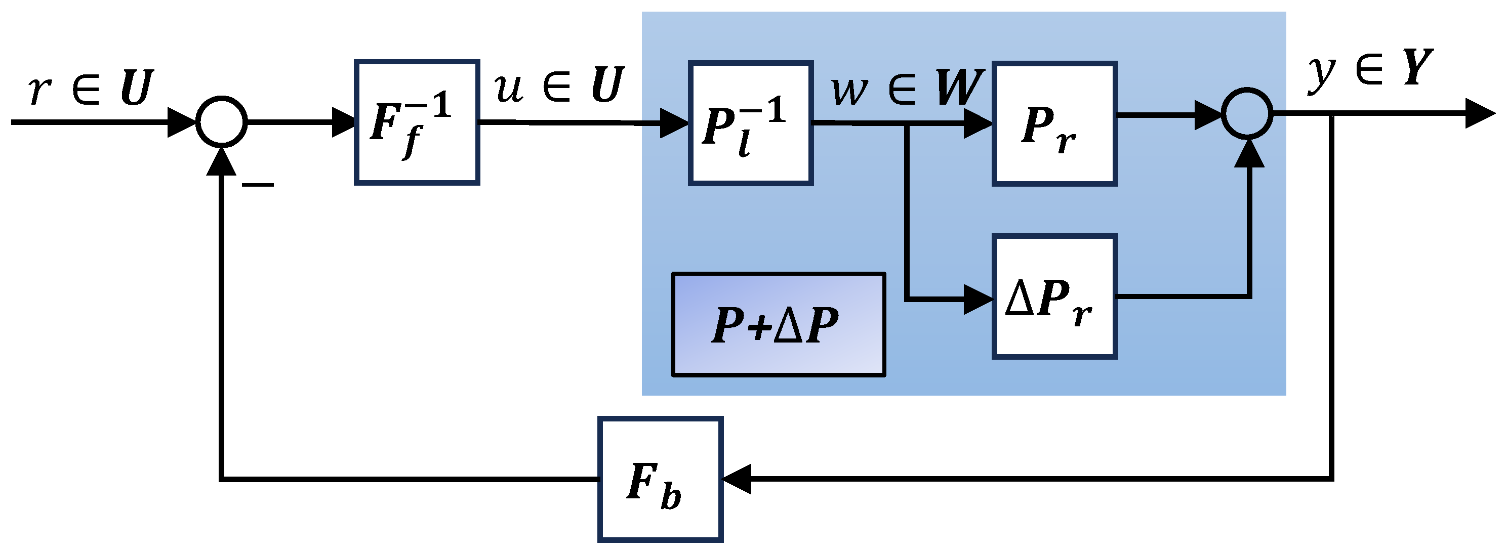
Based on Lemma 1, the feedback system shown in Figure 1 can be equivalently transformed to the system shown in Figure 2. The relationship between plant output and the reference input can be stated as

Figure 2.
Equivalent right coprime factorization of nominal plant.
Definition 7.
Let and be two extended linear spaces, which are associated, respectively, with two given Banach spaces and of measurable functions defined on the time domain . Let be a subset of ; a nonlinear operator is called a generalized Lipschitz operator on if there exists a constant L such that
for all . denotes the family of nonlinear generalized Lipschitz operators that map to itself. Note that the least such constant L is given by
It should be noted that the internal signals in real systems are required to be uniquely determined, whereas non-unique outputs from an input may be produced by a nonlinear operator, especially for a set-valued mapping. But the introduction of generalized Lipschitz operator can guarantee the uniqueness requirement.
Lemma 2.
Let and be Banach spaces, is an invertible operator, and R is an operator in , such that where . Then, the operator is invertible in and
3. Main Results
In this section, prior to introducing the control design for the plant with sundry disturbed open loop dynamics, we will recall the approach of robust right coprime factorization for the perturbed plant that has been described in [25], where the disturbed open loop dynamics position in the feed forward path.
Firstly, the definition of disturbed open loop dynamics used in this paper is depicted.
Definition 8.
is the disturbed open loop dynamics, which are commonly presumed to fall within a specific compact and convex set Δ, namely
and this set Δ is called the set of disturbed open loop dynamics. ‘open loop’ means the disturbed dynamics occur in separate units of the system.
The disturbed open loop dynamics are used in this section.
The conventionally employed robust right coprime factorization approach can be summarized as follows.
Lemma 3.
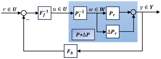
For the disturbed open loop dynamics, due to uncertainties or disturbances, assuming that the disturbed open loop dynamics is bounded, then the plant with disturbed open loop dynamics can be represented as , where is a stable and bounded operator. By employing the robust right coprime factorization approach, as shown in Figure 3, let the Bezout identity of nominal plant be and the plant with disturbed open loop dynamics be , respectively. If the following inequality is satisfied,
then the system shown in Figure 3 is stable. In other words, the plant with disturbed open loop dynamics is said to remain robust right coprime factorization. are unimodular operators, is the Lipschitz norm.

Figure 3.
Robust right coprime factorization of the plant with disturbed open loop dynamics that locate in the feed forward path.
In such a robust right coprime factorization approach, the disturbed open loop dynamics due to uncertainties or disturbances are only located in feed forward path and summarized into . A condition in the form of inequality guarantees the robust stability of the plant with disturbed open loop dynamics. However, this is not a universal scenario in practical systems, since the disturbed open loop dynamics may also appear in the feedback path during the process of signal transformation. In this work, disturbed open loop dynamics located in both the feed forward path and feedback loop are considered. The disturbed open loop dynamics are commonly as a result of sensor noise, time delay and other disturbances. For the disturbed open loop dynamics in feedback loop, if there exists an operator that can enable the signal in the feedback path an identity, namely, the mapping from plant output to the controller is an identity, then the reconfiguration of controllers in preceding path and response loop designed at the outset using robust right coprime factorization can be avoided. Generally, there are some appropriate approaches such as disturbance observer and filter method that can be employed to achieve an identity in the feedback loop signal transformation. An ideal such perturbation eliminator empowers the signal in the feedback circuit an identity even in the presence of disturbed dynamics. This allows designers to layout controllers without considering the interference of disturbed open loop dynamics.
The control system can be designed as Figure 4, where the sundry disturbed open loop dynamics are located in and F. The operator F is composed of disturbed open loop dynamics and the elimination of the adverse effect of disturbed dynamics, which enables the projection an identity in the presence of disturbed open loop dynamics. If such an objective can be achieved ideally, conceptually, it can say that . Thus, the controllers designed using robust right coprime factorization can remain the original ones.
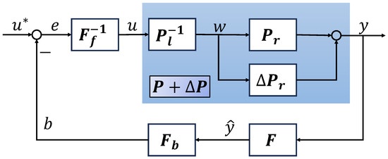
Figure 4.
Ideal control design scheme for system with sundry disturbed open loop dynamics.
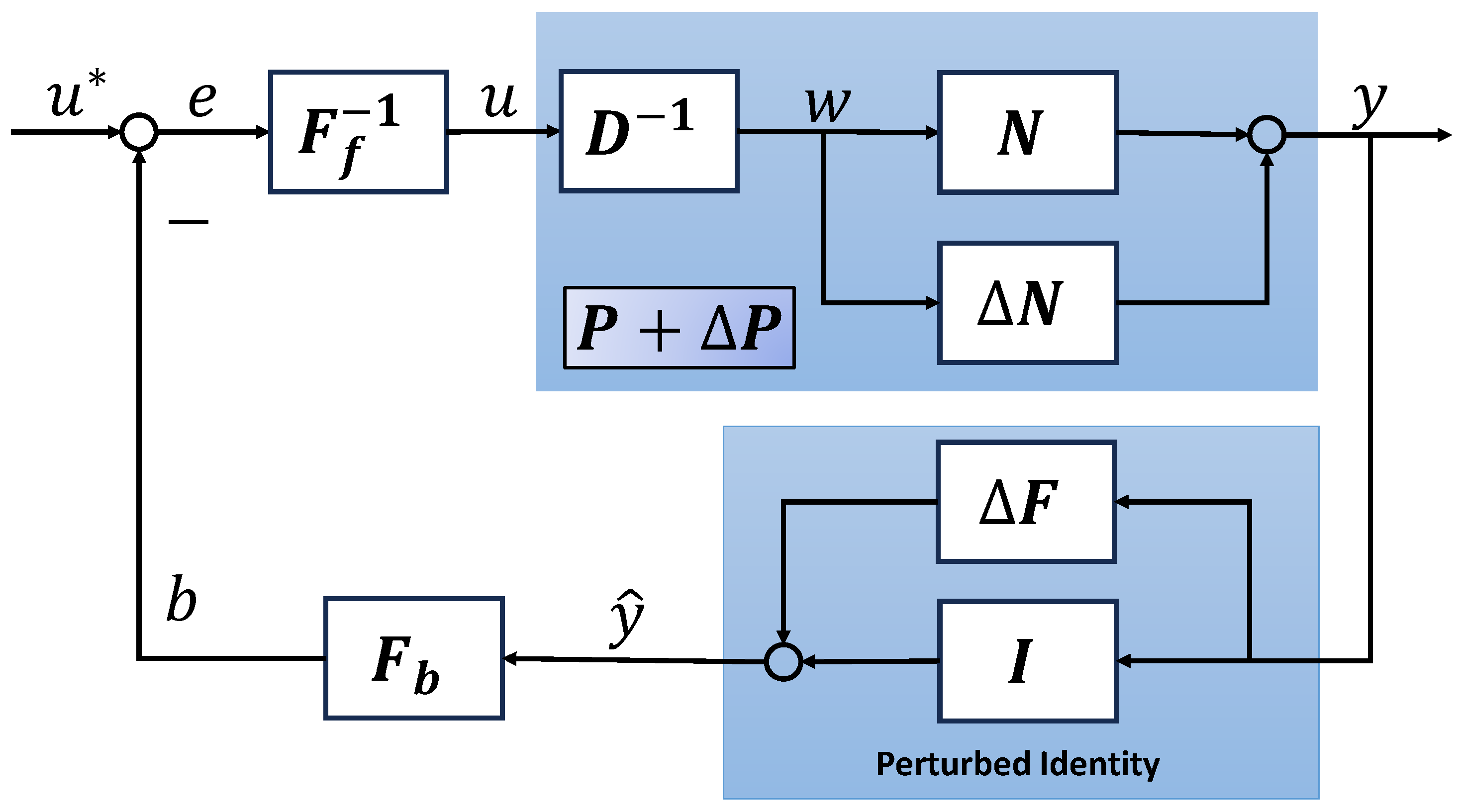
It should be noted that such ideal operators F are almost non-existent, seeing that the results estimated by disturbance observer or filter method typically take some time to converge to the true value or converge within a certain neighborhood, thus the identity mapping can hardly be ensured. For such disturbed open loop dynamics, a new control system design scheme is shown in Figure 5, which is a design scheme of more practical significance. From the figure, a perturbed identity denoted as is employed where is stable and bounded. The robust stability of the system can be guaranteed by using robust right coprime factorization based on a new perturbed Bezout identity and a condition in the form of inequality as follows.
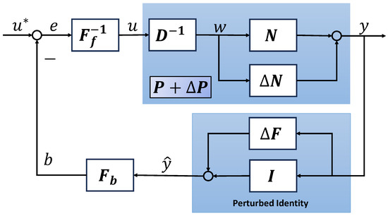
Figure 5.
Control design scheme for system with sundry disturbed open loop dynamics.
Theorem 1.
Let be a linear subspace of the extended linear space associated with a given Banach space , and let . Let the Bezout identity of the nominal plant be , and the exact system with sundry disturbed open loop dynamics be , respectively. Then, the system shown in Figure 5 is stable or the system is said to remain robust right coprime factorization if
where is an unimodular operator, is Lipschitz norm.
Proof.
M is an unimodular operator, which implies its invertibility. Since
Then, we have
and
then, is invertible based on Lemma 2, where I is the identity operator. Thus, we have
Meanwhile, since and , then , provided that the system in Figure 5 is well-posed. As a result, for any . Further, since and , the stability of and implies that and . Then, the system is overall stable. ☐
Compared with the robust stability condition of the plant with disturbed open loop dynamics that only locate in the feed forward, the above condition is in a new inequality form, which shows that it includes more sets for designing controllers. That is, (9) includes the robust stability condition . Additionally, if the condition can be satisfied by using the bounded information of , then the detailed information of is not essential. In comparison with the robust stability condition proposed in [31], where the disturbed open loop dynamics are all related with the plant, the robust right coprime factorization approach in a new form proposed in this paper also expands the range of control for plant with sundry disturbed open loop dynamics, since the backward disturbed open loop dynamics can be plant-independent.
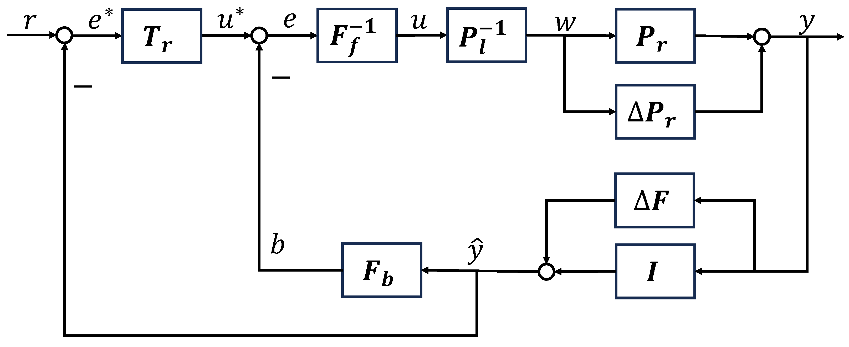
After the robust stability of the plant with sundry disturbed open loop dynamics has been guaranteed by satisfying a condition formulated in a new inequality form, as described in Figure 5 and Theorem 1, the tracking performance of the overall system is considered. For the tracking performance, the system design scheme is shown in Figure 6, where is a tracking operator to ensure the output of the plant y can track the reference input r. The tracking controller is designed as
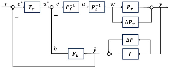
Figure 6.
Tracking design scheme for system with sundry disturbed open loop dynamics.
4. Numerical Examples
Within this part, we present two numerical examples: one for the water level compensation system and the other for the heat exchange process. These examples serve to demonstrate the effectiveness of the proposed robust stability condition in RRCF approach. For detailed system descriptions, please refer to Appendix A and Appendix B.
4.1. Case 1: Water Level Compensation System
Utilizing right coprime factorization, for controlling the nominal water level compensation system is designed as
The factorization of the plant with disturbed open loop dynamics is represented as follows:
where represents the open loop dynamics in the forward path. The disturbed open loop dynamics in the feedback loop is much more complex, and it is because of unknown time-varying delay and strong sensor noise. Then, controllers are designed as followings where K is a design parameter.
For achieving the tracking performance, is designed using the method outlined in Section 3.
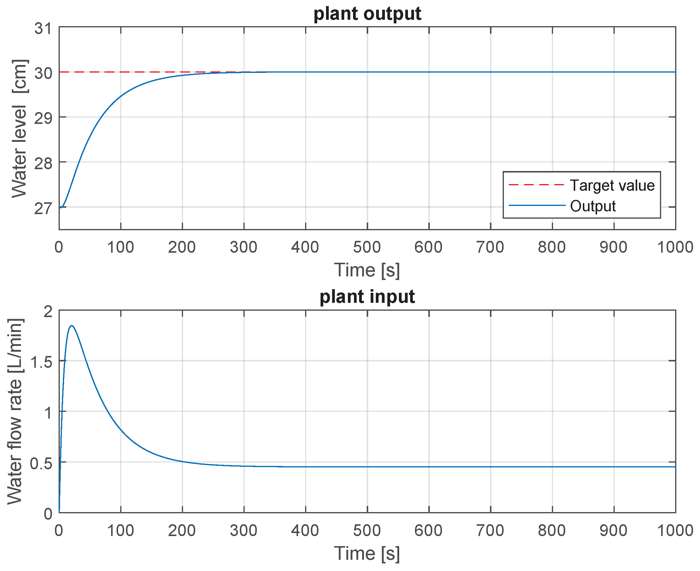
The initial water level of Tank1 is set to be 27 cm. The flow rate is regulated within the range of [0, 2.0 L/min] by the attached valve, with the target water level being r = 30 cm. The disturbed open loop dynamics in the feed forward is set as . In the feedback path, the disturbed open loop dynamics in the form of time-varying delay is subjected to Gaussian distribution with a maximum of 15 s. The disturbed open loop dynamics in the form of the strong sensor noise is white noise, with mean and variance . For dealing with such complex disturbed open loop dynamics, a variant of particle filter algorithm (described in Appendix C) is used to achieve a disturbed identity operator , as illustrated above, where the effect of time delay and sensor noise are dealt with at the same time. In particle filter, the process noise is assumed with mean and variance , respectively. The other simulation parameters are listed in Table A1.
The simulation results of the plant output and input are presented in Figure 7. As depicted, the water level compensation system demonstrates stability and ultimately achieves tracking of the target value within finite time.
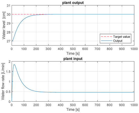
Figure 7.
Simulation results of plant with sundry open loop dynamics.
The robust stability of the control system was verified using the proposed robust stability condition outlined in Theorem 1 (or (9)). The results are illustrated in Figure 8. Throughout the entire simulation duration, the Lipschitz norm remains below 1. Consequently, the figure confirms the guaranteed robust stability.
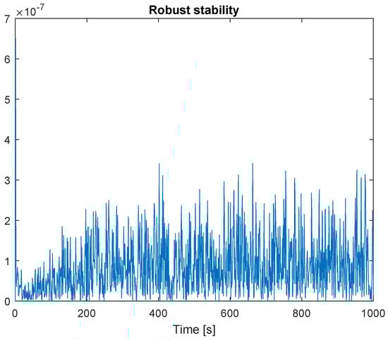
Figure 8.
Robust stability.
4.2. Case 2: Heat Exchange Process with a Spiral Heat Exchanger
The heat exchange process with a spiral heat exchanger system, which includes uncertainty [33], and undergoes robust right factorization and stabilization, denoted as (18).
where K is the design parameter, and
For achieving the tracking performance, is designed using the method outlined in Section 3.
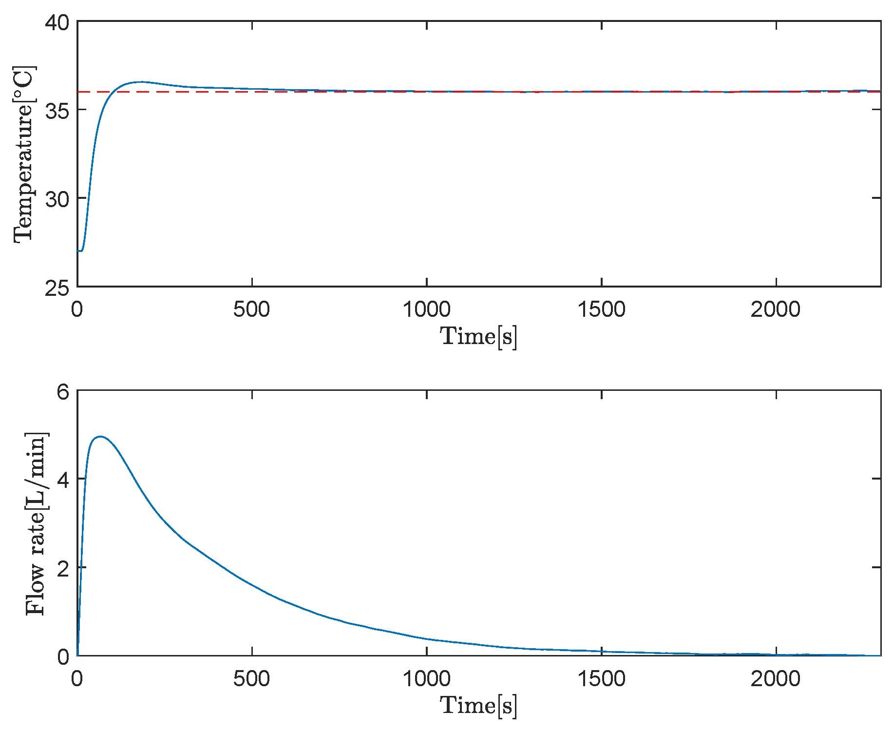
The parameters are provided in Table A2. The hot fluid flow rate maximum value is 5.6 L/min, and the cold fluid flow rate maximum value is 4.5 L/min, respectively. The input and output variables are and . The plant input is subject to disturbed open-loop dynamics in the feed forward path attributed to white noise with mean and variance . The plant output value is affected by disturbed open-loop dynamics in the feedback loop caused by white sensor noise with mean and variance , along with Gaussian distributed time-varying delay with a maximum delay of 15 s. For addressing the impact of disturbed open loop dynamics in the form of strong sensor noise and time-varying delay at the same time in the feedback loop, the particle filter variant algorithm (described in Appendix C) is employed to acquire a disturbed identity operator . In the particle filter variant, the process noise is assumed with mean and variance , respectively.
The simulation results of the plant output and plant input are depicted in Figure 9. It is evident that the heat exchange process remains stable, and the tracking performance is assured.
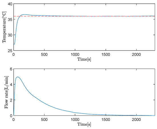
Figure 9.
Simulation results of heat exchange process with sundry disturbed open loop dynamics.
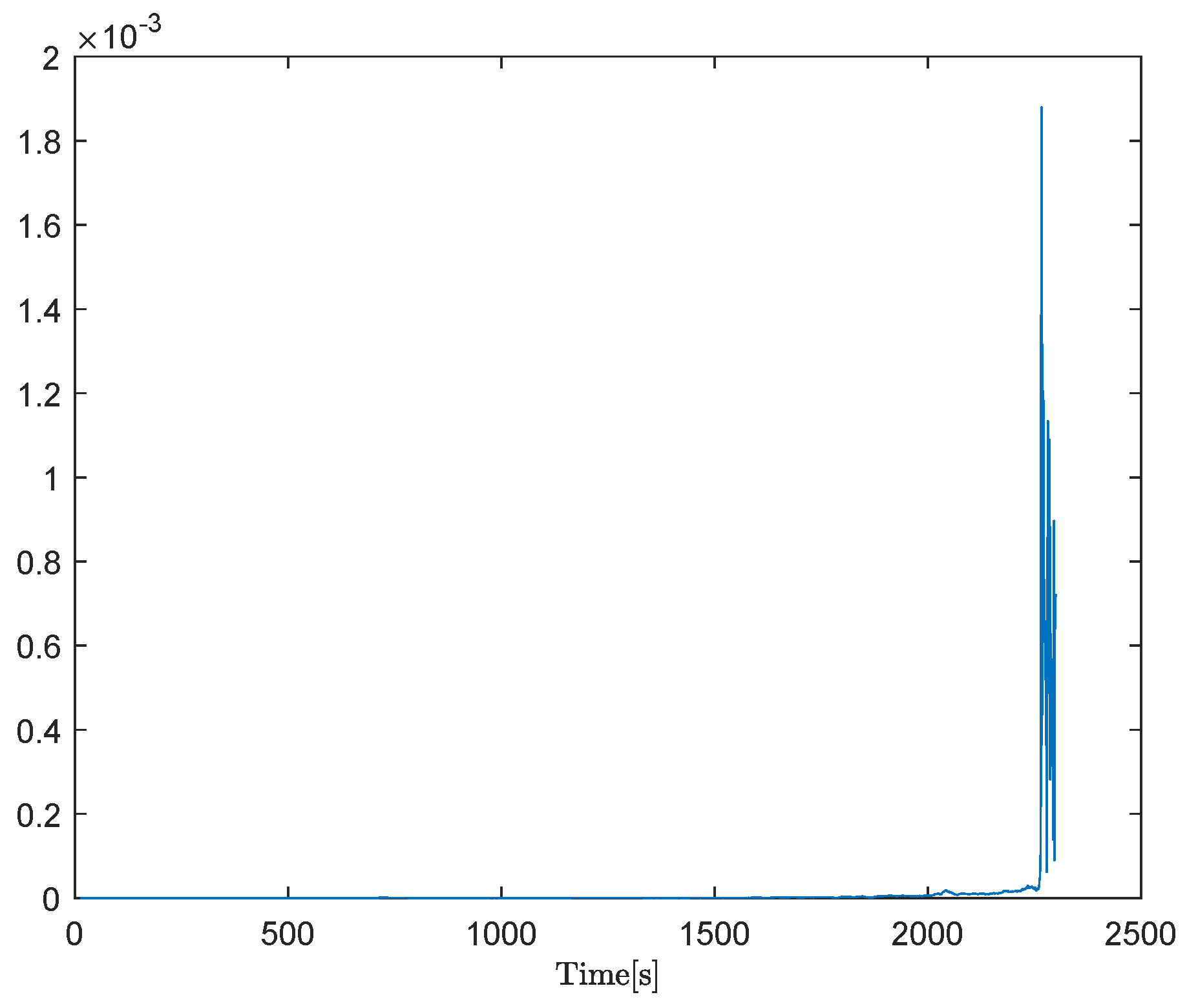
Taking into account the sundry disturbed open-loop dynamics located in the feed forward and feedback loops, stability is ensured by Theorem 1 (or (9)). Figure 10 corroborates the efficacy of the proposed approach, wherein the Lipschitz norm consistently remains below 1, aligning with the conditions stipulated in Theorem 1.
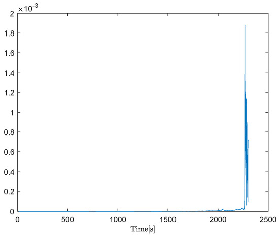
Figure 10.
Robust stability of heat exchange process with sundry disturbed open-loop dynamics.
5. Conclusions and Discussions
In this paper, robustness for a plant with sundry disturbed open loop dynamics is analyzed by using robust right coprime factorization approach. Different from the previous methodologies where the disturbed open loop dynamics typically reside in the feedforward path, and a disturbed Bezout identity, along with an inequality condition, is employed to ensure robust stability, this work introduces a new condition. That is, a robust stability condition in the form of a new disturbed Bezout identity coupled with a new stability inequality is proposed to ensure the robust stability of the plant with sundry disturbed open loop dynamics both in feed forward and feedback loops. Two numerical examples illustrate the effectiveness of the proposed approach.
The proposed robust stability condition in the approach of robust right coprime factorization broadens the scope of controller designs to encompass the disturbed open loop dynamics, whether they are related or unrelated to the plant. Additionally, the proposed robust stability condition can be readily implemented for real-time control applications. In various industrial domains, linearization is a commonly employed technique where system approximation is necessary, and closed-loop stability analysis is essential for controllers designed based on the linearized plant. In case of smooth nonlinearities, it is feasible to use a linearized plant with structured uncertainty and to design simply an or controller. Hence, there is merit in exploring nonlinear control approaches based on linearization and the proposed condition outlined in this paper in future research endeavors.
Author Contributions
Methodology, Y.X. and M.D.; software, Y.X.; validation, Y.X.; formal analysis, Y.X.; investigation, Y.X.; resources, M.D.; writing—original draft preparation, Y.X.; writing—review and editing, Y.X. and M.D.; supervision, M.D. All authors have read and agreed to the published version of the manuscript.
Funding
This research received no external funding.
Data Availability Statement
Data sharing is not applicable to this article due to privacy considerations.
Conflicts of Interest
The authors declare no conflicts of interest.
Appendix A. Water Level Compensation System
The water level compensation system is depicted in Figure A1 [34]. This system comprises two interconnected tanks: Tank1 (the outer large tank) and Tank2 (the inner small tank), where Tank2 is situated within Tank1. There is a hole in the bottom surface of Tank1, through which liquid can be discharged, and the outflow rate from Tank1 can be regulated using a valve. The discharged liquid is collected in a container located at the bottom of Tank1. Similarly, a hole in the top of Tank1 allows liquid to be pumped from the container using a pump. To maintain a constant liquid level in Tank1, liquid is continuously injected to compensate for any changes in level, and the pump ensures a constant flow rate by pumping a fixed amount of liquid. Control over the amount of liquid entering Tank1 is achieved through the valve connected to the pump. The water enters Tank1 at a constant flow rate from its bottom and subsequently flows out from its top.
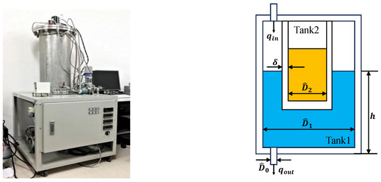
Figure A1.
Water level compensation system.
Figure A1.
Water level compensation system.
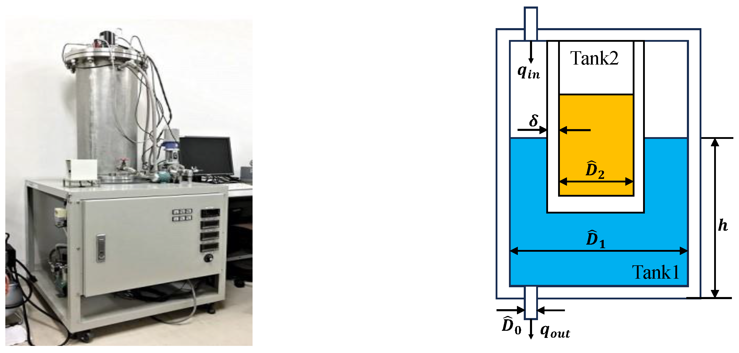
The water level compensation system is modeled as
where the input is the water input flow of Tank1, and is the water level h of Tank1. The parameters used in the model of the water level compensation system are defined in Table A1.

Table A1.
Simulation parameters of water level compensation system.
Table A1.
Simulation parameters of water level compensation system.
| T | simulation time | 1000 | [s] |
| sampling period | 1 | ||
| proportional gain | |||
| integral gain | |||
| K | designed parameter | ||
| thickness of sold wall | 2 | [cm] | |
| h | water level in Tank1 | [cm] | |
| v | outflow rate | [cm/s] | |
| water inflow of Tank1 | [L/min] | ||
| water outflow of Tank1 | [L/min] | ||
| Tank1 outlet inner diameter | [cm] | ||
| Tank1 inner diameter | [cm] | ||
| Tank2 inner diameter | [cm] | ||
| g | gravity acceleration | [cm/s2] |
Appendix B. Heat Exchange Process with a Spiral Heat Exchanger
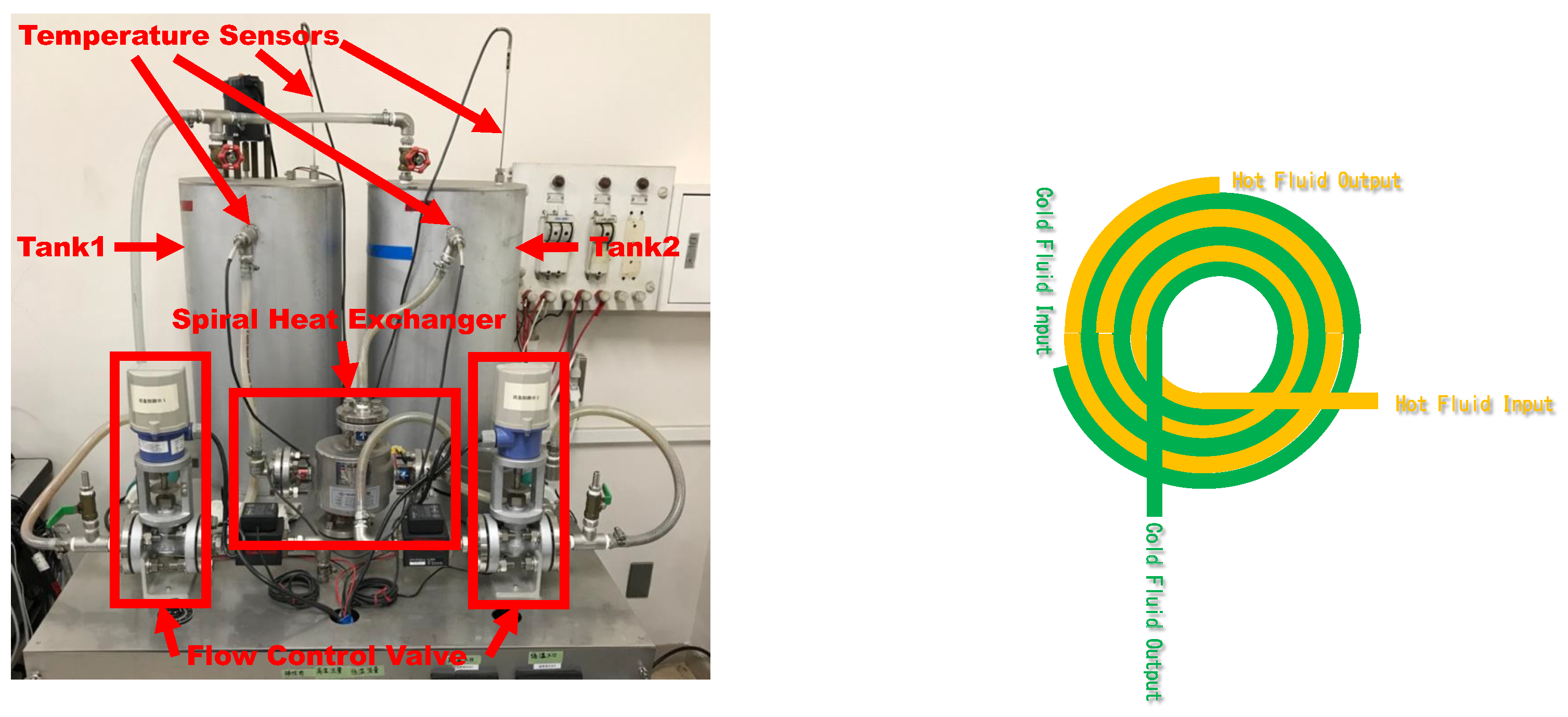
Figure A2 depicts the plant of a heat exchange process featuring a spiral heat exchanger. In this configuration, the heat exchange process does not necessitate the mixing of the hot fluid in Tank1 and the cold fluid in Tank2; instead, each type of fluid returns to its respective tank. A flow control valve regulates the flow rate of each fluid, with its operation commanded by an analog current signal. Temperature sensors are positioned at four locations to measure the following temperatures within the spiral heat exchanger: cold fluid inlet temperature , cold fluid outlet temperature , hot fluid inlet temperature , and hot fluid outlet temperature of the spiral heat exchanger. It is worth noting that is considered constant.
The heat exchanger can be modeled according to the following equation. The parameters for this model are provided in Table A2.

Table A2.
Simulation parameters for the heat exchange process.
Table A2.
Simulation parameters for the heat exchange process.
| r | Target temperature value | 36 °C |
| Hot fluid outlet temperature | 41 °C | |
| Initial cold fluid inlet temperature | 27 °C | |
| Initial cold fluid temperature | 27 °C | |
| a | Archimedes’ spiral equation constant | m/rad |
| Thermal conductivity of SUS304 | 16.7 W/(m · °C) | |
| Reynolds number | 22,000 | |
| Prandtl number | 7 | |
| B | Cross-section area of flow path | m2 |
| Specific heat of water | 4.2 kJ/(kg · °C) | |
| Density of water | 1000 kg/m3 | |
| Thickness of heat exchanger’s wall | m | |
| Width of flow path | m | |
| m | Mass of cold fluid flow rate | 0.0717 kg |
| M | Mass of cold fluid in Tank2 | 31.8 kg |
| - Design parameter | 0.3 L/min | |
| - Design parameter | 0.03 | |
| Design parameter for valve of hot fluid | 1.25 | |
| Design parameter for flow change of hot fluid | 0.026 | |
| K | Design parameter of | 0.7 |
| Proportional gain of C | 2000 | |
| Integral gain of C | 97 | |
| Sampling time | 1 s | |
| Simulation time | 2301 s | |
| Standard deviation of likelihood function | 0.01 °C |
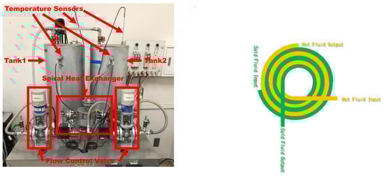
Figure A2.
Heat exchange process with a spiral heat exchanger.
Figure A2.
Heat exchange process with a spiral heat exchanger.
Appendix C. Variant of Particle Filter Algorithm
A dynamic statistical system expressed as state space is described as
where , , , , denote the process model, measurement model, control input, the state, and output correspondingly. The process model noise and measurement noise are assumed to be independent and identically distributed, complying with any given distribution. The posterior probability distribution of the initial state is considered to follow a Gaussian distribution [35].
A particle filter estimates posterior distribution via weighted samples drawn from an importance proposal distribution . The weight of every sample can be recursively calculated as
Here, represents likelihood and represents prior distribution. The importance proposal distribution is selected as . Then, (A4) can be written as
The state is estimated by the summation of weighted samples
where
In the variant of the particle filter algorithm, the residual is calculated using the absolute difference between the measured value and sampled particles. The strength of is evaluated using the rule. If the number of particles violating the rule exceeds some threshold, exponential weights are designated to particles beyond the boundary. For particles within the range, their weights remain unchanged. Particle weights are calculated using (A8). Then, the exponential weights and original ones are normalized for the subsequent estimation as (A6) and (A7) [33].
References
- Åström, K.J. Introduction to Stochastic Control Theory; Courier Corporation: North Chelmsford, MA, USA, 2012. [Google Scholar]
- Zheng, K.; Shi, D.; Hirche, S.; Shi, Y. Innovation-triggered Learning for Data-driven Predictive Control: Deterministic and Stochastic Formulations. arXiv 2024, arXiv:2401.15824. [Google Scholar]
- Zhou, K.; Doyle, J.C. Essentials of Robust Control; Prentice Hall: Upper Saddle River, NJ, USA, 1998; Volume 104. [Google Scholar]
- Yan, Y.; Wang, X.F.; Marshall, B.J.; Liu, C.; Yang, J.; Chen, W.H. Surviving disturbances: A predictive control framework with guaranteed safety. Automatica 2023, 158, 111238. [Google Scholar] [CrossRef]
- Nikiforov, V.O. Nonlinear servocompensation of unknown external disturbances. Automatica 2001, 37, 1647–1653. [Google Scholar] [CrossRef]
- Bodson, M.; Jensen, J.S.; Douglas, S.C. Active noise control for periodic disturbances. IEEE Trans. Control Syst. Technol. 2001, 9, 200–205. [Google Scholar] [CrossRef]
- Back, J.; Shim, H. Adding robustness to nominal output-feedback controllers for uncertain nonlinear systems: A nonlinear version of disturbance observer. Automatica 2008, 44, 2528–2537. [Google Scholar] [CrossRef]
- Arias, G. Stabilization of a microbeam model with distributed disturbance. Syst. Control Lett. 2023, 173, 105466. [Google Scholar] [CrossRef]
- Modares, H. Data-driven Safe Control of Uncertain Linear Systems Under Aleatory Uncertainty. IEEE Trans. Autom. Control 2023, 69, 551–558. [Google Scholar] [CrossRef]
- Ahmadi, M.; Rosolia, U.; Ingham, M.D.; Murray, R.M.; Ames, A.D. Risk-Averse Decision Making Under Uncertainty. IEEE Trans. Autom. Control 2023, 69, 55–68. [Google Scholar] [CrossRef]
- Ebeigbe, D.; Nguyen, T. On Robust Control with Uncertainties in the Regressor Matrix and Parameter Vector. IEEE Trans. Autom. Control 2023, 69, 309–314. [Google Scholar] [CrossRef]
- Kwak, D.; Kim, J.H.; Hagiwara, T. Robust Stability Analysis of Sampled-Data Systems with Uncertainties Characterized by the L-infinity-induced Norm: Gridding Treatment with Convergence Rate Analysis. IEEE Trans. Autom. Control 2023, 68, 8119–8125. [Google Scholar] [CrossRef]
- Sibai, H.; Mitra, S. State Estimation of Continuous-time Dynamical Systems with Uncertain Inputs with Bounded Variation: Entropy, Bit Rates, and Relation with Switched Systems. IEEE Trans. Autom. Control 2023, 68, 7041–7056. [Google Scholar] [CrossRef]
- Ning, B.; Han, Q.L.; Sanjayan, J.; Shang, W.; Lam, W.Y. Robust trajectory tracking control for cable-driven parallel robots with model uncertainty. Control Eng. Pract. 2023, 140, 105662. [Google Scholar] [CrossRef]
- Liu, H.; Li, Y.; Han, Q.L.; Ra, T. Watermark-based Proactive Defense Strategy Design For Cyber-Physical Systems With Unknown-but-bounded Noises. IEEE Trans. Autom. Control 2022, 68, 3300–3315. [Google Scholar] [CrossRef]
- Rizvi, S.A.A.; Pertzborn, A.J.; Lin, Z. Reinforcement learning based optimal tracking control under unmeasurable disturbances with application to HVAC systems. IEEE Trans. Neural Netw. Learn. Syst. 2021, 33, 7523–7533. [Google Scholar] [CrossRef] [PubMed]
- Meng, T.; Xie, Y.; Lin, Z. Consensus of Linear Multi-Agent Systems in the Presence of Bounded Measurement Noises. In Proceedings of the 2020 39th Chinese Control Conference (CCC), Shenyang, China, 27–29 July 2020; pp. 5128–5133. [Google Scholar]
- Rsetam, K.; Cao, Z.; Man, Z. Design of robust terminal sliding mode control for underactuated flexible joint robot. IEEE Trans. Syst. Man Cybern. Syst. 2021, 52, 4272–4285. [Google Scholar] [CrossRef]
- Wang, H.; Man, Z.; Kong, H.; Zhao, Y.; Yu, M.; Cao, Z.; Zheng, J.; Do, M.T. Design and implementation of adaptive terminal sliding-mode control on a steer-by-wire equipped road vehicle. IEEE Trans. Ind. Electron. 2016, 63, 5774–5785. [Google Scholar] [CrossRef]
- Chen, J.; Qian, D. Three controllers via 2nd-order sliding mode for leader-following formation control of multi-robot systems. Int. J. Adv. Mechatron. Syst. 2021, 9, 85–101. [Google Scholar] [CrossRef]
- Guzmán, P.; Prieur, C. Rapid stabilization of a reaction-diffusion equation with distributed disturbance. In Proceedings of the 2020 59th IEEE Conference on Decision and Control (CDC), Jeju, Republic of Korea, 14–18 December 2020; pp. 666–671. [Google Scholar]
- Pisano, A.; Orlov, Y. Boundary second-order sliding-mode control of an uncertain heat process with unbounded matched perturbation. Automatica 2012, 48, 1768–1775. [Google Scholar] [CrossRef]
- Ferrara, A.; Incremona, G.P.; Vecchio, C. Adaptive Multiple-Surface Sliding Mode Control of Nonholonomic Systems with Matched and Unmatched Uncertainties. IEEE Trans. Autom. Control 2023, 69, 614–621. [Google Scholar] [CrossRef]
- Deng, M.; Inoue, A.; Goto, S. Operator based thermal control of an aluminum plate with a Peltier device. Int. J. Innov. Comput. Inf. Control 2008, 4, 3219–3229. [Google Scholar]
- Deng, M.; Inoue, A.; Ishikawa, K. Operator-based nonlinear feedback control design using robust right coprime factorization. IEEE Trans. Autom. Control 2006, 51, 645–648. [Google Scholar] [CrossRef]
- An, Z.; Bu, N. Modeling for a Bellow-Shaped Soft Actuator Based on Yeoh model and Operator-Based Nonlinear Control Design. In Proceedings of the 2023 International Conference on Advanced Mechatronic Systems (ICAMechS), Melbourne, Australia, 4–7 September 2023; pp. 1–5. [Google Scholar]
- Bu, N.; Liu, H.; Li, W. Robust passive tracking control for an uncertain soft actuator using robust right coprime factorization. Int. J. Robust Nonlinear Control 2021, 31, 6810–6825. [Google Scholar] [CrossRef]
- Deng, M.; Iwai, Z.; Mizumoto, I. Robust parallel compensator design for output feedback stabilization of plants with structured uncertainty. Syst. Control Lett. 1999, 36, 193–198. [Google Scholar] [CrossRef]
- Deng, M.; Inoue, A.; Zhu, Q. An integrated study procedure on real-time estimation of time-varying multi-joint human arm viscoelasticity. Trans. Inst. Meas. Control 2011, 33, 919–941. [Google Scholar] [CrossRef]
- Bu, N.; Wang, X. Swing-up design of double inverted pendulum by using passive control method based on operator theory. Int. J. Adv. Mechatron. Syst. 2023, 10, 1–7. [Google Scholar] [CrossRef]
- Li, M.; Deng, M. Operator-based external disturbance rejection of perturbed nonlinear systems by using robust right coprime factorization. Trans. Inst. Meas. Control 2018, 40, 3169–3178. [Google Scholar] [CrossRef]
- Gao, X.; Yang, Q.; Zhang, J. Multi-objective optimisation for operator-based robust nonlinear control design for wireless power transfer systems. Int. J. Adv. Mechatron. Syst. 2022, 9, 203–210. [Google Scholar] [CrossRef]
- Xu, Y.; Deng, M. Particle filter design for robust nonlinear control system of uncertain heat exchange process with sensor noise and communication time delay. Appl. Sci. 2022, 12, 2495. [Google Scholar] [CrossRef]
- Kochi, R.; Deng, M. Multivariable Fractional-Order Controller Design of Nonlinear Dual Tank Device. Fractal Fract. 2024, 8, 27. [Google Scholar] [CrossRef]
- Arulampalam, M.S.; Maskell, S.; Gordon, N.; Clapp, T. A tutorial on particle filters for online nonlinear/non-Gaussian Bayesian tracking. IEEE Trans. Signal Process. 2002, 50, 174–188. [Google Scholar] [CrossRef]
Disclaimer/Publisher’s Note: The statements, opinions and data contained in all publications are solely those of the individual author(s) and contributor(s) and not of MDPI and/or the editor(s). MDPI and/or the editor(s) disclaim responsibility for any injury to people or property resulting from any ideas, methods, instructions or products referred to in the content. |
© 2024 by the authors. Licensee MDPI, Basel, Switzerland. This article is an open access article distributed under the terms and conditions of the Creative Commons Attribution (CC BY) license (https://creativecommons.org/licenses/by/4.0/).


