Fog, Friction, and Failure in Organized Conflict: A Formal Study

Abstract

Organized conflict, while confined by the laws of physics—and, under profound strategic incompetence, by the Lanchester equations—is not a physical process but rather an extended exchange between cognitive entities that have been shaped by path-dependent historical trajectories and cultural traditions. Cognition itself is confined by the necessity of duality, with an underlying information source constrained by the asymptotic limit theorems of information and control theories. We introduce the concept of a ‘basic underlying probability distribution’ characteristic of the particular cognitive process studied. The dynamic behavior of such systems is profoundly different for ‘thin-tailed’ and ‘fat-tailed’ distributions. The perspective permits the construction of new probability models that may provide useful statistical tools for the analysis of observational and experimental data associated with organized conflict, and, in some measure, for its management.

1. Introduction

…To succeed in strategy you do not have to be distinguished or even particularly competent. All that is required is performing well enough to beat an enemy. You do not have to win elegantly; you just have to win.

—C. S. Gray [1].

Organized conflict is a quintessential example of embodied cognition at and across various scales and levels of organization, from individual combatants, their squads, and their platoons, through a hierarchy of larger elements, including armies embedded within a central and overarching polity engaged in a discourse of ‘politik’ with one or more others.

Each element, at each scale, can be viewed as a cognitive entity embedded in a ‘Clausewitz landscape’ of fog, friction, and skilled adversarial intent that has been the study of practitioners across a rich variety of times, places, and cultural milieus [2,3,4].

The most usual formal treatment of these matters has involved the dynamic attrition models pioneered by Osipov [5] and Lanchester [6], as extended and applied by many others [7,8,9,10,11,12].

It is worth outlining the basic Lanchester model [13] because it applies most particularly to grinding World War I trench warfare circumstances of attritional stalemate that are widely viewed as a strategic catastrophe, most often a consequence of strategic incompetence.

The basic model assumes that, at time $t=0$, there are $A_0$ and $B_0$ combatants. Dynamics occur according to the relations

$$dA\left(t\right)/dt=-\beta B\left(t\right)$$

$$dB\left(t\right)/dt=-\alpha A\left(t\right)$$

This ‘simple’ model leads to the following conclusions, the first three of which are obvious:

I.

If $\alpha =\beta$, then the side with more combatants at $t=0$ wins.

II.

If $A_0=B_0$, the side with greater firepower wins.

III.

If $A_0>B_0$ and $\alpha >\beta$, then A wins. If, however, $A_0<B_0$ and $\alpha <\beta$, then B wins.

IV.

If $A_0>B_0$ but $\alpha <\beta$, or if $A_0<B_0$ but $\alpha >\beta$, the winning side depends of whether the ratio $\beta /\alpha$ is greater or less than ${(A_0/B_0)}^2$. This is Lanchester’s ‘Square Law’.

Current research, cited above, replicates these results in more terms and sometimes to a higher order. The work by Osipov and Lanchester more than a century ago, sadly, remains both foundational and relevant.

Here, in some contrast to such work—in the absence of, or simply tangential or orthogonal to, this mode of strategic incompetence and catastrophe—we explore the dynamics of embodied cognition on landscapes of ‘fog’, ‘friction’, and deadly adversarial intent, in which both incoming ‘sensory information’ and ‘materiel’ resources needed for successful address of patterns of threat and affordance are delayed and blurred by ‘noise’. This is achieved by taking perspectives based on the asymptotic limit theorems of information and control theories, as extended by methods familiar from statistical physics that will be described in more detail below.

In particular, our approach is consonant with the work of Atlan and Cohen [14], who invoked a ‘cognitive paradigm’ for the immune system. This complex physiological entity receives something much like sensory information regarding both routine cellular maintenance and pathogenic attack; compares that information with an inherited or learned picture of the world (innate or acquired immunity); and, using that comparison, chooses a small set of actions from a much larger repertoire of those available to it among the various forms and targets of inflammation. Such choice reduces uncertainty, and the reduction in uncertainty implies the existence of an information source ‘dual’ to the cognitive process of choice. Much the same was described by Dretske [15] some years ago.

This process can, we will show, be interpreted via the Rate Distortion Theorem (RDT) of information theory [16] that determines the minimum channel capacity needed to limit some particular measure of average distortion between what has been ordered and what has been observed to a given scalar limit.

Following the tradition of Feynman [17] and Bennett [18], we view information channel capacity as another form of free energy and iterate the argument to a higher order via standard methods from statistical physics [19] that permit the imposition of dynamics under an analog to the Onsager approximation to nonequilibrium thermodynamics [20]. The approach is based, however, on a system’s underlying probability distribution that may be very different from the Boltzmann (or Exponential) of ‘ordinary’ physics. Indeed, such ‘cognitive’ distributions may be burdened (or enhanced, depending on your perspective), by ‘fat tails’ in the sense of Taleb [21] and Derman et al. [22]—representing high kurtosis and jump diffusion—that impose a qualitatively different form of ‘noise’ onto the fog-and-friction of real-world, real-time conflict.

2. The Rate Distortion Theorem

The RDT states that, for a given acceptable scalar measure of distortion D between a sequence of signals that has been ‘sent’ and the sequence that has actually been ‘received’ in message transmission—the gap between what was wanted and what was obtained—there is a minimum necessary channel capacity $R\left(D\right)$ in the classic information theory sense that is determined by the rate at which essential resources, indexed by some particular scalar measure Z, are provided to the system ‘sending the message’ in the presence of ‘noise’.

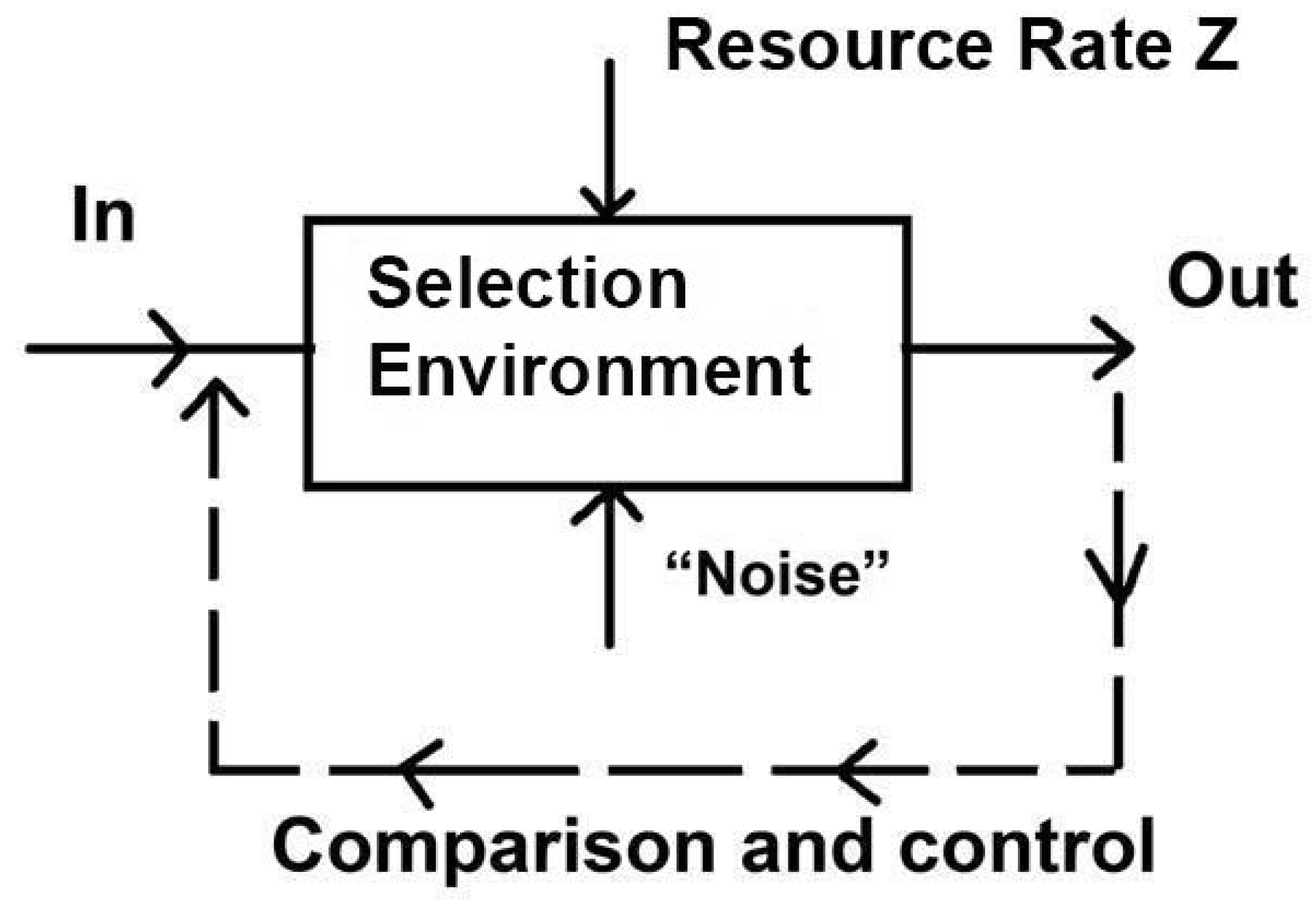
Figure 1 displays the basic model as we will apply it here. A sequence of intent signals from a cognitive entity is transmitted on the timescale of interest into a ‘selection environment’ represented by the rectangle. A scalarized measure of resource delivery rate, Z, is opposed by a ‘noise’ compounded of uncertainties; instabilities; imprecision-in-action; and, sometimes, active opposition. The actual effect is compared with the intent via the dotted line, and a ‘distortion measure’ D is taken as a scalar index of failure. In general, the ‘noise’ vector will be two-headed, also affecting the ‘comparison and control’ feedback loop. That is, ‘noise’ will degrade the underlying components of the scalar measure Z.

The Rate Distortion Function $R\left(D\right)$ is always convex in the scalar distortion measure D, so that $d^{2}R/d{D}^2\ge 0$ [16,23,24]. For a nonergodic process, where the cross-sectional mean is not the same as time-series mean, the Rate Distortion Function can be calculated as an average across the RDFs of the ergodic components of that process and can thus be expected to remain convex in the distortion measure D.

The relation between the minimum necessary channel capacity $R\left(D\right)$ and Z, we will show, can be subtle. We reconsider these matters from new formal perspectives, aiming to provide probability models convertible to statistical tools for the analysis of real-world observational and experimental data.

3. The resource Rate Index

The resource rate index Z of Figure 1 must be a composite of at least three—likely interacting—components:

1.

The rate at which subcomponents of the organism (or social entity) can communicate with each other (channel capacity C).

2.

The rate at which intelligence, surveillance, and reconnaissance ‘sensory’ information is provided (channel capacity H).

3.

The rate M at which material resources can be provided, e.g., metabolic free energy to a cellular subsystem or an entire organism.

These are to be compounded into an appropriate scalar measure $Z(C,H,M)$—most simply, their product.

It is, however, necessary to more fully characterize the scalar rate index Z, constructed from the rates $C,H,M$, since they are likely to interact, resulting in a three-by-three matrix $\mathbf{Z}$ similar to but not the same as the usual correlation matrix.

An n-dimensional square matrix $\mathbf{X}$ will have scalar invariants $r_1,\dots ,r_n$ under some set of transformations as given by the characteristic equation

$$\begin{array}{c}\hfill p\left(\gamma \right)=det[\mathbf{X}-\gamma \mathbf{I}]=\\ \hfill {(-1)}^n{\gamma }^n+{(-1)}^{n-1}{r}_1{\gamma }^{n-1}+\\ \hfill {(-1)}^{n-2}{r}_2{\gamma }^{n-2}-\dots -r_{n-1}\gamma +r_n\end{array}$$

(1)

$\mathbf{I}$ is the n-dimensional identity matrix, det the determinant, and $\gamma$ a real-valued parameter. The first invariant, $r_1$, is the matrix trace, and the last, $r_n$, the matrix determinant.

Based on these scalar invariants, it will often be possible to project the full matrix down onto a single scalar index $Z=Z(r_1,\dots ,r_n)$ retaining—under appropriate circumstances—much of the basic structure, analogous to conducting a principal component analysis, which does much the same thing for a correlation matrix. Wallace [25] provides an example in which two such indices are necessary. This can become very complicated indeed.

The simplest index might just be $Z=C\times H\times M$. There are, however, likely to be important cross-interactions between different resource streams requiring a fuller analysis based on Equation (1), taking crossterms into account.

4. The Basic Model

To reiterate, Feynman [17], following Bennett [18], argues that information should be viewed as a form of free energy, and here we, for a first approximation, will impose the usual formalisms of statistical mechanics—modulo a proper definition of ‘temperature’—for a cognitive, as opposed to a physical, system. This is a crucial diversion from the usual physics-based line of argument.

We envision an ensemble of possible developmental trajectories $Y_j,j=1,2,\dots$, each having a Rate Distortion Function-defined minimum needed channel capacity $R_j$ for a particular maximum average scalar distortion D. Then, given some ‘basic underlying probability model’ having distribution $\rho (c,x)$, where c represents a parameter set, we can write a pseudoprobability for a meaningful ‘message’ $Y_j$ sent into the selection environment of Figure 1—a message consistent with the grammar and syntax of the underlying dual information source—as

$$P_j=\frac{\rho (c,R_j/g\left(Z\right))}{{\sum }_k\rho (c,R_k/g\left(Z\right))}\equiv \frac{\rho (c,R_j/g\left(Z\right))}{h\left(g\right(Z\left)\right)}$$

(2)

Recall that $Y_j$ is an individual high probability trajectory, and the sum is over all possible high probability paths of the system—those consistent with the underlying ‘grammar’ and ‘syntax’ of the dual information source. This assumption imposes a version of the Shannon–McMillan Source Coding Theorem, which states that system trajectories can be divided into two sets, a large one of measure zero—a vanishingly low probability—that is not consistent with doctrine, and a much smaller consistent set [26].

$R_j$ is the RDT channel capacity that keeps the average distortion less than the limit D for ‘message’ $Y_j$, $g\left(Z\right)$ is the as-yet-to-be determined ‘temperature’ analog depending on the resource rate Z. $\rho (c,x)$, for physical systems, is usually taken as the Boltzmann distribution: $\rho (c,x)=cexp[-cx],c=1$. We suggest that, for the cognitive phenomena characteristic of the living state at every scale and level of organization [27], it will be necessary to move beyond physical system analogs, exploring the influence of probability distribution ‘fat tails’ on cognitive dynamics and stability.

Following familiar and standard methodology [19], the denominator of Equation (2) can be defined as a partition function, and it becomes possible to derive an (iterated) free energy-analog F as

$$\begin{array}{c}\hfill \rho (c,F/g\left(Z\right))\equiv \sum _k\rho (c,R_k/g\left(Z\right))=h\left(g\left(Z\right)\right)\\ \hfill g\left(Z\right)=RootOf\left[h\right(X)-\rho (c,F/X\left)\right]\end{array}$$

(3)

RootOf represents setting the equation equal to zero and solving for X.

The RootOf construction directly places matters into very deep waters since $g\left(Z\right)$, as the solution of a complicated equation, may well have imaginary-valued components. Such occurrences represent the ‘Fisher-Zero’ phase transition in physical systems and should be considered as such in cognitive systems as well [28,29,30].

For a continuous system, where the probability density function $\rho (c,x)$ is defined on the interval $0\to \infty$,

$$\rho (c,F/g\left(Z\right))={\int }_0^{\infty }\rho (c,R/g\left(Z\right))dR=g\left(Z\right)$$

(4)

Abducting a standard argument from chemical physics, we define a ‘cognition rate’ for the system as a reaction rate analog [31] as

$$\begin{array}{c}\hfill L\equiv \frac{{\sum }_{R_j>R_0}\rho (c,R_j/g\left(Z\right))}{{\sum }_k\rho (c,R_k/g\left(Z\right))}\\ \hfill =\frac{1}{g\left(Z\right)}{\int }_{R_0}^{\infty }\rho (c,R/g\left(Z\right))dR\end{array}$$

(5)

where $R_0$ is the ‘activation level’ channel capacity needed by the cognitive process, and, for continuous systems, the sum is replaced by an appropriate integral.

It is important to recognize that the ‘basic probability model’ of Equation (2), via Equation (5), is seen as driving system dynamics but not system structure, and it is not necessarily in a one-to-one correspondence with any particular structural network distribution, although they are almost certain to be related [32,33]. A spectrum of different networks may be associated with any given dynamic behavior and, indeed, vice-versa: the same ‘static network’ may display a spectrum of behaviors [34]. Here, in contrast to much contemporary work, we restrict focus to dynamics rather than network topology.

Again, by abducting a canonical approach from nonequilibrium thermodynamics [20], it becomes possible to define an entropy from the iterated free energy F as the usual Legendre Transform expression [19]

$$S\equiv -F+ZdF/dZ$$

(6)

and to impose the first-order Onsager approximation of nonequilibrium thermodynamics as

$$\partial Z/\partial t\approx dS/dZ=Zd{F}^2/d{Z}^2=f\left(Z\right)$$

(7)

where, implicitly, the ‘diffusion coefficient’ has been set equal to one.

Then, in general,

$$F\left(Z\right)=\int \left(\int \frac{f\left(Z\right)}{Z}dZ\right)dZ+C_{1}Z+C_2$$

(8)

leading to the characterization of $g\left(Z\right)$ via Equation (4), for a given underlying distribution. $C_1$ and $C_2$ are important boundary conditions that characterize particular aspects of risk and affordance.

Under fog-and-friction restrictions, $f\left(Z\right)$ will typically have a form much like $\beta -\alpha Z$ so that $Z\left(t\right)\to \beta /\alpha$, an ‘exponential model’ that we will adopt here.

5. The Exponential Distribution

We first consider a ‘thin-tailed’, kurtosis = 6 ‘ordinary diffusion’ model abducted from physical theory, i.e., the Exponential Distribution, so that

$$\begin{array}{c}\hfill mexp[-mF/g\left(Z\right)]={\int }_0^{\infty }mexp[-mR/g\left(Z\right)]dR=g\left(Z\right)\\ \hfill g\left(Z\right)=\frac{-mF\left(Z\right)}{W(n,-F(Z\left)\right)}\end{array}$$

(9)

where $W(n,x)$ is the Lambert W-function of integer order n that satisfies the relation

$$W(n,x)exp\left[W\right(n,x\left)\right]=x$$

It is real-valued only for $n=0,-1$ and $x>-exp[-1]$, an important point leading to the ‘Fisher Zero’ phase transition analogs for the ‘temperature’ function $g\left(Z\right)$.

The cognition rate L, again, analogous to the standard chemical physics argument [31], is

$$\begin{array}{c}\hfill L=\frac{{\int }_{R0}^{\infty }mexp[-mR/g\left(Z\right)]dR}{{\int }_0^{\infty }mexp[-mR/g\left(Z\right)]dR}=\\ \hfill exp[-m{R}_0/g\left(Z\right)]={\left[\frac{-F\left(Z\right)}{W(n,-F(Z\left)\right)}\right]}^{R_0/F\left(Z\right)}\end{array}$$

(10)

independent of the distribution parameter m. The Mathematical Appendix explores necessary conditions for such independence across probability distributions characterized by a single scalar ‘shape’ parameter.

Again, $R_0$ is the ‘activation level’ for cognitive recognition. $W(n,x)$ is the Lambert W-function of order n, real-valued only for $n=0,-1$ and $x\ge -exp[-1]$. The function is defined by the relation $W(n,x)exp\left[W\right(n,x\left)\right]=x$.

We will particularly explore the dynamics of systems characterized by an exponential model for $dZ/dt=f\left(Z\right)$, so that

$$\begin{array}{c}\hfill dZ/dt=f\left(Z\right)=\beta -\alpha Z\\ \hfill Z\left(t\right)=\frac{\beta }{\alpha }\left(1-exp[-\alpha t]\right)\\ \hfill Z\left(t\right)\to \frac{\beta }{\alpha }\end{array}$$

(11)

We fix $\alpha$—the ‘friction rate’—and study signal transduction by taking increasing $\beta$ as the formal measure of ‘arousal’.

Then,

$$\begin{array}{c}\hfill Z{d}^{2}F/d{Z}^2=\beta -\alpha Z\\ \hfill F\left(Z\right)=\beta \left(Zln\left(Z\right)-Z\right)-\frac{\alpha Z^2}{2}+C_{1}Z+C_2\end{array}$$

(12)

where $C_1$ and $C_2$ are the critically important boundary conditions.

We first study the Exponential Distribution as the basic underlying probability model, adding stochastic ‘fog’ in a second iteration.

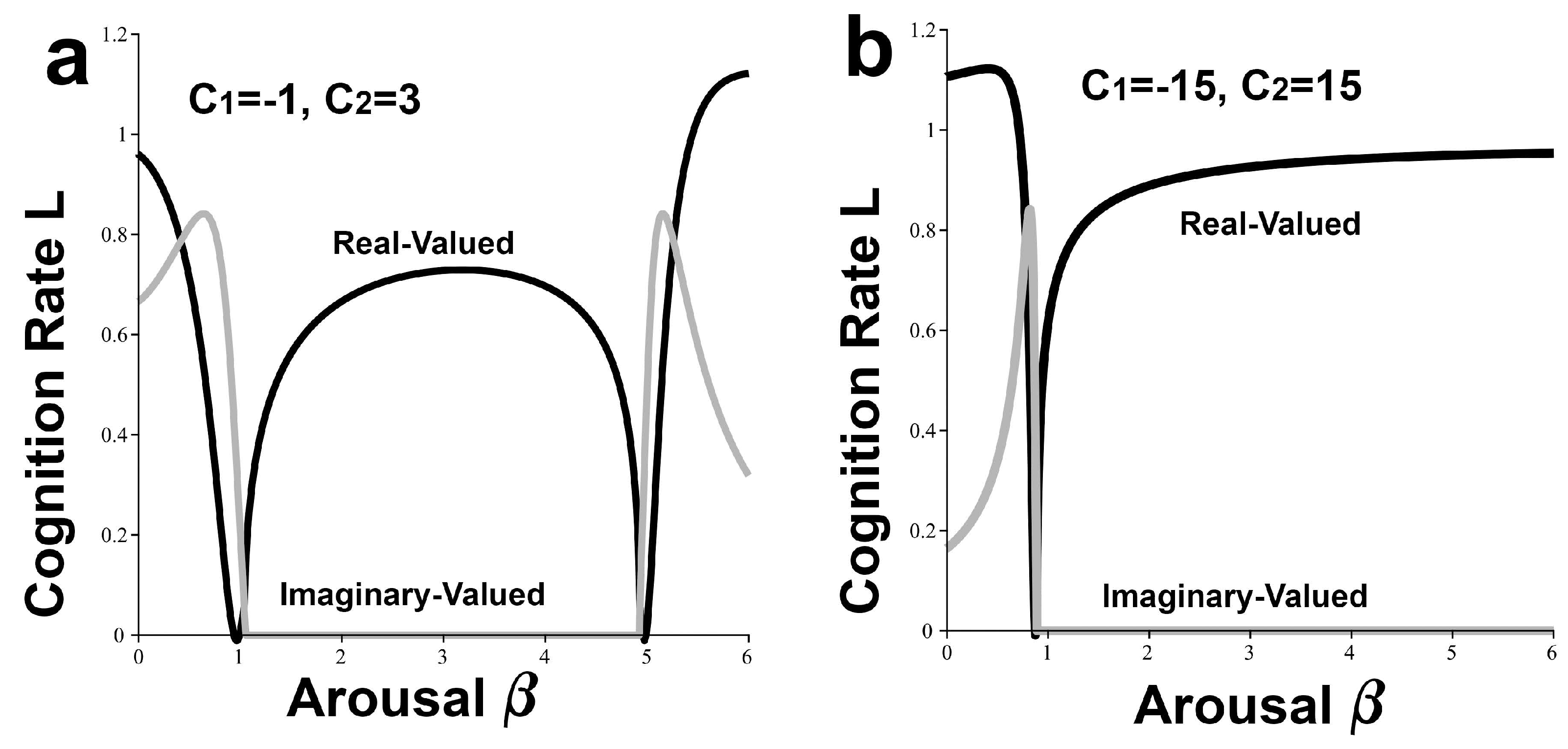
Plugging Equation (12) into Equations (9) and (12), and taking $R_0=1$ for the two sets of boundary conditions $C_1=-1,C_2=3$ and $C_1=-15,C_2=15$ produces Figure 2a,b. These replicate, respectively, the ‘hard’ and ‘easy’ versions of the Yerkes–Dodson effect [35,36], absent imposed ‘noise’, which requires another step. In Figure 2a, an inverted-U Yerkes–Dodson signal transduction is bracketed on the left and right by ‘hallucination’ [37] and ‘panic’ modes, for which the imaginary component is nonzero [38].

Introduction of ‘noise’ for the ‘hard’ problem of Figure 2a at the peak $\beta =3$ is via a new base stochastic differential equation in Z so that [39,40]

$$d{Z}_t=(\beta -\alpha Z_t)dt+\sigma Z_{t}d{B}_t$$

(13)

where the second term is an ‘ordinary’ volatility model in Brownian white noise $d{B}_t$ [22].

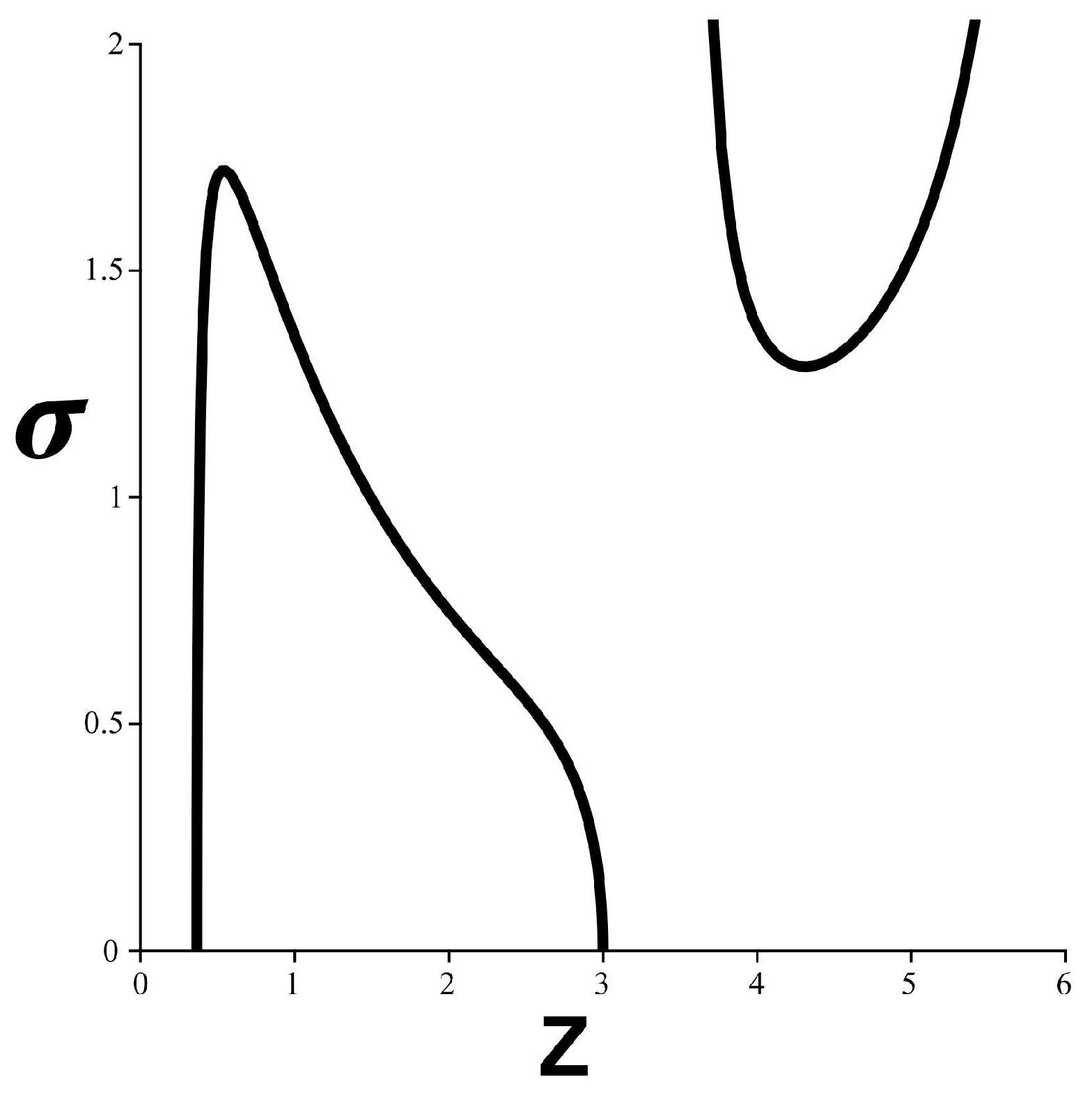
Here, we want to examine the equivalence class $\{Z,\sigma \}$ corresponding to the nonequilibrium steady state (nss) relation $<d{L}_t>=0$. This is carried out through the Itô Chain Rule [39,40], giving Figure 3.

At $\sigma =0$, the system starts out at the peak of Figure 2a, with Z declining smoothly as $\sigma$ increases until $\sigma \approx 1.3$, where a bifurcation instability transition becomes possible. This graph instantiates the synergism between fog and friction for this model.

6. The Cauchy Distribution

The Cauchy Distribution on the positive real line has the form

$$\rho (s,x)=\frac{2}{\pi }\left(\frac{s}{s^2+x^2}\right)$$

(14)

This distribution has indeterminate mean, variance, and kurtosis, indicating that it is indeed ‘fat-tailed’ in the sense of Taleb [21] and Derman et al. [22].

The relation $\rho (s,F/g)=g$, however, has the simple solution

$$g=\frac{1+\sqrt{1-{\pi }^2{F}^2}}{\pi s}$$

(15)

The cognition rate from Equation (5) is then

$$L=\frac{\mathrm{csgn}\left(\frac{1}{sg}\right)\pi -2arctan\left(\frac{R_0}{sg}\right)}{\pi \mathrm{csgn}\left(\frac{1}{sg}\right)}$$

(16)

where $\mathrm{csgn}\left(x\right)$ is the sign of x.

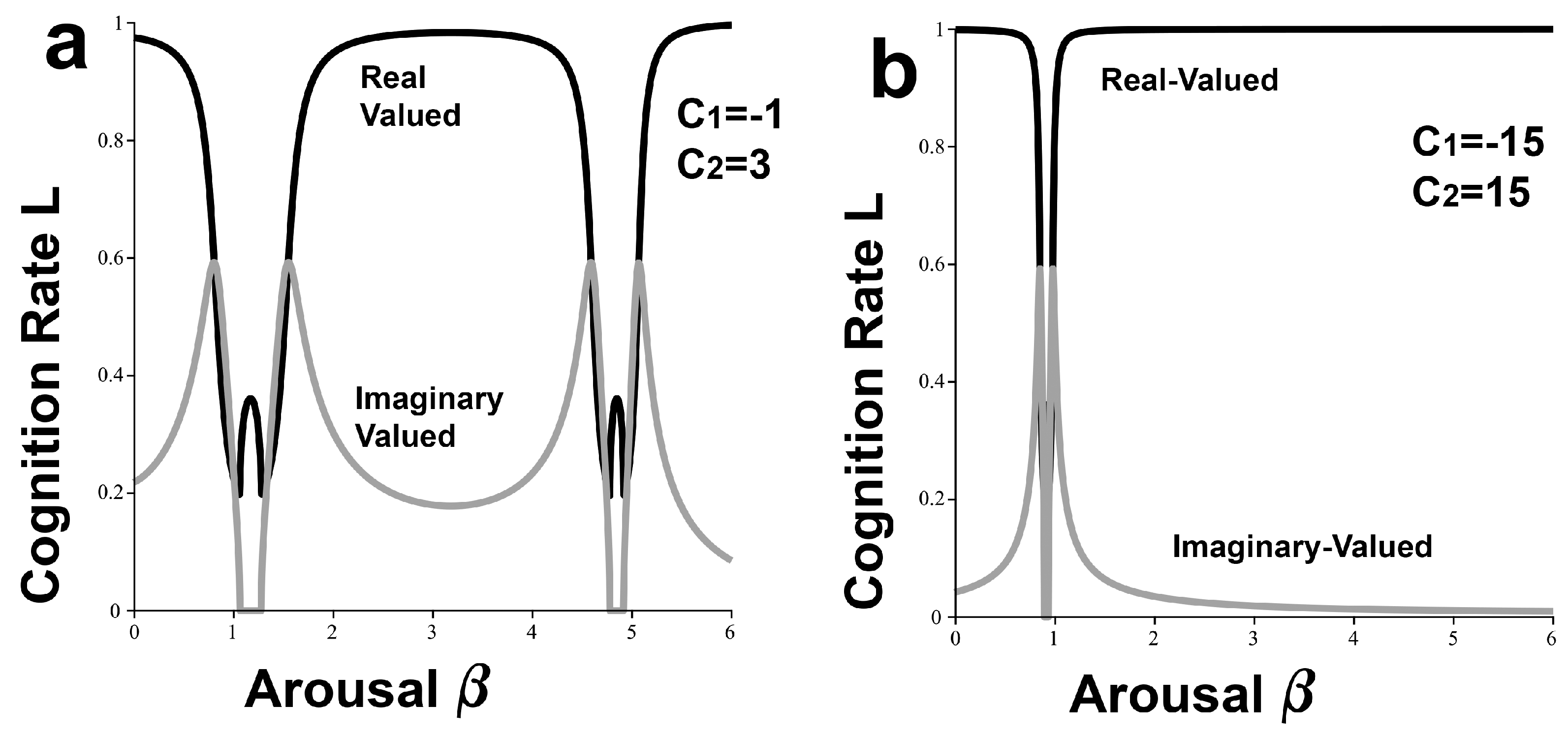
We use the base parameters of Figure 2 under the fog-and-friction model. That is, $\alpha =1,R_0=1$, with $\beta$ as the ‘arousal’. The two corresponeing boundary condition sets are $C_1=-1,C_2=3$ and $C_1=-15,C_2=15$. This leads to Figure 4a,b, the ‘hard’ and ‘easy’ Yerkes–Dodson models. Here, as opposed to Figure 2, the imaginary components are nonzero except over very narrow ranges, implying that a system driven by an underlying Cauchy Distribution will be far less stable than one characterized by the Exponential Distribution (again, Johnson [38]).

The stochastic analysis leading to Figure 3 is not warranted in this case.

It is not difficult to show similar results for the Lévy Distribution, which has similarly undefined mean, variance, and kurtosis.

7. Environmental Shadow Price and the Exponential Model

We next extend the remarks of Wallace and Fricchione [41]. Cognition, like evolution, it can be argued, operates on a fitness landscape constrained by circumstance and ‘riverbanks’ of culture and path-dependent historical trajectories that confine and circumscribe individual minds, as well as small group and institutional cognition. In a military setting, such a particular way-of-war is often represented as ‘doctrine’.

We further suppose that a group of cognitive entities at some scale, or an institution at larger scales, attempts to maximize an index of critical function across a multi-component system restricted by resource rates and by the need to respond collectively to environmental signals within both time and ‘energy’ constraints. As above, we take the rate at which essential resources indexed by Z can be delivered as

$$\partial Z_i/\partial t=f_i\left(Z_i\right)$$

(17)

The system is composed of $i=1,2,\dots ,m$ cooperating units that must be individually supplied with resources at rates $Z_i$ under overall constraints on resources and time as $Z={\sum }_i{Z}_i$ and $T={\sum }_i{T}_i$. We then attempt to optimize a critical scalar index of function, like cognition rates, across the full system, under these constraints.

Although more general approaches are possible [42], a simple Lagrangian optimization demonstrates the basic idea:

$$\begin{array}{c}\hfill \mathcal{L}\equiv \sum _i{L}_i+\lambda \left(Z-\sum _i{Z}_i\right)+\mu \left(T-\sum _i{T}_i\right)\\ \hfill \partial \mathcal{L}/\partial Z=\lambda ,\partial L_i/\partial Z_i=\lambda ,\partial L_i/\partial T_i=\mu \end{array}$$

(18)

under the condition that $\partial Z_i/\partial T_i=f_i\left(Z_i\right)$ from Equation (17).

In economic theory, $\lambda$ and $\mu$ are ‘shadow prices’ imposed on a system by environmental constraints [43,44].

Simple algebraic manipulation gives the important relation

$$d{Z}_i/d{T}_i=f_i\left(Z_i\right)=\frac{\mu }{\lambda }$$

(19)

We finesse matters by reconsidering the SDE arguments above, setting $d{Z}_i/dt=\mu /\lambda$ so that, under shadow price constraint or affordance, the fundamental SDE becomes

$$d{Z}_t^i=\frac{\mu }{\lambda }dt+{\sigma }_i{Q}_i\left(Z_t^i\right)d{B}_t$$

(20)

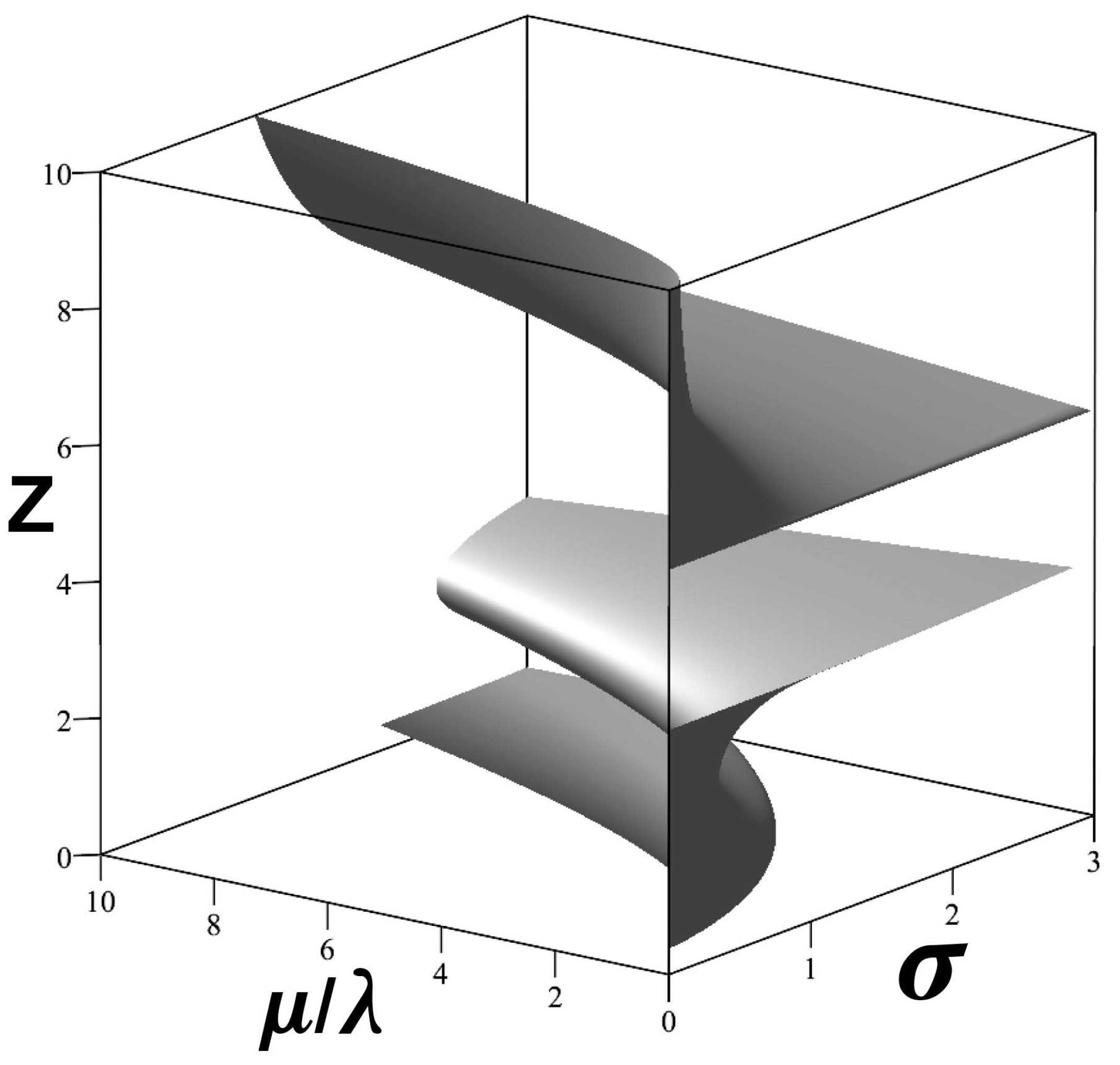
Setting Q(Z) = Z, and using the Itô Chain Rule to calculate the nonequilibrium steady state condition $<d{L}_t^i>=0$ for the Exponential model of Figure 2a allows for the calculation of a convoluted solution set $\{\sigma ,\mu /\lambda ,Z_i\}$ as shown in Figure 5. Certain combinations of shadow price ratio and ‘noise’ level will drive $Z_{nss}^i$ below any critical value, causing component i to fail.

Increasing ‘noise’ $\sigma$ can become synergistic with the global environmental shadow price ratio $\mu /\lambda$, where the numerator represents the time constraint and the denominator represents the resource rate constant. This will determine the nonequilibrium steady state resource rate available to level i—the rate $Z_{nss}^i$. The shadow price ratio can either buffer against or amplify the effects of ‘noise’ in determining the rate of resources available at level i.

In sum, the embedding, environmental shadow price ratio—selection pressure or affordance—can profoundly affect the regulation of individual component cognition across an entire interlinked hierarchical system.

8. Expanding the Formal Perspective

Again following Wallace and Fricchione [41], Equations (6) and (7) are only the first of a large class of possible regression models analogs. Dimensionally consistent extensions without cross-terms can be written as

$$\begin{array}{c}\hfill S\equiv -F\left(Z\right)+ZdF/dZ+\sum _{n=2}^{\infty }{ϵ}_n{Z}^n{d}^{n}F/d{Z}^n\\ \hfill \partial Z/\partial t=\mu dS/dZ+\sum _{n=2}^{\infty }{\mu }_n^{n-1}{d}^{n}S/d{Z}^n\end{array}$$

(21)

As Jackson et al. [45] put it,

The Legendre transform can be viewed as mapping the coefficients of one formal power series into the coefficients of another formal power series. Here, the term ‘formal’ does not express ‘mathematically nonrigorous’, as it often does in the physics literature. Instead, the term ‘formal power series’ is here a technical mathematical term, meaning a power series in indeterminates. Formal power series are not functions. A priori, formal power series merely obey the axioms of a ring and questions of convergence do not arise.

In contrast to physical models, the $ϵ$ and $\mu$ spectra—and possible series crossterms—raise fundamental empirical questions typical of all statistical models, analogous to fitting regression equations to observational or experimental data.

9. Some Tactical Observations

Rather remarkably, the expressions for cognition rate across one-parameter distributions depend only on a free energy index F that is driven by ‘arousal’, in a large sense, and on the detection threshold $R_0$.

The independence of the cognition rate from the one-dimensional ‘shape’ parameters is striking, although the functional forms for $L(F,R_0)$ differ markedly. ‘Maskirovka’ efforts, in these cases, can be aimed at affecting both the detection threshold—by continually reinforcing an opponent’s expectations—or by forcing a shift to an unfavorable underlying probability distribution on that opponent, for example, from a thin- to a fat-tailed distribution via burdens of widespread harassment by bombardment, armoured breakthrough, or partisan activity. Nonetheless, possible cognition rate robustness with regard to distribution ‘shape’ parameters is worth keeping in mind.

By contrast, under stress or selection pressure, healthy ‘natural’ systems may be able to more appropriately ‘tune’ across both the detection threshold and the underlying probability distribution itself. The converse, of course, would represent the onset of pathology.

10. Discussion

Organized conflict, while confined by the laws of physics—and, under what amounts to profound strategic incompetence, by WW I’s Lanchester equations [5,6,13]—is not a physical process per se. It is, rather, an extended exchange—ein Gespräch-über-Politik—between cognitive entities that have been shaped by path-dependent historical trajectories and longstanding cultural traditions.

Within such broad limits, however, cognition itself is confined by the necessity of duality, with an underlying information source constrained by the asymptotic limit theorems of information and control theories. This perspective permits the construction of a new class of probability models that may provide new statistical tools for the analysis of observational and experimental data associated with organized conflict and perhaps for the limited contribution to its management. Much more than this, for example, thoughts of a supremely competent General Staff Artificial Intelligence, borders on hallucination: cultural imperatives aside, organized conflict is not a game of Go, and the enemy always has a strong vote on the outcome [46,47].

Here, we have, in the generalized probability model of Equations (1)–(12), introduced the idea of a basic underlying probability distribution (BUPD) $\rho (c,x)$ characteristic of the given cognitive process under study, as possibly extended by the considerations of Section 8. In particular, we have emphasized the differences in dynamics and stability between thin-tailed and fat-tailed distributions, with the latter characterizing jump-diffusion phenomena. Indeed, a potential tactic in organized conflict then becomes the deliberate and systematic induction of such destabilizing jump-diffusions in an opponent’s BUPD. One thinks, for example, of concerted resistance and partisan attacks on Wehrmacht rail infrastructure in the immediate run-ups to the D-Day Normandy landings and Operation Bagration. These efforts were synergistic with Allied and Russian air superiority that further degraded timely Wehrmacht responses on both fronts.

The experiences of the USSR in Afghanistan and of the US in Korea after Inchon and in Vietnam, Iraq, and Afghanistan, of course, also come to mind.

Section 7 further explored a necessary parallel synergism between externally induced shadow price constraints of various origins and ‘noise’ in even for a thin-tailed BUPD.

Again and again, however, the conversion of probability models like those explored here into useful statistical tools for the study and limited management of organized conflict remains an arduous enterprise.

11. Mathematical Appendix

We briefly explore the necessary conditions for the independence of the cognition rate on the scale parameter for a distribution $\rho (s,x)$.

Recall that

$$\rho (s,F/g(s,F))={\int }_0^{\infty }\rho (s,R/g(s,F))dR=g(s,F)$$

(22)

The cognition rate is given as

$$\begin{array}{c}\hfill L\equiv \frac{{\int }_{R_0}^{\infty }\rho (s,R/g(s,F))dR}{{\int }_0^{\infty }\rho (s,R/g(s,F))dR}=\frac{1}{g(s,F)}{\int }_{R_0}^{\infty }\rho (s,R/g(s,F))dR\\ \hfill ={\int }_{R_0/g(s,F)}^{\infty }\rho (s,u)du=1-{\int }_0^{R_0/g(s,F)}\rho (s,u)du\end{array}$$

(23)

Taking the derivative of the last relation in Equation (23) with respect to the shape parameter s gives

$$\begin{array}{c}\hfill {\int }_{R_0/g(s,F)}^{\infty }\partial \rho (s,u)/\partial sdu+Q(R_0,s,F)=\\ \hfill -{\int }_0^{R_0/g(s,F)}\partial \rho (s,u)/\partial sdu+Q(R_0,s,F)\end{array}$$

(24)

where

$$Q(R_{0}s,F)=\frac{{\mathit{R}}_0\left(\frac{\partial }{\partial s}g\left(s,F\right)\right)\rho \left(s,\frac{{\mathit{R}}_0}{g\left(s,F\right)}\right)}{g{\left(s,F\right)}^2}$$

(25)

The complicated expressions $Q(R_0,s,F)$ cancel out, leaving the necessary condition

$${\int }_0^{\infty }\partial \rho (s,u)/\partial sdu=0$$

(26)

which is trivially satisfied for a probability distribution.