Efficient Newton-Type Solvers Based on for Finding the Solution of Nonlinear Algebraic Problems

Abstract

The purpose of this study is to improve the computational efficiency of solvers for nonlinear algebraic problems with simple roots. To this end, a multi-step solver based on Newton’s method is utilized. Divided difference operators are applied at two substeps in various forms to enhance the convergence speed and, consequently, the solver’s efficiency index. Attraction basins for the proposed solvers and their competitors are presented, demonstrating that the proposed solvers exhibit large attraction basins in the scalar case while maintaining high convergence rates. Theoretical findings are supported by numerical experiments.

1. Background and Introductory Notes

Nonlinear equations frequently arise across numerous disciplines within science and engineering, and they play a significant part in the field of applied mathematics. Due to the inherent complexity of these equations, obtaining exact analytical solutions is typically challenging or unattainable. As a result, numerical iterative techniques are widely utilized to compute approximate solutions [1].

The impetus for this manuscript is to develop a rapid iteration method that enhances both efficacy and accuracy to solve nonlinear collections of equations; see the pioneer discussions in the works [2,3]. By avoiding the necessity for second Fréchet derivatives, our approach attempts to mitigate the complexity and efficiency of the available methodologies, hence contributing to advancements in the field of computational mathematics. The initial aim is to provide a high-rate solver for tackling nonlinear sets, accommodating both real and complex simple roots. Then, the aim is to improve calculational efficacy via decreasing the frequency of matrix inverses and the number of functional evaluations, aligning with the foundational frameworks of computational mathematics.

We take into consideration a class of nonlinear algebraic equations presented in ([4] Chapter 5):

$$L\left(z\right)=0,$$

(1)

wherein $L\left(z\right)={(g_1\left(z\right),g_2\left(z\right),\dots ,g_{\upsilon }\left(z\right))}^T$ and each $g_i\left(z\right)$, $1\le i\le \upsilon$ represents a coordinate function. We assume that $L\left(z\right)$ is sufficiently differentiable inside an open and convex domain $D\subseteq {\mathbb{R}}^{\upsilon }$. Initially, we investigate several foundational iterative methods designed to solve the Equation (1). A widely recognized approach is Newton’s method (NM2), which is articulated as follows [5]:

$$\left\{\begin{array}{c}{L}^{\prime }\left({\sigma }^{\left(\varrho \right)}\right){\delta }^{\left(\varrho \right)}=-L\left({\sigma }^{\left(\varrho \right)}\right),\varrho =0,1,2,\dots ,\hfill \\ {\sigma }^{(\varrho +1)}={\delta }^{\left(\varrho \right)}+{\sigma }^{\left(\varrho \right)}.\hfill \end{array}\right.$$

(2)

This method reaches the quadratical rate, contingent upon the initial value ${\sigma }^{\left(0\right)}$ being enough close to the simple zero. To circumvent some limitations corresponding to NM2, alternative solvers [6], such as Steffensen’s method (SM2), have been developed, which do not require derivative computations [7]. The SM2 for addressing nonlinear systems is defined [8]

$$\left\{\begin{array}{c}{\lambda }^{\left(\varrho \right)}=L\left({\sigma }^{\left(\varrho \right)}\right)+{\sigma }^{\left(\varrho \right)},\hfill \\ {\sigma }^{(\varrho +1)}=-{[{\sigma }^{\left(\varrho \right)},{\lambda }^{\left(\varrho \right)},L]}^{-1}L\left({\sigma }^{\left(\varrho \right)}\right)+{\sigma }^{\left(\varrho \right)},\varrho =0,1,2,\dots ,\hfill \end{array}\right.$$

(3)

which employs the divided difference operator (DDO). For high-dimensional points $\tau$ and y, the first-order DDO of L is defined as follows ($1\le i,j\le m$):

$${[\tau ,y;L]}_{i,j}={\displaystyle \frac{-L_i({\tau }_1,\dots ,{\tau }_{j-1},y_j,\dots ,y_m)+L_i({\tau }_1,\dots ,{\tau }_j,y_{j+1},\dots ,y_m)}{-y_j+{\tau }_j}}.$$

(4)

In a more general context, the DDO for L in ${\mathbb{R}}^m$ can be formulated as [8]

$$[·,·;L]:D\subset {\mathbb{R}}^m\times {\mathbb{R}}^m\to \mathcal{L}\left({\mathbb{R}}^m\right),$$

(5)

which satisfies the relationship $[y,\tau ;L](-\tau +y)=L\left(y\right)-L\left(\tau \right)$, $\forall \tau ,y\in D.$ By letting $h=y-\tau$, the first-order DDO is written via the following [9]:

$$[\tau +h,\tau ;L]={\int }_0^1{L}^{\prime }(\tau +th)dt.$$

(6)

However, the definitions provided in (4)–(6) primarily result in dense matrices for representing the DDO, which limits the applicability of the SM2 to solve (1) effectively. Traub introduced an enhancement to NM2 that achieves local cubic convergence [10] (TM):

$$\left\{\begin{array}{c}{\gamma }^{\left(\varrho \right)}={\sigma }^{\left(\varrho \right)}-L^{\prime }{\left({\sigma }^{\left(\varrho \right)}\right)}^{-1}L\left({\sigma }^{\left(\varrho \right)}\right),\hfill \\ {\sigma }^{(\varrho +1)}={\gamma }^{\left(\varrho \right)}-L^{\prime }{\left({\sigma }^{\left(\varrho \right)}\right)}^{-1}L\left({\gamma }^{\left(\varrho \right)}\right).\hfill \end{array}\right.$$

(7)

Another prominent and efficient technique to solve (1) is the quartically convergent Jarratt method [11,12], given as follows (JM4):

$$\left\{\begin{array}{c}{y}^{\left(\varrho \right)}={\sigma }^{\left(\varrho \right)}-{\displaystyle \frac{2}{3}}{L}^{\prime }{\left({\sigma }^{\left(\varrho \right)}\right)}^{-1}L\left({\sigma }^{\left(\varrho \right)}\right),\hfill \\ {\sigma }^{(\varrho +1)}={\sigma }^{\left(\varrho \right)}-{\displaystyle \frac{1}{2}}{(3L^{\prime }\left(y^{\left(\varrho \right)}\right)-L^{\prime }\left({\sigma }^{\left(\varrho \right)}\right))}^{-1}\hfill \\ ·(3L^{\prime }\left(y^{\left(\varrho \right)}\right)+L^{\prime }\left({\sigma }^{\left(\varrho \right)}\right))L^{\prime }{\left({\sigma }^{\left(\varrho \right)}\right)}^{-1}L\left({\sigma }^{\left(\varrho \right)}\right).\hfill \end{array}\right.$$

(8)

In an effort to refine both (7) and (8), the authors of [13] have proposed a three-step sixth-rate solver that eliminates the necessity of computing DDO and second-order Fréchet derivatives to solve (1) as follows (MSM):

$$\left\{\begin{array}{c}{\eta }^{\left(\varrho \right)}=L^{\prime }{\left({\sigma }^{\left(\varrho \right)}\right)}^{-1}L\left({\sigma }^{\left(\varrho \right)}\right),\hfill \\ {\xi }^{\left(\varrho \right)}={\sigma }^{\left(\varrho \right)}-{\displaystyle \frac{2}{3}}{\eta }^{\left(\varrho \right)},\hfill \\ {\gamma }^{\left(\varrho \right)}={\sigma }^{\left(\varrho \right)}-\left[{\displaystyle \frac{23}{8}}I-3L^{\prime }{\left({\sigma }^{\left(\varrho \right)}\right)}^{-1}{L}^{\prime }\left({\xi }^{\left(\varrho \right)}\right)+{\displaystyle \frac{9}{8}}{\left(L^{\prime }{\left({\sigma }^{\left(\varrho \right)}\right)}^{-1}{L}^{\prime }\left({\xi }^{\left(\varrho \right)}\right)\right)}^2\right]{\eta }^{\left(\varrho \right)},\hfill \\ {\sigma }^{(\varrho +1)}={\gamma }^{\left(\varrho \right)}-\left[{\displaystyle \frac{5}{2}}I-{\displaystyle \frac{3}{2}}{L}^{\prime }{\left({\sigma }^{\left(\varrho \right)}\right)}^{-1}{L}^{\prime }\left({\xi }^{\left(\varrho \right)}\right)\right]L^{\prime }{\left({\sigma }^{\left(\varrho \right)}\right)}^{-1}L\left({\gamma }^{\left(\varrho \right)}\right).\hfill \end{array}\right.$$

(9)

These solvers are distinguished not only by their straightforward implementation but also by their computational efficiency. For a thorough overview of this subject, please refer to [14,15].

This article introduces two multi-step higher-order solvers aimed at resolving (1), specifically proposing fourth- and fifth-order iterative techniques for computing simple zeros. These solvers circumvent the need for computing the second Fréchet differentiation.

This manuscript is structured as follows:

• Section 2 provides a discussion of multi-step schemes comprising three substeps to reach fast convergence, while utilizing a minimal number of LU decompositions (also known as lower–upper (LU) decomposition).
• Section 3 includes an error analysis and assesses convergence rates.
• The dynamic characteristics of the proposed schemes in contrast to those of the available solvers are compared in Section 4.
• Additionally, Section 5 applies the proposed method to several test problems.
• Finally, Section 6 concludes with findings and outlines future research directions.

2. A New Procedure

We propose an enhanced iterative scheme that builds upon the pioneer methods discussed in Section 1, incorporating multiple steps while maintaining a fixed Jacobian, as follows (PM1):

$$\left\{\begin{array}{c}{y}^{\left(\varrho \right)}={\sigma }^{\left(\varrho \right)}-L^{\prime }{\left({\sigma }^{\left(\varrho \right)}\right)}^{-1}L\left({\sigma }^{\left(\varrho \right)}\right),\hfill \\ {\xi }^{\left(\varrho \right)}=y^{\left(\varrho \right)}-{\left[{\sigma }^{\left(\varrho \right)},y^{\left(\varrho \right)};L\right]}^{-1}L\left(y^{\left(\varrho \right)}\right),\hfill \\ {\sigma }^{(\varrho +1)}={\xi }^{\left(\varrho \right)}-{\left[{\sigma }^{\left(\varrho \right)},y^{\left(\varrho \right)};L\right]}^{-1}L\left({\xi }^{\left(\varrho \right)}\right).\hfill \end{array}\right.$$

(10)

The DDO during the second and third substeps is intentionally held constant to maximize convergence enhancement; see the discussions in [16,17]. However, to boost the convergence, we may use an updated node value in the DDO of the third substep, which would lead to a higher convergence speed as follows (PM2):

$$\left\{\begin{array}{c}{y}^{\left(\varrho \right)}={\sigma }^{\left(\varrho \right)}-L^{\prime }{\left({\sigma }^{\left(\varrho \right)}\right)}^{-1}L\left({\sigma }^{\left(\varrho \right)}\right),\hfill \\ {\xi }^{\left(\varrho \right)}=y^{\left(\varrho \right)}-{\left[{\sigma }^{\left(\varrho \right)},y^{\left(\varrho \right)};L\right]}^{-1}L\left(y^{\left(\varrho \right)}\right),\hfill \\ {\sigma }^{(\varrho +1)}={\xi }^{\left(\varrho \right)}-{\left[{\xi }^{\left(\varrho \right)},y^{\left(\varrho \right)};L\right]}^{-1}L\left({\xi }^{\left(\varrho \right)}\right).\hfill \end{array}\right.$$

(11)

Furthermore, in practical implementations, matrix inversion is to be avoided. Hence, we employ LU decompositions for linear systems. Thus, we attain the following four linear algebraic equations in the process of handling PM1 or PM2 to calculate the simple root of a nonlinear algebraic problem (1):

$$\left\{\begin{array}{c}{L}^{\prime }\left({\sigma }^{\left(\varrho \right)}\right)Y^{\left(\varrho \right)}=L\left({\sigma }^{\left(\varrho \right)}\right),\hfill \\ \left[{\sigma }^{\left(\varrho \right)},y^{\left(\varrho \right)};L\right]M^{\left(\varrho \right)}=L\left(y^{\left(\varrho \right)}\right),\hfill \\ \left[{\sigma }^{\left(\varrho \right)},y^{\left(\varrho \right)};L\right]N^{\left(\varrho \right)}=L\left({\xi }^{\left(\varrho \right)}\right),\hfill \\ \left[{\xi }^{\left(\varrho \right)},y^{\left(\varrho \right)};L\right]P^{\left(\varrho \right)}=L\left({\xi }^{\left(\varrho \right)}\right),\hfill \end{array}\right.$$

(12)

Then, the iterative expressions PM1 and PM2 can be simply reformulated in implementations as follows:

$$\left\{\begin{array}{c}{y}^{\left(\varrho \right)}={\sigma }^{\left(\varrho \right)}-Y^{\left(\varrho \right)},\hfill \\ {\xi }^{\left(\varrho \right)}=y^{\left(\varrho \right)}-M^{\left(\varrho \right)},\hfill \\ {\sigma }^{(\varrho +1)}={\xi }^{\left(\varrho \right)}-N^{\left(\varrho \right)},\hfill \end{array}\right.$$

(13)

and

$$\left\{\begin{array}{c}{y}^{\left(\varrho \right)}={\sigma }^{\left(\varrho \right)}-Y^{\left(\varrho \right)},\hfill \\ {\xi }^{\left(\varrho \right)}=y^{\left(\varrho \right)}-M^{\left(\varrho \right)},\hfill \\ {\sigma }^{(\varrho +1)}={\xi }^{\left(\varrho \right)}-P^{\left(\varrho \right)}.\hfill \end{array}\right.$$

(14)

We adhered to a fundamental principle in computational mathematics which asserts that the true evaluation of numerical algorithms is based on computational efficiency. This efficiency was directly related to the quality of the method and inversely related to its calculational cost. The quality of a method has was measured by its convergence rate and structural properties, while its calculational cost referred to the amount of work required for function evaluations, derivatives, and LU decompositions throughout the process. With these considerations in mind, we provided fourth- and fifth-order methods PM1 and PM2 based on different DDOs (of the first order).

While several sixth- and seventh-order methods exist in the literature [13,16] that perform well for resolving collections of nonlinear equations, our objective here is to demonstrate that effective fourth- and fifth-rate schemes can also be developed. By strategically freezing the DDO or applying it at suitable stages, the convergence domain may be extended, as will be shown in Section 4.

This approach is novel in the literature for nonlinear systems, focusing primarily on expanding the attraction basins (as will be seen in Section 4). In contrast, other frozen-type schemes tend to lose their broad convergence domain due to the application of multiple frozen Jacobians. The process of the proposed solvers are summarized in Algorithm 1 and the flowchart of Figure 1.

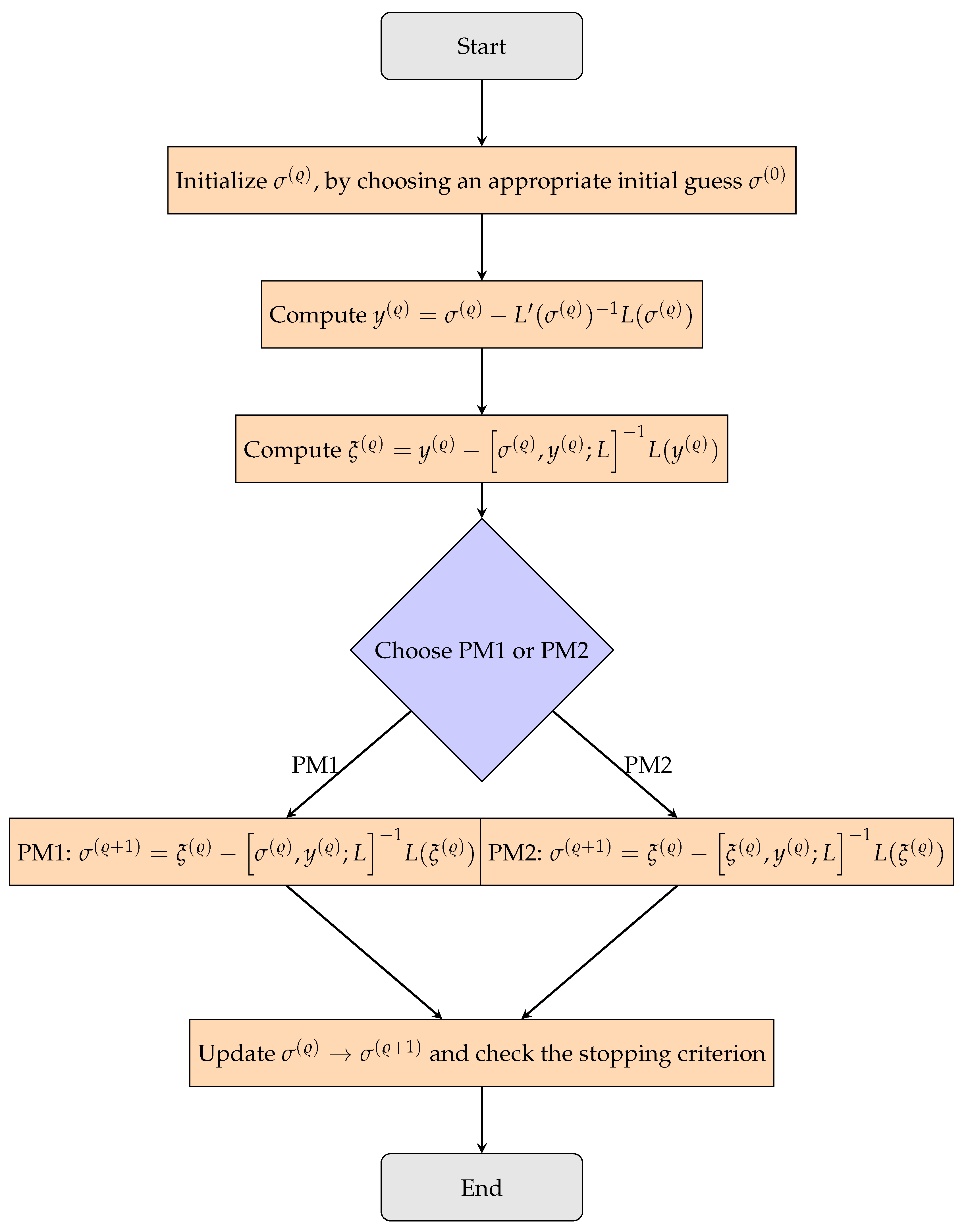
Algorithm 1 The algorithmic format of the multi-step iterative schemes (PM1 and PM2).

1: Input: Initial guess ${\sigma }^{\left(0\right)}$, tolerance $ϵ$ and a stopping termination, or maximum iterations ${\sigma }_{\max }$  2: Output: Approximate solution ${\sigma }^{(\varrho +1)}$  3: Initialize $\varrho \leftarrow 0$  4: while $∥L\left({\sigma }^{\left(\varrho \right)}\right)∥>ϵ$ and/or $\varrho <{\sigma }_{\max }$ do  5:    Compute $y^{\left(\varrho \right)}={\sigma }^{\left(\varrho \right)}-L^{\prime }{\left({\sigma }^{\left(\varrho \right)}\right)}^{-1}L\left({\sigma }^{\left(\varrho \right)}\right)$ by using LU factorization to avoid the matrix inversion  6:    Compute ${\xi }^{\left(\varrho \right)}=y^{\left(\varrho \right)}-{\left[{\sigma }^{\left(\varrho \right)},y^{\left(\varrho \right)};L\right]}^{-1}L\left(y^{\left(\varrho \right)}\right)$ by using LU factorization to avoid the matrix inversion  7:    if using PM1 then  8:      Update ${\sigma }^{(\varrho +1)}={\xi }^{\left(\varrho \right)}-{\left[{\sigma }^{\left(\varrho \right)},y^{\left(\varrho \right)};L\right]}^{-1}L\left({\xi }^{\left(\varrho \right)}\right)$ and use the LU factorziation obtained in Line 6 to proceed  9:    else if using PM2 then 10:      Update ${\sigma }^{(\varrho +1)}={\xi }^{\left(\varrho \right)}-{\left[{\xi }^{\left(\varrho \right)},y^{\left(\varrho \right)};L\right]}^{-1}L\left({\xi }^{\left(\varrho \right)}\right)$ by using a new LU factorization to avoid the matrix inversion 11:    end if 12:    $\varrho \leftarrow \varrho +1$ 13: end while 14: Return ${\sigma }^{(\varrho +1)}$

3. Rates for Convergence

In this section, we provide a rigorous theoretical analysis of the convergence rate for the iterative schemes (13)–(14). Before presenting the primary theoretical results concerning convergence, we first introduce the $\upsilon$-dimensional Taylor expansion.

The convergence rates of the memoryless iterations PM1 and PM2 are established using $\upsilon$-dimensional Taylor expansions. Let ${\mathrm{er}}^{\left(\varrho \right)}={\sigma }^{\left(\varrho \right)}-\beta$ represent the error at the $\varrho$-th iteration. As discussed in [18],

$${\mathrm{er}}^{(\varrho +1)}=\left(F\right){\mathrm{er}}^{{\left(\varrho \right)}^p}+\mathcal{O}\left({\mathrm{er}}^{{\left(\varrho \right)}^{p+1}}\right).$$

(15)

The derived error equation indicates that F possesses the characteristics of a p-linear function, wherein $F\in \mathcal{L}({\mathbb{R}}^{\upsilon },{\mathbb{R}}^{\upsilon },\dots ,{\mathbb{R}}^{\upsilon })$ and p is the convergence order. In addition, one obtains

$${\mathrm{er}}^{{\left(\varrho \right)}^p}=(\underset{p\mathrm{terms}}{\underbrace{{\mathrm{er}}^{\left(\varrho \right)},{\mathrm{er}}^{\left(\varrho \right)},\dots ,{\mathrm{er}}^{\left(\varrho \right)}}}).$$

(16)

Let $L:D\subseteq {\mathbb{R}}^{\upsilon }\to {\mathbb{R}}^{\upsilon }$ be assumed to possess sufficient differentiability in the Fréchet sense over D. As established in [11], the m-th differentiation of L at $u\in {\mathbb{R}}^{\upsilon }$ for $m\ge 1$ is defined as an m-linear function, namely,

$$L^{\left(m\right)}\left(u\right):{\mathbb{R}}^{\upsilon }\times \cdots \times {\mathbb{R}}^{\upsilon }\to {\mathbb{R}}^{\upsilon },$$

(17)

so that $L^{\left(m\right)}\left(u\right)(v_1,\dots ,v_m)\in {\mathbb{R}}^{\upsilon }$. For $\beta +h\in {\mathbb{R}}^{\upsilon }$ situated in the neighborhood of the zero $\beta$ of (1), the Taylor series is capable of being expressed by the following [11]:

$$L(\beta +h)=L^{\prime }\left(\beta \right)\left[h+\sum _{m=2}^{p-1}{\Theta }_m{h}^m\right]+\mathcal{O}\left(h^p\right),$$

(18)

where

$${\Theta }_m={\displaystyle \frac{1}{m!}}{\left[L^{\prime }\left(\beta \right)\right]}^{-1}{L}^{\left(m\right)}\left(\beta \right),m\ge 2.$$

(19)

It follows that ${\Theta }_m{h}^m\in {\mathbb{R}}^{\upsilon }$ and ${\left[L^{\prime }\left(\beta \right)\right]}^{-1}\in \mathcal{L}\left({\mathbb{R}}^{\upsilon }\right)$. Moreover, for $L^{\prime }(·)$, we obtain

$$L^{\prime }(\beta +h)=L^{\prime }\left(\beta \right)\left[I+\sum _{m=2}^{p-1}m{\Theta }_m{h}^{m-1}\right]+\mathcal{O}\left(h^p\right),$$

(20)

whereas I gives the identity matrix. Also, $m{\Theta }_m{h}^{m-1}\in \mathcal{L}\left({\mathbb{R}}^{\upsilon }\right)$.

Theorem 1.

In (1), let $L:D\subseteq {\mathbb{R}}^{\upsilon }\to {\mathbb{R}}^{\upsilon }$ possess sufficient Fréchet differentiability at each point within D and $L\left(\beta \right)=0$ at $\beta \in {\mathbb{R}}^{\upsilon }$. Also, assume $L^{\prime }\left(z\right)$ is smooth and invertible at β. Next, ${\left\{{\sigma }^{\left(\varrho \right)}\right\}}_{\varrho \ge 0}$ produced by PM1 converges to β with a local fourth convergence order.

Proof. 

To establish the rate of convergence, using (18) and (20), the following approach is considered to obtain

$$L\left({\sigma }^{\left(\varrho \right)}\right)=L^{\prime }\left(\beta \right)\left[{\mathrm{er}}^{\left(\varrho \right)}+{\Theta }_2{{\mathrm{er}}^{\left(\varrho \right)}}^2+{\Theta }_3{{\mathrm{er}}^{\left(\varrho \right)}}^3+{\Theta }_4{{\mathrm{er}}^{\left(\varrho \right)}}^4\right]+\mathcal{O}\left({{\mathrm{er}}^{\left(\varrho \right)}}^5\right),$$

(21)

and

$$L^{\prime }\left({\sigma }^{\left(\varrho \right)}\right)=L^{\prime }\left(\beta \right)\left[I+2{\Theta }_2{\mathrm{er}}^{\left(\varrho \right)}+3{\Theta }_3{{\mathrm{er}}^{\left(\varrho \right)}}^2+4{\Theta }_4{{\mathrm{er}}^{\left(\varrho \right)}}^3\right]+\mathcal{O}\left({{\mathrm{er}}^{\left(\varrho \right)}}^4\right),$$

(22)

where ${\Theta }_i={\displaystyle \frac{1}{i!}}{\left[L^{\prime }\left(\beta \right)\right]}^{-1}{L}^{\left(i\right)}\left(\beta \right)$ for $i\ge 2$, and ${\mathrm{er}}^{\left(\varrho \right)}={\sigma }^{\left(\varrho \right)}-\beta$. From (21) and (22), we derive the following:

$$y^{\left(\varrho \right)}=\beta +{\displaystyle \frac{1}{3}}{\mathrm{er}}^{\left(\varrho \right)}+{\displaystyle \frac{2}{3}}{\Theta }_2{{\mathrm{er}}^{\left(\varrho \right)}}^2+\mathcal{O}\left({{\mathrm{er}}^{\left(\varrho \right)}}^3\right).$$

(23)

For the DDO matrix $\left[{\sigma }^{\left(\varrho \right)},y^{\left(\varrho \right)};L\right]$, we compute the Taylor expansion similarly to finally obtain the following error at the end of the second substep of PM1:

$$\begin{array}{ccc}\hfill {\xi }^{\left(\varrho \right)}-\beta & =& \left({\Theta }_2^2\right){{\mathrm{er}}^{\left(\varrho \right)}}^3+\left(-3{\Theta }_2^3+3{\Theta }_3{\Theta }_2\right){{\mathrm{er}}^{\left(\varrho \right)}}^4+\mathcal{O}\left({{\mathrm{er}}^{\left(\varrho \right)}}^5\right).\hfill \end{array}$$

(24)

We avoid providing them here for the sake of brevity and clarity. Similarly, we have the following:

$$\begin{array}{cc}\hfill L\left({\xi }^{\left(\varrho \right)}\right)=& L^{\prime }\left(\beta \right)[{\Theta }_3{{\mathrm{er}}^{\left(\varrho \right)}}^3+{\Theta }_4{{\mathrm{er}}^{\left(\varrho \right)}}^4]+\mathcal{O}\left({{\mathrm{er}}^{\left(\varrho \right)}}^5\right).\end{array}$$

(25)

Employing (24) and (25) in the third substep of PM1, we derive

$${\mathrm{er}}^{(\varrho +1)}=\left({\Theta }_2^2\right){{\mathrm{er}}^{\left(\varrho \right)}}^4+\mathcal{O}\left({{\mathrm{er}}^{\left(\varrho \right)}}^5\right),$$

(26)

showcasing a fourth-order convergence rate, while necessitating only two LU decompositions per iteration cycle. This concludes the proof.    □

Theorem 2.

In (1), consider that $L:D\subseteq {\mathbb{R}}^{\upsilon }\to {\mathbb{R}}^{\upsilon }$ is sufficiently Fréchet-differentiable at every point in D, with $L\left(\beta \right)=0$ for some of $\beta \in {\mathbb{R}}^{\upsilon }$. Furthermore, assume that $L^{\prime }\left(z\right)$ is continuous and invertible at β. Under these conditions, the sequence ${\left\{{\sigma }^{\left(\varrho \right)}\right\}}_{\varrho \ge 0}$ generated by PM2 converges locally to β with a fifth-order convergence rate.

Proof. 

The proof pursues the path of proof in Theorem 1. Accordingly, we provide only its ultimate error equation,

$${\mathrm{er}}^{(\varrho +1)}=\left({\Theta }_2^3\right){{\mathrm{er}}^{\left(\varrho \right)}}^5+\mathcal{O}\left({{\mathrm{er}}^{\left(\varrho \right)}}^6\right),$$

(27)

illustrating a fourth-order rate of convergence, while necessitating three LU decompositions per iteration. This completes the proof.    □

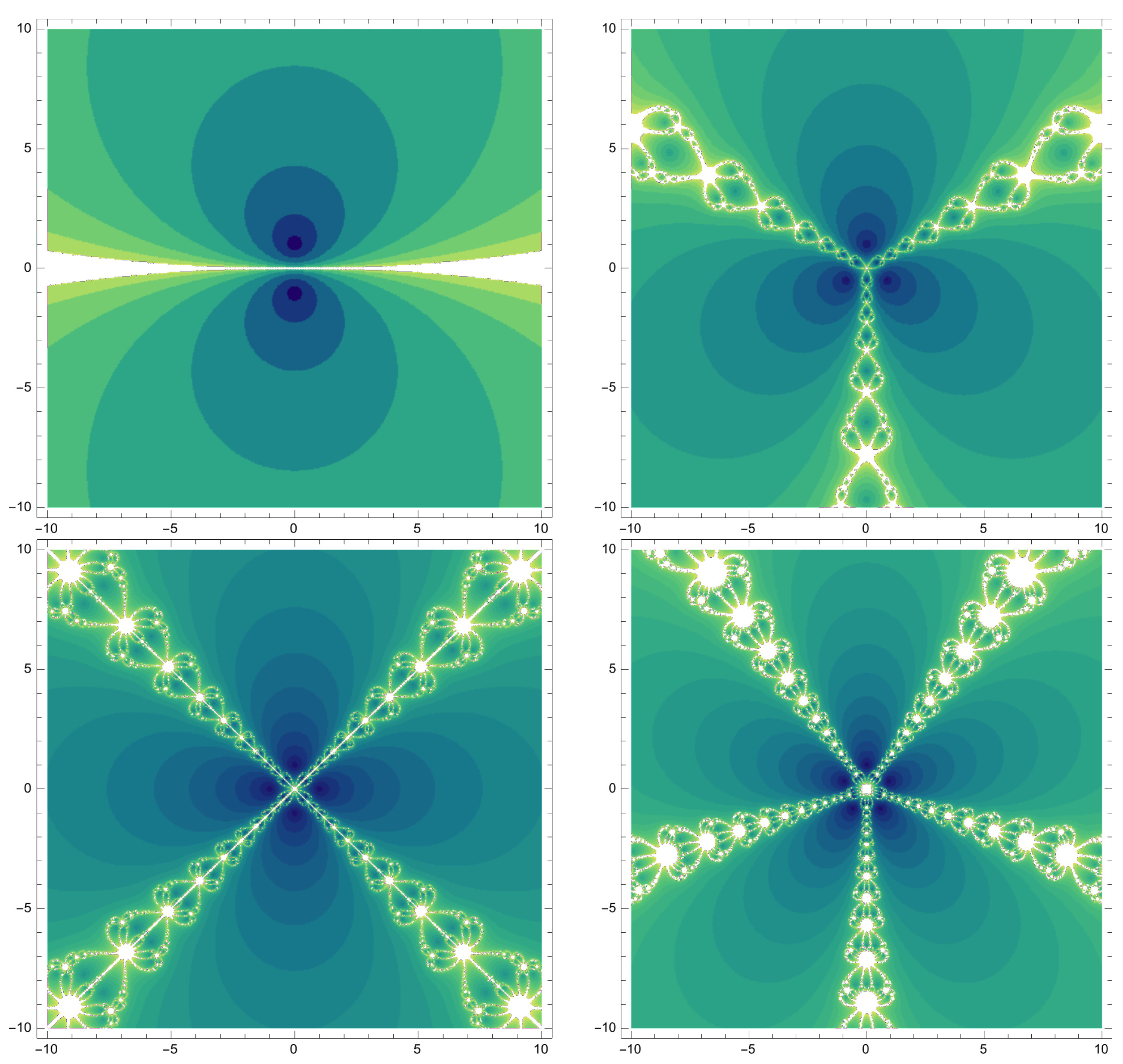
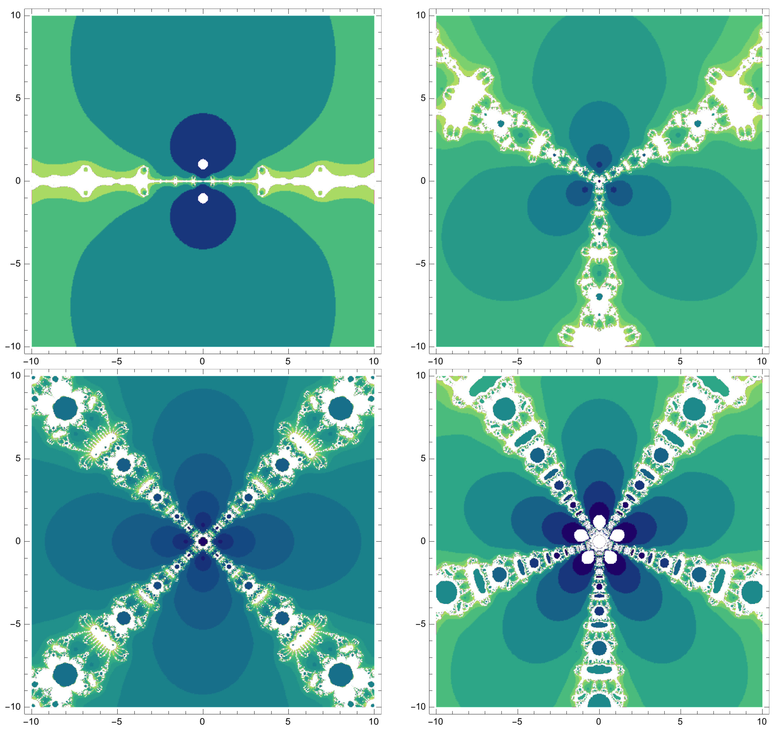
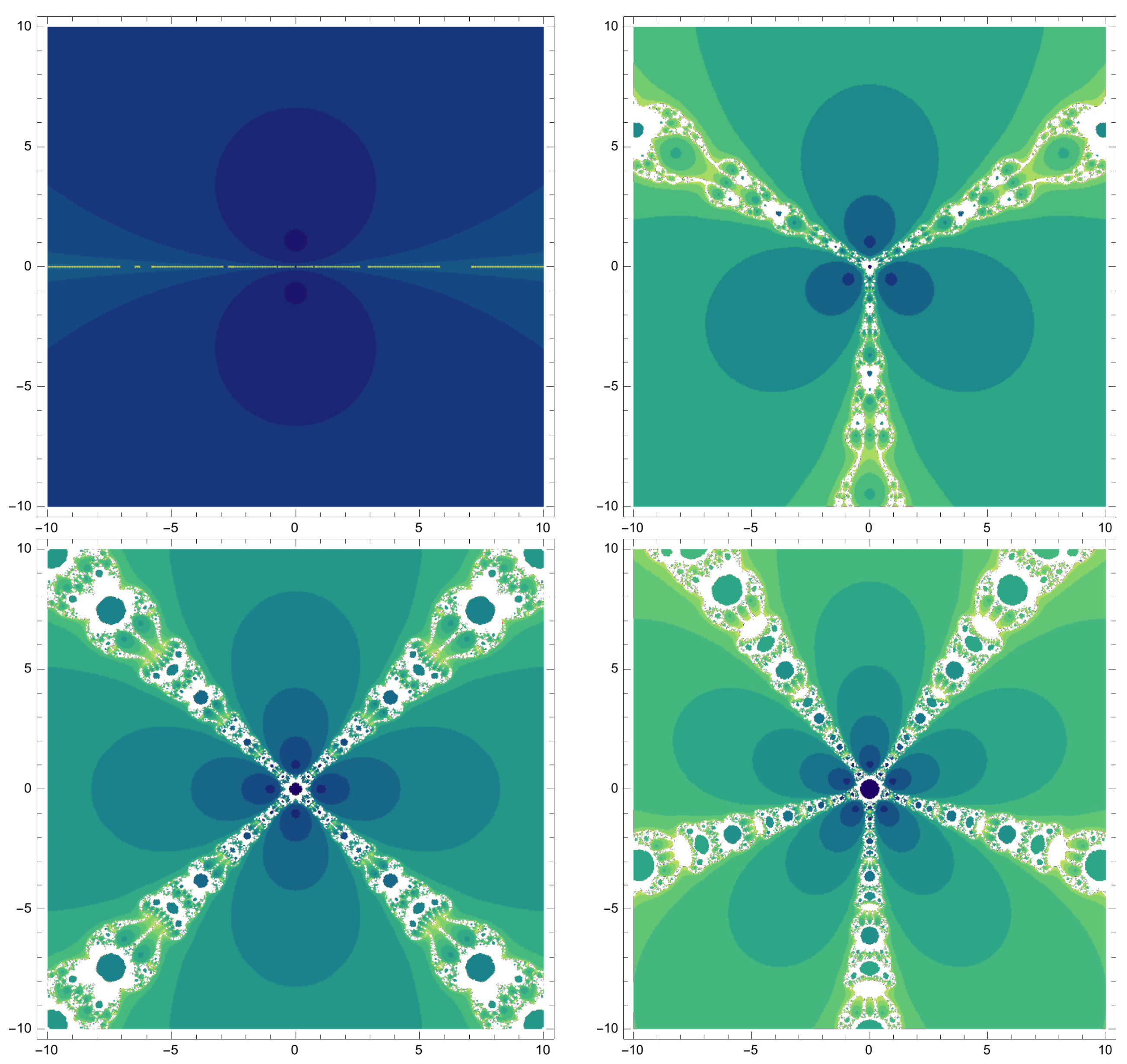
4. Dynamical Behavior

Without compromising generality, for the one variable scenario, the iterative schemes PM1 and PM2 emphasize the significance of illustrating the basin of attractions for iteration solvers applied to polynomial problems of varying degrees within the field of complex numbers [19]. This is particularly valuable in shading the plots via the required number of iterates to attain convergence. In the complex plane, distinct roots of a polynomial are associated with different areas of attraction. By visualizing such fractal-like basins, we can delineate the areas where starting approximations tend to specific zeros. The boundaries between these basins typically exhibit fractal characteristics, presenting a complex and intricate structure that is challenging to predict. As the polynomial degree increases, these boundaries become even more convoluted, making such visualizations instrumental in comprehending how polynomial complexity influences the convergence behavior of iterative methods.

Moreover, shading the plots according to the quantity of iterates necessary for convergence provides learning insights into the effectiveness of the scheme. Areas in which the method exhibits fast convergence can be regarded as zones of higher stability or greater computational efficiency, while regions needing more iterates (or those that fail to converge) indicate potential inefficiencies or instabilities. We included such discussions in Figure 2, Figure 3, Figure 4 and Figure 5, depicting the domain $[-10,10]\times [-10,10]$ with a maximum number of iterates set to 150 and a tolerance level of ${10}^{-3}$ for the residual as the stop termination. Four different solvers, PM1, PM2, JM4 and NM2, were compared.

In Figure 2, Figure 3, Figure 4 and Figure 5, the darkest color indicates the fewest number of iterations. In this way, it not necessary to write down the number of iterations in different tables since the shading of the colors indicates this procedure. The white-like areas show divergences or requiring many number of iterations to converge.

For the points on the boundaries of the regions in Figure 2, Figure 3, Figure 4 and Figure 5, the convergence may not be fast for any of the compared methods since the lighter color shows the Julia sets in such areas, which exist due to failure in convergence. The computational time required for all compared schemes to draw the attraction basins is negligible. Furthermore, the color scheme used in all the figures are consistent. To reveal how the boundaries of the regions of the figures were obtained, we provide a Mathematica program for NM2 in the case of $p\left(z\right)=z^3-1$ as follows:

p[z_] = z^3 - 1;

x1 = p[z]/p’[z];

x2 = z - x1;

xx = x2 /. z -> #;

DensityPlot[

 Length[

  FixedPointList[xx &, x + I y, 40,

   SameTest -> (Abs[#1 - #2] < 10^-3 &)]],

 {y, -10, 10}, {x, -10, 10},

 ColorFunction -> "BlueGreenYellow",

 PlotPoints -> 150

 ]

The analysis further demonstrates that examining the variation in the number of iterates across the complex plane provides insight into the method’s global convergence characteristics. The fractal-like boundaries delineate regions where minor perturbations in the initial guess can result in significantly different outcomes, such as convergence to distinct roots or divergence. This pronounced sensitivity is particularly important to comprehend when employing such methods in real-world applications, where the precision of the starting point may be constrained. Finally, by analyzing the fractal attraction basins, we can design new iterative methods that have more desirable basin structures, such as larger regions of fast convergence and simpler basin boundaries.

The primary objective here is to demonstrate that we achieved accelerated convergence while maintaining large attraction basins compared to other those of higher-order solvers in the literature. Additionally, examining attraction basins for the multidimensional case is nearly impossible; therefore, we limit our analysis to the scalar case.

5. Computational Results

The target here is to support the application of our contributed schemes, PM1 and PM2. The computations were carried out using Wolfram [20,21]. Intentionally, we programmed them via multiple-precision arithmetics using 2500 digits to check and observe the higher orders of convergence in the numerical results. The linear sets involved were solved using LU factorization by $\mathtt{LinearSolver}\left[\right]$. Numerical experiments were performed in a consistent environment. For comparative purposes, we assessed NM2, JM4, and our proposed higher-order techniques for solving the nonlinear equation systems.

It would be beneficial to provide a more detailed explanation of how the DDOs are implemented in the multi-step solver. To achieve such a goal, the Mathematica implementation is provided below to enhance the reader’s understanding.

(*How to compute the DDO for two arbitrary points when size

        stands for the dimension of the nonlinear system*)

$$

(*Define the two points*)

point1[j_] := Join[x[[;; j]], w[[j + 1 ;;]]];

point2[j_] := Join[x[[;; j - 1]], w[[j ;;]]];

$$

(*Define the DDO computations*)

DDO = Transpose@

   SparseArray@

    Table[(f[point1[j]] - f[point2[j]])/(x[[j]] - w[[j]]), {j, size}];

$$

(*Define its LU factorization*)

fun = LinearSolve[DDO];

Example 1

([22]). We examine the nonlinear system $L\left(z\right)=0$, which contains a complex solution, as outlined in the following discussions.

$$L\left(z\right)=\left\{\begin{array}{c}5exp(z_1-2)z_2+2{z_7}^{z_{10}}+8{z_3}^{z_4}-5{z_6}^3-z_9,\hfill \\ 5tan(z_1+2)+cos\left({z_9}^{z_{10}}\right)+{z_2}^3+7{z_3}^4-2{sin}^3\left(z_6\right),\hfill \\ {z_1}^2-z_{10}{z}_5{z}_6{z}_7{z}_8{z}_9+tan\left(z_2\right)+2{z_3}^{z_4}-5{z_6}^3,\hfill \\ 2tan\left({z_1}^2\right)+2^{z_2}+{z_3}^2-5{z_5}^3-z_6+{z_8}^{cos\left(z_9\right)},\hfill \\ {cos}^{-1}\left({z_1}^2\right)sin\left(z_2\right)-2z_{10}{z_5}^4{z}_6{z}_9+{z_3}^2,\hfill \\ 10{z_1}^2-z_{10}+cos\left(z_2\right)+{z_3}^2-5{z_6}^3-2z_8-4^{z_9},\hfill \\ z_1{z_2}^{z_7}-{z_8}^{z_{10}}+{z_3}^5-5{z_5}^3+z_7,\hfill \\ 10z_1+{z_3}^2-5{z_5}^2+10{z_6}^{z_8}-sin\left(z_7\right)+2z_9,\hfill \\ z_{1}sin\left(z_2\right)-2{z_{10}}^{z_8}+z_{10}-5z_6-10z_9,\hfill \\ {cos}^{-1}(-10z_{10}+z_8+z_9)+z_{4}sin\left(z_2\right)+z_3-15{z_5}^2+z_7,\hfill \end{array}\right.$$

(28)

where its root is ($i=\sqrt{-1}$):

$$\begin{array}{ccc}\beta \hfill & \simeq \hfill & (1.3273490+0.3502924i,1.058599-1.748724i,\hfill \\ \hfill & \hfill & 1.0276186-0.0141308i,3.273950+0.127828i,\hfill \\ \hfill & \hfill & 0.8318243+0.0017551i,-0.48532459+0.684877i,\hfill \\ \hfill & \hfill & 0.1693667+0.184091i,1.534419-0.321214i,\hfill \\ \hfill & \hfill & {2.086379+0.4263427i,-1.989592+1.478395i)}^{*}.\hfill \end{array}$$

(29)

The computational results, along with the numerical convergence rate denoted by $\rho$, are presented in

Table 1. Numerical results for various methods presented in Example 1.

Methods	$\parallel \mathit{L}\left({\mathit{\sigma }}^{\left(4\right)}\right)\parallel$	$\parallel \mathit{L}\left({\mathit{\sigma }}^{\left(5\right)}\right)\parallel$	$\parallel \mathit{L}\left({\mathit{\sigma }}^{\left(6\right)}\right)\parallel$	$\parallel \mathit{L}\left({\mathit{\sigma }}^{\left(7\right)}\right)\parallel$	$\parallel \mathit{L}\left({\mathit{\sigma }}^{\left(8\right)}\right)\parallel$	$\parallel \mathit{L}\left({\mathit{\sigma }}^{\left(9\right)}\right)\parallel$
NM2	$2.73\times {10}^{-2}$	$1.79\times {10}^{-5}$	$1.28\times {10}^{-11}$	$2.52\times {10}^{-23}$	$8.28\times {10}^{-47}$	$2.50\times {10}^{-94}$
SM2	$1.83\times {10}^{-2}$	$7.33\times {10}^{-6}$	$5.17\times {10}^{-12}$	$1.51\times {10}^{-24}$	$2.03\times {10}^{-49}$	$3.91\times {10}^{-99}$
PM1	$2.39\times {10}^{-17}$	$3.95\times {10}^{-71}$	$4.92\times {10}^{-286}$
PM2	$3.47\times {10}^{-82}$	$7.55\times {10}^{-412}$	$2.85\times {10}^{-2059}$

. For the computations, we employed 500 fixed floating-point precisions, with the starting guess chosen as

$$\begin{gathered} {\sigma }^{\left(0\right)}=(1.200+0.300i,1.100-1.900i,1.000-0.100i,2.500+0.500i,0.800-0.100i, \\ {-0.400+1.000i,0.100+0.100i,1.300-0.700i,2.000+0.500i,-1.900+1.400i)}^{*}. \end{gathered}$$

Furthermore, the residual norm is represented utilizing the notation ${\parallel ·\parallel }_2$.

The linear systems were solved using LU decomposition in Mathematica. However, it is possible to employ other strategies such as approximate matrix inverse preconditioners or matrix iterative methods to solve such linear systems; for more details, see [23,24]. Furthermore, the proposed nonlinear solvers can be used in a multitude of differential equation problems such as those discussed in [25,26,27].

The following question might arise: does the NM2 method have better performance than PM1 and PM2? Generally speaking, in the field of iteration solvers for the solution of nonlinear equations, there are some points which may or may not lead to convergence for a specific solver. This is mainly due to the attraction basins of different methods for any specific experiment. Hence, researchers are suggested to follow Theorems 1 and 2 and to choose the starting point in the vicinity of a true solution to obtain the convergence as well as conduct a fair comparison.

Example 2.

The effectiveness of the specified schemes is determined through solving the test problem $L(z_1,z_2)=0$, where $L:(0,30)\times (0,30)\to {\mathbb{R}}^2$:

$$L\left(z\right)=L(z_1,z_2)=(z_1^2-z_2-19,z_2^3/6-z_1^2+z_2-17).$$

(30)

We initiate with the vector ${\sigma }^{\left(0\right)}={(40.5,-5.5)}^{*}$, aiming to reach the exact root, $\beta ={(5,6)}^{*}$.

The results for this case are given in

Table 2. Numerical results for various methods presented in Example 2.

Methods	$\parallel \mathit{L}\left({\mathit{\sigma }}^{\left(4\right)}\right)\parallel$	$\parallel \mathit{L}\left({\mathit{\sigma }}^{\left(5\right)}\right)\parallel$	$\parallel \mathit{L}\left({\mathit{\sigma }}^{\left(6\right)}\right)\parallel$	$\parallel \mathit{L}\left({\mathit{\sigma }}^{\left(7\right)}\right)\parallel$	$\parallel \mathit{L}\left({\mathit{\sigma }}^{\left(8\right)}\right)\parallel$	$\parallel \mathit{L}\left({\mathit{\sigma }}^{\left(9\right)}\right)\parallel$
NM2	$1.11\times {10}^3$	$3.22\times {10}^2$	$8.69\times {10}^1$	$1.88\times {10}^1$	$2.08$	$3.78\times {10}^{-2}$
SM2	$2.25\times {10}^6$	$2.14\times {10}^6$	$2.04\times {10}^6$	$1.93\times {10}^6$	$1.82\times {10}^6$	$1.70\times {10}^6$
PM1	$2.40\times {10}^{-24}$	$1.17\times {10}^{-101}$	$6.71\times {10}^{-411}$
JM4	$7.41$	$1.07\times {10}^{-3}$	$7.26\times {10}^{-19}$
PM2	$2.59\times {10}^{-23}$	$8.74\times {10}^{-122}$	$3.82\times {10}^{-614}$

. The numerical performance is demonstrated by resolving a range of nonlinear equations commonly encountered in applied mathematics. The results of the computational tests reveal that the proposed methods reach the zeros in a few iterates, while also providing high accuracy at each step. Additionally, the numerically observed convergence behavior validates the theoretically predicted higher orders of convergence.

6. Conclusions

In this study, fourth- and fifth-orders solver were provided, aiming at improving the computational efficiency of solvers for nonlinear algebraic systems with both real and complex solutions. By adhering to the fundamental principle of numerical analysis, which emphasizes the importance of computational efficiency, we ensured that the devised methods balance algorithmic quality and computational cost. Our approach, rooted in multi-step solvers derived from Newton’s method, utilizes DDOs at key substeps to elevate the speed of convergence, and, consequently, the solver’s efficiency index. The theoretical advancements introduced in this work were validated by numerical experiments, confirming the efficiency of the proposed schemes. We demonstrated that higher-order methods, when carefully constructed using divided difference operators, can achieve substantial improvements in stability regions for the choices of the initial approximations based on the basins of attractions given in Section 4 while maintaining or improving accuracy.

References

1. Khandani, H. New algorithms to estimate the real roots of differentiable functions and polynomials on a closed finite interval. J. Math. Model. 2023, 11, 631–647. [Google Scholar]
2. Singh, H.; Sharma, J.R. A two-point Newton-like method of optimal fourth order convergence for systems of nonlinear equations. Complexity 2025, 86, 101907. [Google Scholar] [CrossRef]
3. Moscoso-Martínez, M.; Chicharro, F.I.; Cordero, A.; Torregrosa, J.R.; Ureña-Callay, G. Achieving optimal order in a novel family of numerical methods: Insights from convergence and dynamical analysis results. Axioms 2024, 13, 458. [Google Scholar] [CrossRef]
4. McNamee, J.M.; Pan, V.Y. Numerical Methods for Roots of Polynomials–Part I; Elsevier: Amsterdam, The Netherlands, 2007. [Google Scholar]
5. McNamee, J.M.; Pan, V.Y. Numerical Methods for Roots of Polynomials–Part II; Elsevier: Amsterdam, The Netherlands, 2013. [Google Scholar]
6. Khdhr, F.W.; Soleymani, F.; Saeed, R.K.; Akgül, A. An optimized Steffensen–type iterative method with memory associated with annuity calculation. Eur. Phys. J. Plus 2019, 134, 146. [Google Scholar] [CrossRef]
7. Noda, T. The Steffensen iteration method for systems of nonlinear equations. Proc. Jpn. Acad. 1987, 63, 186–189. [Google Scholar] [CrossRef]
8. Grau-Sánchez, M.; Grau, À.; Noguera, M. On the computational efficiency index and some iterative methods for solving systems of nonlinear equations. J. Comput. Appl. Math. 2011, 236, 1259–1266. [Google Scholar] [CrossRef]
9. Rostami, M.; Lotfi, T.; Brahmand, A. A fast derivative-free iteration scheme for nonlinear systems and integral equations. Mathematics 2019, 7, 637. [Google Scholar] [CrossRef]
10. Traub, J.F. Iterative Methods for the Solution of Equations; Prentice Hall: New York, NY, USA, 1964. [Google Scholar]
11. Cordero, A.; Hueso, J.L.; Martínez, E.; Torregrosa, J.R. A modified Newton-Jarratt’s composition. Numer. Algorithms 2010, 55, 87–99. [Google Scholar] [CrossRef]
12. Kansal, M.; Cordero, A.; Bhalla, S.; Torregrosa, J.R. New fourth-and sixth-order classes of iterative methods for solving systems of nonlinear equations and their stability analysis. Numer. Algorithms 2021, 87, 1017–1060. [Google Scholar] [CrossRef]
13. Montazeri, H.; Soleymani, F.; Shateyi, S.; Motsa, S.S. On a new method for computing the numerical solution of systems of nonlinear equations. J. Appl. Math. 2012, 2012, 751975. [Google Scholar] [CrossRef]
14. Chang, C.-W.; Qureshi, S.; Argyros, I.K.; Saraz, K.M.; Hincal, E. A modified fractional Newton’s solver. Axioms 2024, 13, 689. [Google Scholar] [CrossRef]
15. Ogbereyivwe, O.; Atajeromavwo, E.J.; Umar, S.S. Jarratt and Jarratt-variant families of iterative schemes for scalar and system of nonlinear equations, Iran. J. Numer. Anal. Optim. 2024, 14, 391–416. [Google Scholar]
16. Soheili, A.R.; Soleymani, F. Iterative methods for nonlinear systems associated with finite difference approach in stochastic differential equations. Numer. Algorithms 2016, 71, 89–102. [Google Scholar] [CrossRef]
17. Cordero, A.; Leonardo-Sepúlveda, M.A.; Torregrosa, J.R.; Vassileva, M.P. Increasing in three units the order of convergence of iterative methods for solving nonlinear systems. Math. Comput. Simul. 2024, 223, 509–522. [Google Scholar] [CrossRef]
18. Sharma, J.R.; Guha, R.K.; Sharma, R. An efficient fourth order weighted-Newton method for systems of nonlinear equations. Numer. Algorithms 2013, 62, 307–323. [Google Scholar] [CrossRef]
19. Shi, L.; Ullah, M.Z.; Nashine, H.K.; Alansari, M.; Shateyi, S. An enhanced numerical iterative method for expanding the attraction basins when computing matrix signs of invertible matrices. Fractal Fract. 2023, 7, 684. [Google Scholar] [CrossRef]
20. Dubin, D. Numerical and Analytical Methods for Scientists and Engineers Using Mathematica; John Wiley & Sons: Hoboken, NJ, USA, 2003. [Google Scholar]
21. Clark, J.; Kapadia, D. Introduction to Calculus: A Computational Approach; Wolfram Media: Champaign, IL, USA, 2024. [Google Scholar]
22. Lotfi, T.; Momenzadeh, M. Constructing an efficient multi-step iterative scheme for nonlinear system of equations. Comput. Methods Differ. Equ. 2021, 9, 710–721. [Google Scholar]
23. Ma, X.; Nashine, H.K.; Shil, S.; Soleymani, F. Exploiting higher computational efficiency index for computing outer generalized inverses. Appl. Numer. Math. 2022, 175, 18–28. [Google Scholar] [CrossRef]
24. Shil, S.; Nashine, H.K.; Soleymani, F. On an inversion-free algorithm for the nonlinear matrix problem X α + A X β A + B X γ B = I . Int. J. Comput. Math. 2022, 99, 2555–2567. [Google Scholar] [CrossRef]
25. Shahriari, M.; Saray, B.N.; Mohammadalipour, B.; Saeidian, S. Pseudospectral method for solving the fractional one-dimensional Dirac operator using Chebyshev cardinal functions. Phys. Scr. 2023, 98, 055205. [Google Scholar] [CrossRef]
26. Saray, B.N. Abel’s integral operator: Sparse representation based on multiwavelets. BIT 2021, 61, 587–606. [Google Scholar] [CrossRef]
27. Saray, B.N.; Lakestani, M.; Dehghan, M. On the sparse multiscale representation of 2-D Burgers equations by an efficient algorithm based on multiwavelets, Numer. Methods Partial. Differ. Equ. 2023, 39, 1938–1961. [Google Scholar] [CrossRef]
Figure 1. Flowchart of the implementations of the proposed solvers.
Axioms 13 00880 g001
Figure 2. NM2 basins of attractions for p ( z ) = z 2 1 , p ( z ) = z 3 1 , p ( z ) = z 4 1 , and p ( z ) = z 5 1 on the upper-left, upper-right, lower-left, and lower-right corners, respectively.
Axioms 13 00880 g002
Figure 3. PM1 basins of attractions for p ( z ) = z 2 1 , p ( z ) = z 3 1 , p ( z ) = z 4 1 , and p ( z ) = z 5 1 on the upper-left, upper-right, lower-left, and lower-right corners, respectively.
Axioms 13 00880 g003
Figure 4. PM2 basins of attractions for p ( z ) = z 2 1 , p ( z ) = z 3 1 , p ( z ) = z 4 1 , p ( z ) = z 5 1 on the upper-left, upper-right, lower-left, and lower-right corners, respectively.
Axioms 13 00880 g004
Figure 5. JM4 basins of attractions for p ( z ) = z 2 1 , p ( z ) = z 3 1 , p ( z ) = z 4 1 , p ( z ) = z 5 1 on the upper-left, upper-right, lower-left, and lower-right corners, respectively.
Axioms 13 00880 g005