A Novel Sine Step Size for Warm-Restart Stochastic Gradient Descent

Abstract

This paper proposes a novel sine step size for warm-restart stochastic gradient descent (SGD). For the SGD based on the new proposed step size, we establish convergence rates for smooth non-convex functions with and without the Polyak–Łojasiewicz (PL) condition. To assess the effectiveness of the new step size, we implemented it across several datasets, including FashionMNIST, CIFAR10, and CIFAR100. This implementation was compared against eight distinct existing methods. The experimental results demonstrate that the proposed sine step size improves the test accuracy of the CIFAR100 dataset by $1.14\%$. This improvement highlights the efficiency of the new step size when compared to eight other popular step size methods.

1. Introduction

Stochastic gradient descent (SGD) is a widely used optimization method, particularly in deep learning, that updates model parameters using mini-batches of data rather than the entire dataset, as in traditional gradient descent. This approach allows for more frequent updates, leading to faster convergence and helping the optimization process escape local minima due to its inherent noise. Because of its ability to efficiently handle large datasets and leverage parallel or distributed systems, SGD has become a go-to approach for training large-scale neural networks in modern machine learning applications. Its scalability and robustness in handling high-dimensional data make it an indispensable tool for achieving state-of-the-art results in various problem domains, such as image classification, object detection, and automatic machine translation [1,2,3,4].

The effectiveness of SGD in optimizing deep neural networks heavily depends on the selection of an appropriate step size, or learning rate. The learning rate controls how much the model parameters are adjusted at each iteration, and its value significantly impacts the convergence behavior of SGD. Too large a step size can cause the algorithm to overshoot the optimal point, leading to instability or divergence, while too small a step size can result in slow convergence or becoming trapped in local minima [5]. To address these challenges, researchers have proposed a variety of strategies for selecting and adapting the step size [6,7,8]. These strategies aim to balance stability and convergence speed throughout the optimization process. One commonly used approach is a constant step size, i.e., $\eta ={\displaystyle \frac{1}{\sqrt{T}}}$, as proposed in [6]. It has been shown that SGD achieves a convergence complexity of $O\left({\displaystyle \frac{1}{\sqrt{T}}}\right)$ for non-convex functions, making it a reliable choice for many practical applications. Another widely studied method is the decaying step size, first introduced by Goffin [9]. This approach includes variants such as ${\displaystyle \frac{1}{t}}$, ${\displaystyle \frac{1}{\sqrt{t}}}$, ${\left({\displaystyle \frac{1}{T}}\right)}^{{\displaystyle \frac{t}{T}}}$, and ${\displaystyle \frac{1}{\sqrt{t}+lnt}}$ step sizes, where the step size decreases gradually as training progresses [7,8,10]. The decay mechanism allows for larger updates during the early stages of training when rapid exploration of the optimization landscape is desirable, and smaller updates in later stages to fine-tune the model parameters. Such adaptive adjustment reduces the likelihood of overshooting while improving convergence precision [11]. Wang et al. [8] introduced a weighted decay method using a learning rate proportional to the step size ${\displaystyle \frac{1}{t}}$, achieving an improved convergence rate of $O\left({\displaystyle \frac{lnT}{\sqrt{T}}}\right)$ for smooth non-convex functions. This approach effectively balances exploration and fine-tuning during optimization. Moreover, Ref. [10] introduced a refinement to the step size ${\displaystyle \frac{1}{\sqrt{t}}}$, proposing the expression ${\displaystyle \frac{1}{\sqrt{t}+lnt}}$. This adjustment was made to prevent the step size from diminishing too rapidly, thus enhancing the accuracy of the SGD algorithm in classification tasks.

In addition to fixed and decaying step size strategies, dynamic schedules and adaptive methods have become increasingly popular. Techniques like step size annealing, which gradually reduces the step size over time, allow models to explore the parameter space more effectively during early training and fine-tune parameters in later stages [12]. Adaptive optimizers, including Adam [13], RMSProp [14], and AdaGrad [15], dynamically adjust the step size based on gradient information, enhancing stability and convergence. Similarly, the SGD with Armijo rule (SGD + Armijo) determines the optimal step sizes using the Armijo condition, ensuring a sufficient decrease in the objective function at each iteration [16,17].

The technique of warm restarts in SGD aims to boost training efficiency by periodically resetting the learning rate [7]. This strategy effectively combines the benefits of high step sizes, which help the model escape local optima, with low step sizes, which are useful for fine-tuning the model as training progresses. One notable method that utilizes this idea is SGDR (stochastic gradient descent with warm restarts), proposed by Loshchilov and Hutter [7]. By resetting the step size at specific intervals, SGDR helps overcome slow convergence issues often encountered with static step sizes, enabling faster convergence and better generalization. Integrating decay step size strategies with techniques such as warm restarts and cyclical step sizes has been shown to significantly enhance convergence rates. These methods enable models to adaptively modulate the step size across various training stages, promoting efficient exploration during initial phases and facilitating precise adjustments as training approaches completion. This dynamic adjustment ultimately leads to improved model performance [7]. Compared to traditional SGD, which uses a fixed learning rate, the SGDR has been shown to require significantly less training time, often cutting the time needed by up to 50% [18]. Variations of this method, such as cyclic learning rates and alternative restart strategies, have also demonstrated improvements in optimization performance [10,19,20].

The ${\displaystyle \frac{1}{t}}$ step size in SGD is widely used to optimize machine learning models, particularly in tasks like FashionMNIST. As the step size decreases gradually, it helps fine-tune model parameters and prevents overshooting the optimal solution. This approach ensures more precise adjustments as training progresses, which can be especially beneficial in the later optimization stages [6,9]. However, a key limitation of the ${\displaystyle \frac{1}{t}}$ method is that the step size diminishes too quickly after only a few iterations, leading to slow convergence.

The Polyak–Łojasiewicz (PL) inequality provides a crucial framework for analyzing the convergence behavior of SGD methods in non-convex optimization. For a function $f\left(x\right)$ that satisfies the PL condition, the inequality ensures that the gradient norm serves as a direct measure of the gap to the global minimum [6,21]. In the context of stochastic optimization, the presence of noise significantly influences the choice of step size decay strategies. Specifically, when the PL condition is satisfied, the noise introduces challenges that require appropriate adjustments in the step size. The PL condition facilitates faster convergence rates by allowing the use of time-varying step sizes, which adapt to the noise level encountered during the optimization process. In this setting, the convergence rate is typically improved when using time-dependent step sizes, such as $O\left({\displaystyle \frac{1}{\mu t}}\right)$, where $\mu$ is the PL constant, as demonstrated by previous works [6,22].

Contribution

In this paper, we propose a novel sine step size for the SGD with warm restarts. Our main contributions can be summarized as follows:

• We propose a new step size for SGD to enhance convergence efficiency. Unlike the rapidly decaying ${\displaystyle \frac{1}{t}}$ step size, the new proposed step size maintains a larger learning rate for longer, allowing for better exploration early on and more precise fine-tuning in later stages. The sine-based step size gradually decays to zero, ensuring stable and faster convergence while avoiding the slowdowns associated with traditional decay methods.
• We establish an $O\left({\displaystyle \frac{1}{T^{2/3}}}\right)$ convergence rate for SGD under the proposed step size strategy for smooth, non-convex functions that satisfy the PL condition.
• We establish a convergence rate of $O\left({\displaystyle \frac{1}{\sqrt{T}}}\right)$ for smooth non-convex functions without the PL condition. Notably, this convergence rate outperforms existing methods and achieves the best-known rate of convergence for smooth non-convex functions.
• We evaluate the performance of our proposed new step size against eight other step size strategies, including the constant step size, ${\displaystyle \frac{1}{\sqrt{t}}}$, ${\displaystyle \frac{1}{t}}$, Adam, SGD + Armijo, PyTorch’s ReduceLROnPlateau scheduler, and the stagewise step size method [20]. The results of performing SGD on well-known datasets like FashionMNIST, CIFAR10, and CIFAR100 show that the new step size outperforms the others, achieving a $1.14\%$ improvement in test accuracy on the CIFAR100 dataset.

This paper is structured as follows: Section 2 introduces the new sine step size and discusses its properties. Section 3 analyzes the convergence rates of the proposed step size on smooth non-convex functions with and without PL conditions. Section 4 presents and discusses the numerical results obtained using the new decay step size. Finally, in Section 5, we summarize our findings and conclude the study.

In this paper, we use the following notation: the Euclidean norm of a vector is denoted by $\parallel .\parallel$, the non-negative orthant and the positive orthant of ${\mathbb{R}}^n$ are represented by ${\mathbb{R}}_{+}^n$ and ${\mathbb{R}}_{++}^n$, respectively. Additionally, we use the notation $f\left(t\right)=O\left(g\right(t\left)\right)$ to indicate that there exists a positive constant $\omega$ such that $f\left(t\right)\le \omega g\left(t\right)$ for all $t\in {\mathbb{R}}_{++}$.

2. Problem Formulation and Methodology

In this paper, we consider the following optimization problem:

$$\underset{x\in {\mathbb{R}}^d}{min}f\left(x\right)=\underset{x\in {\mathbb{R}}^d}{min}{\displaystyle \frac{1}{n}}\sum _{i=1}^n{f}_i\left(x\right),$$

(1)

where $f_i:{\mathbb{R}}^d\to \mathbb{R}$ represents the loss function of the variable $x\in {\mathbb{R}}^d$ for the i-th training sample, and n is the total number of training samples. This form of optimization is particularly common in machine learning tasks involving large datasets, such as classification and regression problems, where the objective is to minimize the empirical risk or expected loss over a set of training data points. The SGD method, which updates x iteratively based on a subset of the data, is widely used for this purpose:

$$x_{k+1}=x_k-{\eta }_k\nabla f_{i_k}\left(x_k\right),f_{i_k}\left(x\right)={\displaystyle \frac{1}{|i_k|}}\sum _{i\in i_k}{f}_i\left(x\right),$$

(2)

where $i_k$ denotes a randomly chosen mini-batch of training samples, and ${\eta }_k$ is the learning rate or step size at iteration k. This method allows for efficient updates by estimating the gradient over only a small, randomly selected subset of the data, thus reducing the computational cost compared to computing the full gradient over all training samples at every iteration. As a result, SGD has become a cornerstone of optimization algorithms for large-scale machine learning problems, with applications ranging from deep learning to large-scale regression models [23,24]. Moreover, variants of SGD, such as mini-batch SGD, Adam, and others, further improve convergence speed and stability by adjusting the step size and utilizing additional optimization techniques [13,15].

To analyze the performance and ensure the convergence of the SGD method in solving the problem (1), we assume the following conditions, which are commonly adopted in the optimization literature [20]:

A1: 

f is an L-smooth function, meaning that for all $x,y\in {\mathbb{R}}^d$, the following inequality holds:

$$f\left(y\right)\le f\left(x\right)+\langle \nabla f\left(x\right),y-x\rangle +{\displaystyle \frac{L}{2}}{\parallel y-x\parallel }^2.$$

This assumption ensures that the gradient of f is Lipschitz continuous, with L representing the Lipschitz constant. This condition is fundamental for the analysis of optimization algorithms as it guarantees that the function’s gradient does not change too rapidly, which is essential for the stability and convergence of gradient-based methods.

A2: 

The function f satisfies the $\mu$-PL condition, i.e., for some constant $\mu >0$, the following inequality holds for all $x\in {\mathbb{R}}^d$:

$${\displaystyle \frac{1}{2}}{\parallel \nabla f\left(x\right)\parallel }^2\ge \mu \left(f\left(x\right)-f\left(x^{*}\right)\right),$$

where $x^{*}$ denotes the optimal solution.

A3: 

For each iteration $t\in \{1,2,\dots ,T\}$, we assume that the expected squared norm of the difference between the stochastic gradient $g_t$ and the true gradient $\nabla f\left(x_t\right)$ is bounded by a constant ${\sigma }^2$, i.e.,

$${\mathbb{E}}_t\left[\parallel g_t-\nabla f\left(x_t\right){\parallel }^2\right]\le {\sigma }^2.$$

This assumption captures the noise inherent in the stochastic gradient estimation process, with ${\sigma }^2$ controlling the variance of the gradient estimates. By bounding the discrepancy between the true and stochastic gradients, this assumption ensures that the noise does not significantly hinder the optimization process, allowing for more reliable convergence behavior.

2.1. New Step Size

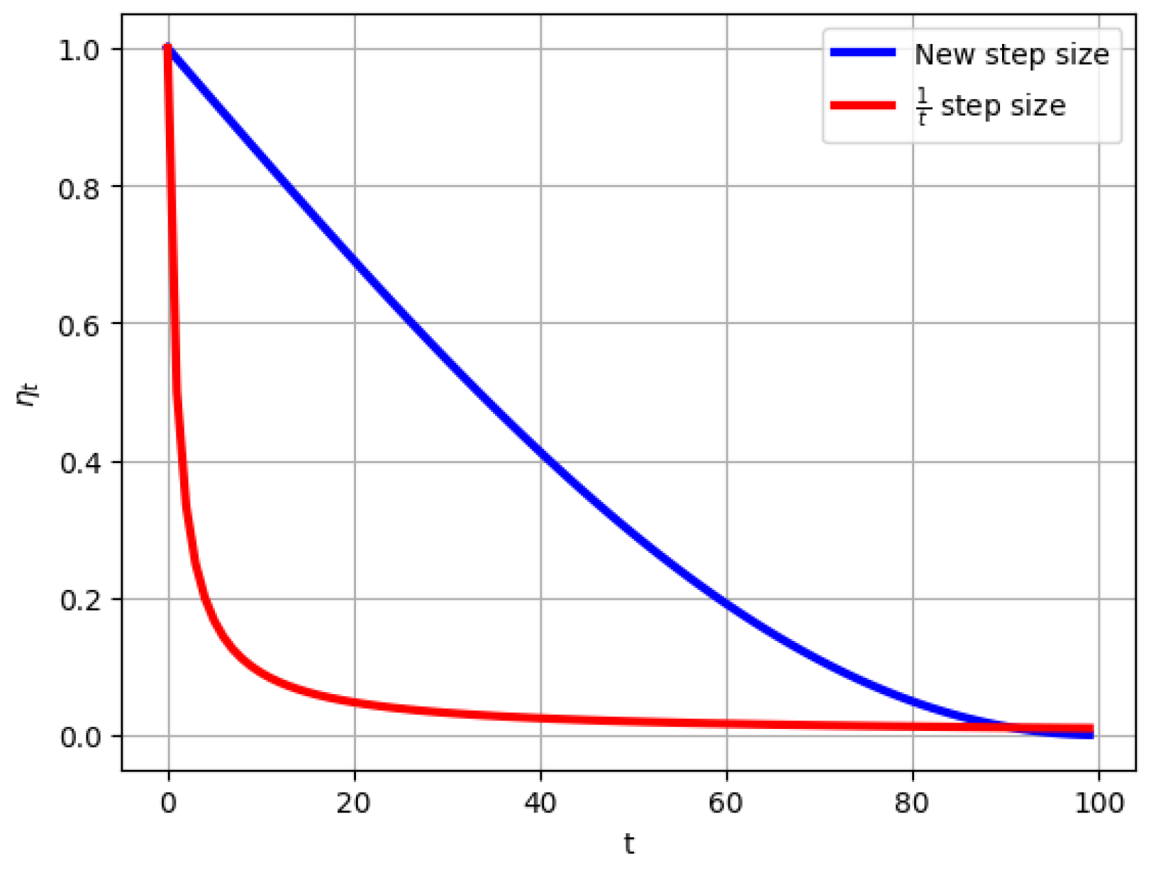
While the step size ${\displaystyle \frac{1}{t}}$ is widely recognized for its theoretical efficiency in SGD, it has a notable drawback; that is, the step size decreases rapidly after only a few iterations. As a result, the updates to the model parameters become progressively smaller, which significantly slows down the convergence process, particularly in the later stages of optimization. This inefficiency has motivated the development of alternative step size strategies to address the limitations of the step size ${\displaystyle \frac{1}{t}}$.

To overcome this issue, we propose a trigonometric step size that ensures a more gradual and smooth decay compared to the steep reduction in the step size ${\displaystyle \frac{1}{t}}$. The new step size is defined as

$${\eta }_t=2{\eta }_0{sin}^2\left({\displaystyle \frac{T-t}{4T}}\pi \right),$$

(3)

where ${\eta }_0$ is the initial step size, and T represents the total number of iterations. This formulation maintains a relatively larger step size during the initial iterations, enabling efficient exploration of the optimization landscape. As training progresses, the step size gradually decreases, allowing for more precise parameter adjustments near the optimal solution. The new trigonometric step size given by (3) provides two key advantages over the step size ${\displaystyle \frac{1}{t}}$:

• Unlike the rapid reduction in the step size ${\displaystyle \frac{1}{t}}$, the proposed step size decreases smoothly over iterations, improving the balance between exploration and exploitation.
• The smoother decay prevents updates from becoming too small in the later stages, ensuring steady and reliable progress toward convergence.

Figure 1 demonstrates the behavior of the new trigonometric step size compared to the step size ${\displaystyle \frac{1}{t}}$, highlighting its smoother and more controlled transition over iterations. This property makes it a promising alternative for improving the efficiency and stability of SGD in various optimization tasks.

2.2. Warm-Restart Stochastic Gradient Descent (SGD)

Warm-restart SGD is an extension of the traditional SGD algorithm that periodically resets the learning rate during optimization. By introducing periodic “restarts” in the learning rate schedule, the method allows the algorithm to escape suboptimal local minima and explore new regions of the solution space, making it particularly effective for non-convex optimization problems [7]. The approach involves starting each cycle with a high learning rate to promote exploration, followed by a gradual reduction to focus on exploitation and fine-tuning. This periodicity and adaptability enable the algorithm to balance exploration and exploitation dynamically, improving its performance across diverse optimization tasks.

The new trigonometric step size, defined by (3), is inherently periodic, making it especially suitable for warm-restart SGD. Its smooth and gradual decay aligns naturally with the cyclical learning rate schedule of warm restarts. At the start of each cycle, the higher values of the step size encourage substantial updates, facilitating effective exploration of new solution regions. As the cycle progresses, the step size decreases smoothly, ensuring consistent and meaningful updates that drive steady convergence. Unlike abrupt decay schedules, the sine-based step size avoids excessively small updates late in the optimization process, maintaining efficiency and stability. By integrating the periodic nature of the trigonometric step size with the warm-restart framework, this approach enhances the algorithm’s adaptability and accelerates convergence, particularly in complex, non-convex optimization landscapes.

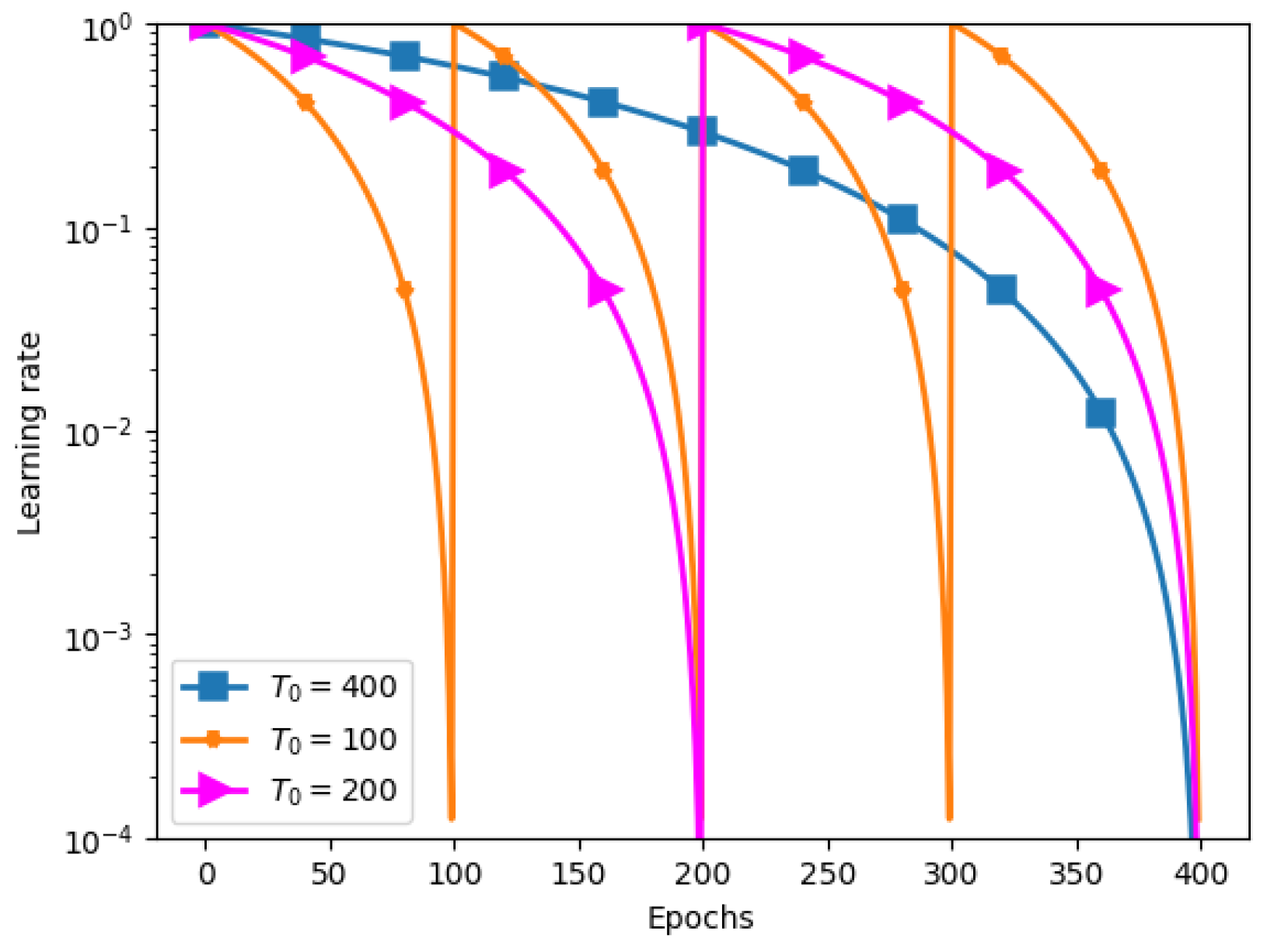
Figure 2 illustrates the performance of the warm-restart strategy combined with the proposed trigonometric step size for various values of the total number of iterations, T, set to 100, 200, and 400. As shown, the step size undergoes a smoother decay compared to traditional strategies, where the gradual reduction in the learning rate allows for larger updates during the earlier stages of training. With different values of T, the figure highlights how the new step size maintains sufficient exploration in the initial phase and provides controlled exploitation in the latter stages, contributing to faster convergence and more efficient optimization. The effect of varying T demonstrates how the decay rate adapts, offering more flexibility in fine-tuning the learning process for different training durations.

2.3. Algorithm

In our proposed approach, as outlined in Algorithm 1, we maintain a uniform number of inner iterations for each outer cycle, ensuring consistency in the algorithm’s performance across all stages. Specifically, the condition $T_0=T_1=\dots =T_l$ indicates that the number of iterations within each epoch is kept constant, simplifying the analysis and comparison of different outer cycles. The algorithm begins by setting the initial parameters, including the initial value for the step size ${\eta }_0$, the initial point $x_0^1$, the total number of inner iterations T, and the number of outer cycles l. In addition, the algorithm is structured into two nested loops. The outer loop iterates through the specified number of epochs l, while the inner loop executes the SGD updates within each epoch, using the proposed sine step size. The step size used for each inner iteration, i.e., t, is defined by

$${\eta }_t=2{\eta }_0{sin}^2\left({\displaystyle \frac{T-t}{4T}}\pi \right).$$

At the end of each inner loop, the updated point $x_i^T$ is passed to the next outer iteration as the starting point $x_{i+1}^1$, ensuring continuity between epochs. Once all outer iterations are complete, the algorithm returns the final optimized point $x^{*}=x_l^T$.

3. Convergence

This section is dedicated to a theoretical analysis establishing the convergence properties of the SGD algorithm under the proposed step size. The analysis addresses smooth non-convex objective functions, with particular attention given to scenarios both satisfying and not satisfying the Polyak–Łojasiewicz (PL) condition. To facilitate this analysis, we introduce several key lemmas that play a critical role in establishing the convergence properties of the SGD algorithm with the new sine step size.

3.1. Convergence Without the PL Condition

We demonstrate that the SGD algorithm, utilizing the proposed step size for smooth non-convex functions, attains a convergence rate of $O\left({\displaystyle \frac{1}{\sqrt{T}}}\right)$, matching the best-known theoretical rate. The next lemma provides both an upper and lower bound for the function $sin\left(x\right)$, when $x\in \left[0,{\displaystyle \frac{\pi }{2}}\right]$.

Lemma 1. 

For all $x\in [0,{\displaystyle \frac{\pi }{2}}]$, we have:

• $sinx\ge {\displaystyle \frac{2}{\pi }}x$;
• $sinx\le x$.

Lemma 2. 

For the step size given by (3), we have 

$$\sum _{t=1}^T{\eta }_t\ge {\displaystyle \frac{{\eta }_0(T-1)}{6}}.$$

Proof. 

Using Lemma 1, we have

$$\begin{array}{ccc}\hfill \sum _{t=1}^T{\eta }_t& =& 2{\eta }_0\sum _{t=1}^T{sin}^2\left({\displaystyle \frac{T-t}{4T}}\pi \right)\ge {\displaystyle \frac{8{\eta }_0}{{\pi }^2}}\sum _{t=1}^T{\left({\displaystyle \frac{T-t}{4T}}\pi \right)}^2\hfill \\ & =& {\displaystyle \frac{{\eta }_0}{2T^2}}\sum _{t=1}^T{t}^2={\displaystyle \frac{{\eta }_0}{2T^2}}{\int }_1^T{t}^{2}dt\ge {\displaystyle \frac{{\eta }_0(T-1)}{6}}.\hfill \end{array}$$

 □

The next lemma provides an upper bound for ${\sum }_{t=1}^T{\eta }_t^2$.

Lemma 3. 

For the step size given by (3), we have 

$$\sum _{t=1}^T{\eta }_t^2\le {\displaystyle \frac{{\pi }^4{\eta }_0^{2}T}{20}}.$$

Proof. 

Using Lemma 1, we have

$$\begin{array}{ccc}\hfill \sum _{t=1}^T{\eta }_t^2& =& 4{\eta }_0^2\sum _{t=1}^T{sin}^4\left({\displaystyle \frac{T-t}{4T}}\pi \right)\le 4{\pi }^4{\eta }_0^2\sum _{t=1}^T{\left({\displaystyle \frac{T-t}{2T}}\right)}^4\hfill \\ & =& {\displaystyle \frac{{\pi }^4{\eta }_0^2}{4T^4}}{\int }_1^T{t}^{4}dt\le {\displaystyle \frac{{\pi }^4{\eta }_0^{2}T}{20}}.\hfill \end{array}$$

 □

The next lemma provides an upper bound for the expected gradient, which depends on the change in the objective function and the step size in SGD, under the condition that f is L-smooth and ${\eta }_t\le {\displaystyle \frac{1}{L}}$.

Lemma 4 

(Lemma 7.1 in [8]). Assuming that f is an L-smooth function and that Assumption A3 holds, if ${\eta }_t\le {\displaystyle \frac{1}{L}}$, then the SGD algorithm guarantees the following results:

$${\displaystyle \frac{{\eta }_t}{2}}\mathbb{E}[\parallel \nabla f\left(x_t\right){\parallel }^2]\le \mathbb{E}\left[f\left(x_t\right)\right]-\mathbb{E}\left[f\left(x_{t+1}\right)\right]+{\displaystyle \frac{L{\eta }_t^2{\sigma }^2}{2}}.$$

(4)

The next theorem establishes an $O\left({\displaystyle \frac{1}{\sqrt{T}}}\right)$ convergence rate of the SGD based on the new step size for smooth non-convex functions without the PL condition.

Theorem 1. 

Under Assumptions A1 and A3, the SGD algorithm with the new step sizes guarantees that 

$$\mathbb{E}|\nabla f\left({\overline{x}}_T\right){|}^2\le {\displaystyle \frac{12}{L\sqrt{T}}}\left(f\left(x_1\right)-f^{*}\right)+{\displaystyle \frac{3{\pi }^4{\sigma }^2}{10\sqrt{T}}},$$

 where ${\overline{x}}_T$ is a random iterate drawn from the sequence $x_1,\dots ,x_T$, with corresponding probabilities $p_1,\dots ,p_T$. The probabilities $p_t$ are defined as $p_t={\displaystyle \frac{{\eta }_t}{{\sum }_{i=1}^T{\eta }_i}}$.

Proof. 

Using the fact that ${\overline{x}}_T$ is randomly selected from the sequence ${\left\{x_t\right\}}_{t=1}^T$ with a probability $P_t={\displaystyle \frac{{\eta }_t}{{\sum }_{t=1}^T{\eta }_t}}$ and applying Jensen’s inequality, we obtain

$$\begin{array}{ccc}& & \mathbb{E}[\parallel \nabla f\left({\overline{x}}_T\right){\parallel }^2]\le {\displaystyle \frac{{\sum }_{t=1}^T{\eta }_t\mathbb{E}[\parallel \nabla f\left(x_t\right){\parallel }^2]}{{\sum }_{t=1}^T{\eta }_t}}\hfill \\ & \le & {\displaystyle \frac{2{\sum }_{t=1}^T\left[\mathbb{E}\left[f\left(x_t\right)\right]-\mathbb{E}\left[f\left(x_{t+1}\right)\right]\right]}{{\sum }_{t=1}^T{\eta }_t}}+{\displaystyle \frac{L{\sigma }^2{\sum }_{t=1}^T{\eta }_t^2}{{\sum }_{t=1}^T{\eta }_t}}.\hfill \end{array}$$

We obtain the first and second inequalities by applying Jensen’s inequality and utilizing Lemma 4. Furthermore, considering the fact that $f\left(x_{T+1}\right)\ge f^{*}$ and Lemmas 2 and 3, we obtain

$$\begin{array}{ccc}\hfill \mathbb{E}[\parallel \nabla f\left({\overline{x}}_T\right){\parallel }^2]& \le & {\displaystyle \frac{2\left(f\left(x_1\right)-f^{*}\right)}{{\sum }_{t=1}^T{\eta }_t}}+{\displaystyle \frac{L{\sigma }^2{\sum }_{t=1}^T{\eta }_t^2}{{\sum }_{t=1}^T{\eta }_t}}\hfill \\ & \le & {\displaystyle \frac{12\left(f\left(x_1\right)-f^{*}\right)}{{\eta }_0(T-1)}}+{\displaystyle \frac{L{\sigma }^2{\eta }_0^2\frac{3T{\pi }^4}{10}}{{\eta }_0(T-1)}}\hfill \\ & =& {\displaystyle \frac{12Lc}{T-1}}\left(f\left(x_1\right)-f^{*}\right)+{\displaystyle \frac{3L{\sigma }^2{\pi }^{4}T}{10Lc(T-1)}}.\hfill \end{array}$$

Setting $c=O\left(\sqrt{T}\right)$, we can conclude that

$$\begin{array}{c}\hfill \mathbb{E}[\parallel \nabla f\left({\overline{x}}_T\right){\parallel }^2]\le {\displaystyle \frac{12}{L\sqrt{T}}}\left(f\left(x_1\right)-f^{*}\right)+{\displaystyle \frac{3{\pi }^4{\sigma }^2}{10\sqrt{T}}}.\end{array}$$

□

3.2. Convergence Results with PL Condition

The PL condition is a weaker form of strong convexity often used in the analysis of optimization algorithms. This property allows SGD to achieve efficient convergence, even for non-convex loss functions. Here, we present the convergence results for SGD with the new step size under the PL condition for smooth non-convex functions. Our analysis shows that the proposed sine step size achieves a convergence rate of $O\left({\displaystyle \frac{1}{{\mu }^{5/3}{T}^{2/3}}}\right)$. We begin by presenting several lemmas that are crucial for proving this convergence rate.

Lemma 5 

(Lemma 2 in [20]). Suppose $X_k$, $A_k$, $B_k$ are non-negative for all $k\ge 1$, and $X_{k+1}\le A_k{X}_k+B_k$. Then, we have

$$\begin{array}{c}\hfill X_{k+1}\le \prod _{i=1}^k{A}_i{X}_1+\sum _{i=1}^k\prod _{j=i+1}^k{A}_j{B}_i.\end{array}$$

The next lemma establishes an upper bound on the difference between the expected objective function value after T iterations and the optimal value $f^{*}$ for SGD, where the step size ${\eta }_t\le {\displaystyle \frac{1}{L}}$, and f is an L-smooth function that satisfies the PL condition.

Lemma 6. 

Assuming that f is an L-smooth function that satisfies the PL condition and that the step size satisfies ${\eta }_t\le {\displaystyle \frac{1}{L}}$ for all t, the following result holds:

$$\begin{array}{ccc}\hfill \mathbb{E}\left[f\left(x_{T+1}\right)\right]-f^{*}& \le & exp(-\mu \sum _{t=1}^T{\eta }_t)(f\left(x_1\right)-f^{*})+{\displaystyle \frac{L{\sigma }^2}{2}}\sum _{t=1}^{T}exp(-\mu \sum _{i=t+1}^T{\eta }_i){\eta }_t^2.\hfill \end{array}$$

Proof. 

From Lemma 4 we have

$$\begin{array}{c}\hfill \mathbb{E}\left[f\left(x_{t+1}\right)\right]\le \mathbb{E}\left[f\left(x_t\right)\right]-{\displaystyle \frac{{\eta }_t}{2}}\mathbb{E}[\parallel \nabla f\left(x_t\right){\parallel }^2]+{\displaystyle \frac{L{\eta }_t^2{\sigma }^2}{2}}.\end{array}$$

(5)

Equation (5) can be written as

$$\begin{array}{c}\hfill \mathbb{E}\left[f\left(x_{t+1}\right)\right]-f^{*}\le \mathbb{E}\left[f\left(x_t\right)\right]-f^{*}-{\displaystyle \frac{{\eta }_t}{2}}\mathbb{E}[\parallel \nabla f\left(x_t\right){\parallel }^2]+{\displaystyle \frac{L{\eta }_t^2{\sigma }^2}{2}}.\end{array}$$

By utilizing the PL condition, i.e., ${\displaystyle \frac{1}{2}}\mathbb{E}\left[\right|\nabla f\left(x_t\right){|}^2]\ge \mu (\mathbb{E}\left[f\left(x_t\right)\right]-f^{*})$, we conclude that

$$\begin{array}{c}\hfill \mathbb{E}\left[f\left(x_{t+1}\right)\right]-f^{*}\le (1-\mu {\eta }_t)(\mathbb{E}\left[f\left(x_t\right)\right]-f^{*})+{\displaystyle \frac{L{\eta }_t^2{\sigma }^2}{2}}.\end{array}$$

(6)

We now define ${\Delta }_t=\mathbb{E}\left[f\left(x_t\right)\right]-f^{*}$. As a result, from (6) we derive

$$\begin{array}{c}\hfill {\Delta }_{t+1}\le (1-\mu {\eta }_t){\Delta }_t+{\displaystyle \frac{L}{2}}{\eta }_t^2{\sigma }^2.\end{array}$$

Utilizing Lemma 5 along with the definition of ${\Delta }_t$, the following inequality can be established:

$$\begin{array}{c}\hfill {\Delta }_{T+1}\le \prod _{t=1}^T(1-\mu {\eta }_t){\Delta }_1+{\displaystyle \frac{L}{2}}\sum _{t=1}^T\prod _{i=t+1}^T(1-\mu {\eta }_i){\eta }_t^2{\sigma }^2.\end{array}$$

(7)

Using the fact that $1-x\le exp(-x)$ and leveraging the property ${\prod }_{i=1}^{k}exp\left(x_i\right)=exp\left({\sum }_{i=1}^k{x}_i\right)$, Equation (7) can be reformulated as

$$\begin{array}{c}\hfill {\Delta }_{T+1}\le exp(-\mu \sum _{t=1}^T{\eta }_t){\Delta }_1+{\displaystyle \frac{L{\sigma }^2}{2}}\sum _{t=1}^{T}exp(-\mu \sum _{i=t+1}^T{\eta }_i){\eta }_t^2.\end{array}$$

 □

Lemma 7. 

Let $a,b$ be non-negative numbers. Then, we have 

$$\begin{array}{c}\hfill \sum _{t=0}^{T}exp(-bt)t^a\le 2exp(-a){\left({\displaystyle \frac{a}{b}}\right)}^a+{\displaystyle \frac{\Gamma (a+1)}{b^{a+1}}}.\end{array}$$

Proof. 

We define the function $f\left(t\right)=exp(-bt)t^a$, where $a,b\ge 0$. It is clear that the function $f\left(t\right)$ is increasing on the interval $\left[0,{\displaystyle \frac{a}{b}}\right]$ and decreasing for $t\ge {\displaystyle \frac{a}{b}}$. Therefore, the summation

$$S=\sum _{t=0}^{T}exp(-bt)t^a$$

can be bounded by partitioning the sum around $t=a/b$. Specifically, we decompose S as follows:

$$S=\sum _{t=0}^{⌊a/b⌋-1}exp(-bt)t^a+exp(-a){\left({\displaystyle \frac{a}{b}}\right)}^a+exp(-a){\left({\displaystyle \frac{a}{b}}\right)}^a+\sum _{t=⌊a/b⌋+1}^{T}exp(-bt)t^a.$$

An upper bound for ${\sum }_{t=0}^{⌊a/b⌋-1}exp(-bt)t^a$ can be written as

$$\sum _{t=0}^{⌊a/b⌋-1}exp(-bt)t^a\le {\int }_0^{a/b}exp(-bt)t^{a}dt.$$

Moreover, we have

$$\sum _{t=⌊a/b⌋+1}^{T}exp(-bt)t^a\le {\int }_{a/b}^{T}exp(-bt)t^{a}dt\le {\int }_{a/b}^{\infty }exp(-bt)t^{a}dt.$$

Therefore, we can conclude that

$$S\le 2exp(-a){\left({\displaystyle \frac{a}{b}}\right)}^a+{\int }_0^{\infty }exp(-bt)t^{a}dt.$$

Using the fact that ${\int }_0^{\infty }exp(-bt)t^{a}dt={\displaystyle \frac{\Gamma (a+1)}{b^{a+1}}}$, we obtain

$$S\le 2exp(-a){\left({\displaystyle \frac{a}{b}}\right)}^a+{\displaystyle \frac{\Gamma (a+1)}{b^{a+1}}}.$$

 □

In order to use Lemma 6, it is essential to derive a lower bound for ${\sum }_{i=t+1}^T{\eta }_i$ and an upper bound for ${\sum }_{t=1}^{T}exp\left(-\mu {\sum }_{i=t+1}^T{\eta }_i\right){\eta }_t^2$. The subsequent lemma establishes these bounds.

Lemma 8. 

For the new proposed step size, as defined in (3), the following bounds hold:

I. 

${\sum }_{i=t+1}^T{\eta }_i\ge {\eta }_0{\displaystyle \frac{{(T-t-t)}^3}{6T^2}}$.

II. 

${\sum }_{t=1}^{T}exp\left(-\mu {\sum }_{i=t+1}^T{\eta }_i\right){\eta }_t^2\le 4{\eta }_0{\left({\displaystyle \frac{\pi }{4T}}\right)}^4\left(2exp(-{\displaystyle \frac{4}{3}}){\left({\displaystyle \frac{8T^2}{\mu }}\right)}^{{\displaystyle \frac{4}{3}}}+\Gamma \left({\displaystyle \frac{5}{3}}\right){\left({\displaystyle \frac{6T^2}{\mu }}\right)}^{{\displaystyle \frac{5}{3}}}\right)$

Proof. 

To prove item (I), we apply the definition of ${\eta }_t$ and use Lemma 1. Therefore, we have

$$\begin{array}{ccc}\hfill \sum _{i=t+1}^T{\eta }_i& \ge & 2{\eta }_0{\left({\displaystyle \frac{2}{\pi }}\right)}^2\sum _{i=t+1}^T{\left({\displaystyle \frac{T-i}{4T}}\pi \right)}^2={\displaystyle \frac{{\eta }_0}{2T^2}}\sum _{i=0}^{T-t-1}{i}^2\hfill \\ & =& {\displaystyle \frac{{\eta }_0}{2T^2}}{\int }_0^{T-t-1}{i}^{2}di={\eta }_0{\displaystyle \frac{{(T-t-t)}^3}{6T^2}}.\hfill \end{array}$$

(8)

To prove item (II), we use Equation (8), which leads to the following conclusion:

$$\begin{array}{ccc}\hfill \sum _{t=1}^{T}exp\left(-\mu \sum _{i=t+1}^T{\eta }_i\right){\eta }_t^2& \le & 4{\eta }_0^2\sum _{t=1}^{T}exp\left(-\mu {\displaystyle \frac{{\eta }_0{(T-t-1)}^3}{6T^2}}\right){sin}^4\left({\displaystyle \frac{T-t}{4T}}\pi \right)\hfill \\ & \le & 4{\eta }_0^2{\left({\displaystyle \frac{\pi }{4T}}\right)}^4\sum _{t=1}^T{(T-t)}^{4}exp\left(-{\displaystyle \frac{\mu {\eta }_0{(t-1)}^3}{6T^2}}\right)\hfill \\ & \le & 4{\eta }_0^2{\left({\displaystyle \frac{\pi }{4T}}\right)}^4\sum _{t=0}^{T-1}{t}^{4}exp\left(-{\displaystyle \frac{\mu {\eta }_0{(t-1)}^3}{6T^2}}\right)\hfill \\ & \le & 4{\eta }_0^2{\left({\displaystyle \frac{\pi }{4T}}\right)}^4\sum _{t=1}^{T-1}{t}^{4}exp\left(-{\displaystyle \frac{\mu {\eta }_0{t}^3}{6T^2}}\right)\hfill \\ & \le & 4{\eta }_0{\left({\displaystyle \frac{\pi }{4T}}\right)}^4\left(2exp(-{\displaystyle \frac{4}{3}}){\left({\displaystyle \frac{8T^2}{\mu }}\right)}^{{\displaystyle \frac{4}{3}}}+\Gamma \left({\displaystyle \frac{5}{3}}\right){\left({\displaystyle \frac{6T^2}{\mu }}\right)}^{{\displaystyle \frac{5}{3}}}\right),\hfill \end{array}$$

(9)

where the last inequality is obtained by using Lemma 7. □

By combining the results from Lemmas 2, 6 and 8, we can establish the convergence rate for smooth non-convex functions under the PL condition.

Theorem 2. 

Consider the SGD algorithm with the new proposed step size. Under Assumptions A1–A3, and for a given number of iterations T with the initial step size ${\eta }_0={\displaystyle \frac{1}{L}}$, the algorithm delivers the following guarantees: 

$$\begin{array}{ccc}\hfill \mathbb{E}\left[f\left(x_{T+1}\right)\right]-f^{*}& \le & exp(-\mu {\displaystyle \frac{T-1}{6L}})\left[\mathbb{E}\left[f\left(x_1\right)\right]-f^{*}\right]\hfill \\ & +& {\displaystyle \frac{\pi }{196L{T}^4}}\left(2exp(-{\displaystyle \frac{4}{3}}){\left({\displaystyle \frac{8T^2}{\mu }}\right)}^{{\displaystyle \frac{4}{3}}}+\Gamma \left({\displaystyle \frac{5}{3}}\right){\left({\displaystyle \frac{6T^2}{\mu }}\right)}^{{\displaystyle \frac{5}{3}}}\right).\hfill \end{array}$$

Proof. 

From Lemma 6, we have

$$\begin{array}{ccc}\hfill \mathbb{E}\left[f\left(x_{T+1}\right)\right]-f^{*}& \le & exp(-\mu \sum _{t=1}^T{\eta }_t)(\mathbb{E}\left[f\left(x_1\right)\right]-f^{*}){\displaystyle \frac{L{\sigma }^2}{2}}\sum _{t=1}^{T}exp(-\mu \sum _{i=t+1}^T{\eta }_i){\eta }_t^2.\hfill \end{array}$$

(10)

Using Lemmas 2 and 8, we can rewrite (10) as

$$\begin{array}{ccc}\hfill \mathbb{E}\left[f\left(x_{T+1}\right)\right]-f^{*}& \le & exp(-\mu {\eta }_0{\displaystyle \frac{T-1}{6}})\left[\mathbb{E}\left[f\left(x_1\right)\right]-f^{*}\right]\hfill \\ & +& 4{\eta }_0^2{\left({\displaystyle \frac{\pi }{4T}}\right)}^4\left(2exp(-{\displaystyle \frac{4}{3}}){\left({\displaystyle \frac{8T^2}{\mu }}\right)}^{{\displaystyle \frac{4}{3}}}+\Gamma \left({\displaystyle \frac{5}{3}}\right){\left({\displaystyle \frac{6T^2}{\mu }}\right)}^{{\displaystyle \frac{5}{3}}}\right).\hfill \end{array}$$

Setting ${\eta }_0={\displaystyle \frac{1}{L}}$, we conclude that

$$\begin{array}{ccc}\hfill \mathbb{E}\left[f\left(x_{T+1}\right)\right]-f^{*}& \le & exp(-\mu {\displaystyle \frac{T-1}{6L}})\left[\mathbb{E}\left[f\left(x_1\right)\right]-f^{*}\right]\hfill \\ & +& {\displaystyle \frac{\pi }{196L{T}^4}}\left(2exp(-{\displaystyle \frac{4}{3}}){\left({\displaystyle \frac{8T^2}{\mu }}\right)}^{{\displaystyle \frac{4}{3}}}+\Gamma \left({\displaystyle \frac{5}{3}}\right){\left({\displaystyle \frac{6T^2}{\mu }}\right)}^{{\displaystyle \frac{5}{3}}}\right).\hfill \end{array}$$

 □

Based on Theorem 2, we can conclude that the SGD algorithm with the newly proposed step size, for a smooth non-convex function satisfying the PL condition, achieves a convergence rate of $O\left({\displaystyle \frac{1}{{\mu }^{5/3}{T}^{2/3}}}\right)$.

4. Numerical Results

In this section, we assess the performance of the proposed algorithm on image classification tasks by comparing its effectiveness against state-of-the-art methods across three widely used datasets: FashionMNIST, CIFAR10, and CIFAR100 [2].

The FashionMNIST dataset consists of 50,000 grayscale images for training and 10,000 examples for testing, each with dimensions of $28\times 28$ pixels. For this dataset, we utilize a convolutional neural network (CNN) model. The architecture comprises two convolutional layers with kernel sizes of $5\times 5$ and padding of 2, followed by two max-pooling layers with kernel sizes of $2\times 2$. The model also includes two fully connected layers, each with 1024 hidden nodes, employing the rectified linear unit (ReLU) activation function. To prevent overfitting, dropout with a rate of $0.5$ is applied to the hidden layers of the network. For performance evaluation, we use the cross-entropy loss function and measure accuracy as the primary evaluation metric for comparing the performance of the different algorithms.

The CIFAR10 dataset comprises 60,000 color images of size $32\times 32$, which are divided into 10 classes with 6000 images each. The dataset is split into 50,000 training images and 10,000 test images. To evaluate algorithm performance on this dataset, a 20-layer residual neural network (ResNet) architecture, as introduced in [25], is employed. The ResNet model employs cross-entropy as the loss function.

The CIFAR100 dataset shares similarities with CIFAR10, with the key difference being that it consists of 100 classes, each containing 600 distinct natural images. For each class, there are 500 training images and 100 testing images. To enhance the training process, randomly cropped and flipped images are utilized. The deep learning model employed is a DenseNet-BC model that consists of 100 layers, with a growth rate of 12 [26].

We conducted a performance comparison between our proposed method and state-of-the-art methods that have been previously fine-tuned in a study in [20]. In our own numerical studies, we adopted the same hyperparameter values as used in that research. To mitigate the impact of stochasticity, the experiments are repeated five times using random seeds.

4.1. Methods

In our study, we examined SGD with various step sizes as follows:

• ${\eta }_t=constant$;
• ${\eta }_t={\displaystyle \frac{{\eta }_0}{1+\alpha \sqrt{t}}}$;
• ${\eta }_t={\displaystyle \frac{{\eta }_0}{1+\alpha t}}$;
• ${\eta }_t={\displaystyle \frac{{\eta }_0}{2}}\left(1+cos{\displaystyle \frac{t\pi }{T}}\right)$;
• ${\eta }_t={\eta }_0(1-cos\left({\displaystyle \frac{T-t}{2T}}\pi \right))$.

We give the following names to these step sizes: the SGD constant step size, the $O\left({\displaystyle \frac{1}{\sqrt{t}}}\right)$ step size, the $O\left({\displaystyle \frac{1}{t}}\right)$ step size, and the new step size. The parameter t represents the iteration number of the inner loop, and each outer iteration consists of iterations for training on mini-batches. We wanted to compare the performance of the new step size with other optimization methods, namely, Adam, SGD + Armijo, PyTorch’s ReduceLROnPlateau scheduler, and the stagewise step size method. It is worth noting that the term “stagewise” in our context refers to the Stagewise—2 Milestone and Stagewise—3 Milestone methods, as defined in [20]. Since we utilized Nesterov momentum in all our SGD variants, the performance of multistage accelerated algorithms, as discussed in [27], is essentially covered by the stagewise step decay. For consistency, all our experiments followed the settings proposed in [20].

4.2. Parameters

To determine the optimal value for the hyperparameter ${\eta }_0$ for each dataset, we employed a two-stage grid search approach. In the first stage, we conducted a coarse search using the grid $\{0.00001,0.0001,0.001,0.01,0.1,0.2,0.3,0.4,0.5,0.6,0.7,0.8,0.9,1\}$ to identify a promising interval for ${\eta }_0$ that yielded the best validation performance. In the second stage, we further refined the search within the identified interval by dividing it into 10 equally spaced values and evaluating the accuracy at each point. This fine-tuning process allowed us to determine the optimal ${\eta }_0$ for each dataset based on the resulting performance. The procedure was applied individually to each dataset, ensuring that the hyperparameters were specifically tailored to the characteristics of each dataset.

To benchmark the effectiveness of our proposed method, we compared it against state-of-the-art approaches. The hyperparameters used for these methods were obtained from a prior study [20], and we adopted the same values in our experiments for consistency. These hyperparameters are summarized in

Table 1. The hyperparameter values for the methods employed on the FashionMNIST, CIFAR10, and CIFAR100 datasets.

	FashionMNIST			CIFAR10			CIFAR100
Methods	${\mathit{\eta }}_{\mathbf{0}}$	$\mathit{\alpha }$	$\mathit{c}$	${\mathit{\eta }}_{\mathbf{0}}$	$\mathit{\alpha }$	$\mathit{c}$	${\mathit{\eta }}_{\mathbf{0}}$	$\mathit{\alpha }$	$\mathit{c}$
Constant step size	$0.007$	−	−	$0.07$	−	−	$0.07$	−	−
$O\left({\displaystyle \frac{1}{t}}\right)$ step size	$0.05$	$0.00038$	−	$0.1$	$0.00023$	−	$0.8$	$0.004$	−
$O\left({\displaystyle \frac{1}{\sqrt{t}}}\right)$ step size	$0.05$	$0.00653$	−	$0.2$	$0.07907$	−	$0.1$	$0.015$	−
Adam	$0.0009$	−	−	$0.0009$	−	−	$0.0009$	−	−
SGD + Armijo	$0.5$	−	$0.1$	$2.5$	−	$0.1$	5	−	$0.5$
ReduceLROnPlateau	$0.04$	$0.5$	−	$0.07$	$0.1$	−	$0.1$	$0.5$	−
Stagewise—1 Milestone	$0.04$	$0.1$	−	$0.1$	$0.1$	−	$0.07$	$0.1$	−
Stagewise—2 Milestone	$0.04$	$0.1$	−	$0.2$	$0.1$	−	$0.07$	$0.1$	−
New step size	$0.02$	−	−	$0.25$	−	−	$0.13$	−	−

. The momentum parameter was fixed at 0.9 across all methods and datasets. Moreover, the symbol − indicates that the respective step size does not require or utilize the specified parameter. For weight decay, we used values of $0.0001$ for FashionMNIST and CIFAR10, and $0.0005$ for CIFAR100, consistent across all methods. Additionally, a batch size of 128 was used for all experiments. The parameter $T_0$ was defined as the ratio of the number of training samples to the batch size.

4.3. Results and Discussion

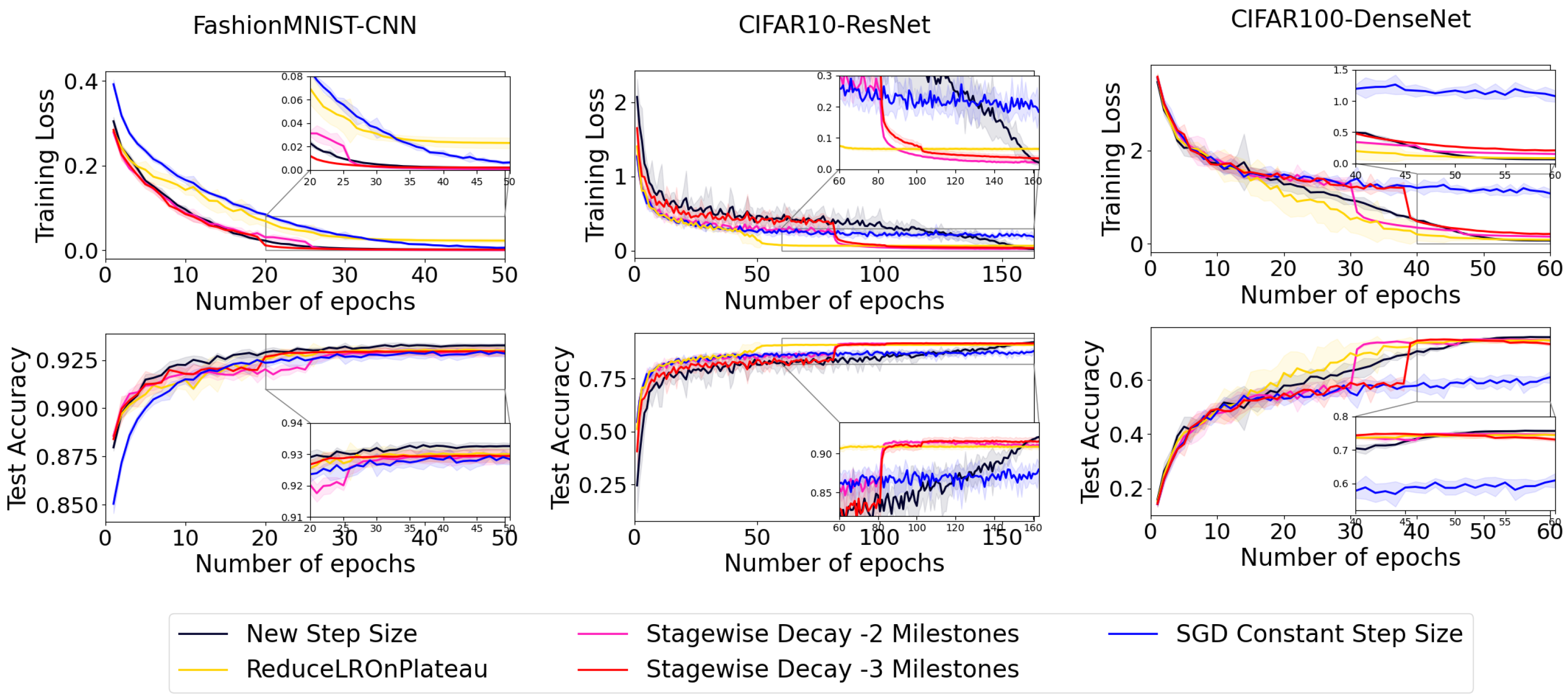
We divide the methods into two groups and present the results in distinct figures for better clarity. In Figure 3 and Figure 4, we observe that the new proposed step size shows significant improvements on the FashionMNIST dataset. After the 40th epoch, it achieves a training loss close to zero, comparable to the well-known methods SGD + Armijo and Stagewise—3 Milestone. Additionally, the test accuracy of the new proposed step size surpasses all other methods in this dataset.

In the CIFAR10 dataset, the new step size achieves superior accuracy compared to other step sizes. Specifically, it enhances the accuracy of Stagewise—2 Milestone by $0.91\%$ in test accuracy, as shown in Figure 3 and Figure 4. Similarly, in the CIFAR100 dataset, this new step size outperforms others in terms of accuracy, improving the accuracy of Stagewise—1 Milestone by $1.14\%$ in test accuracy, as evidenced in Figure 3 and Figure 4.

Overall, the newly proposed step size demonstrates the best performance among the methods evaluated for both the CIFAR10 and CIFAR100 datasets, as clearly indicated in Figure 3 and Figure 4.

Table 2. Average final test accuracy obtained by 5 runs starting from different random seeds; ± is followed by an estimated margin of error under $95\%$ confidence.

Step Size	FashionMNIST	CIFAR10	CIFAR100
Constant Step Size	$0.9299\pm 0.0016$	$0.8776\pm 0.0060$	$0.6089\pm 0.01485$
$O\left({\displaystyle \frac{1}{t}}\right)$ Step Size	$0.9311\pm 0.0012$	$0.8946\pm 0.0020$	$0.6885\pm 0.0051$
$O\left({\displaystyle \frac{1}{\sqrt{t}}}\right)$ Step Size	$0.9275\pm 0.0007$	$0.8747\pm 0.0077$	$0.6411\pm 0.00469$
Adam	$0.9166\pm 0.0019$	$0.8839\pm 0.0031$	$0.6555\pm 0.00430$
SGD + Armijo	$0.9277\pm 0.0012$	$0.8834\pm 0.0059$	$0.6869\pm 0.00460$
ReduceLROnPlateau	$0.9299\pm 0.0014$	$0.9081\pm 0.0019$	$0.7440\pm 0.00695$
Stagewise—1 Milestone	$0.9303\pm 0.0007$	$0.9111\pm 0.0034$	$0.7456\pm 0.00188$
Stagewise—2 Milestone	$0.9298\pm 0.0014$	$0.9151\pm 0.0039$	$0.73102\pm 0.00402$
New step size	0.9326 ± 0.0007	0.9206 ± 0.0006	0.7570 ± 0.0012

demonstrates the average of the final test accuracy obtained by five runs starting from different random seeds on the FashionMNIST, CIFAR10, and CIFAR100 datasets. The bolded values in the table represent the highest accuracy achieved for each dataset among all different step sizes. Based on the information presented in Table 2, it can be inferred that the new proposed step size leads to a $0.15\%$, $0.91\%$, and $1.14\%$ improvement in test accuracy compared to the previously studied best method on the FashionMNIST, CIFAR10, and CIFAR100 datasets, respectively.

4.4. Limitations

The proposed step size has demonstrated notable performance improvements when applied to the DenseNet-BC model for classification tasks. However, a significant limitation arises when attempting to extend this approach to more complex neural network architectures, such as EfficientNet. These models, which require the updating of a larger number of weight parameters, introduce substantial computational complexity. Moreover, the current system is constrained by limited GPU and hardware resources, which restricts the ability to efficiently explore hyperparameter configurations for these advanced architectures. This makes it challenging to fully leverage the potential of the proposed step size in more complex models.

5. Conclusions

In this paper, we introduced a novel sine step size aimed at enhancing the efficiency of the stochastic gradient descent (SGD) algorithm, particularly for optimizing smooth non-convex functions. We derived a theoretical convergence rate for SGD based on the newly proposed step size for smooth non-convex functions, both with and without the PL condition. By testing the approach on image classification tasks using the FashionMNIST, CIFAR10, and CIFAR100 datasets, we observed significant improvements in accuracy, with gains of $0.15\%$, $0.91\%$, and $1.14\%$, respectively. These findings highlight the potential of the sine step size in advancing optimization techniques for deep learning, paving the way for further exploration and application in complex machine learning tasks.

For future work, testing the sine step size on more complex neural network architectures like recurrent neural networks (RNNs) and transformers could provide further insights into its effectiveness across a wider range of tasks. Exploring its impact on large-scale datasets and different domains, such as natural language processing or reinforcement learning, could also enhance its applicability. Finally, theoretical advancements in convergence analysis for different types of functions, including convex and strongly convex problems, could refine its usage in diverse optimization scenarios.