Stability of Differential Equations with Random Impulses and Caputo-Type Fractional Derivatives

Abstract

In this paper, we study nonlinear differential equations with Caputo fractional derivatives with respect to other functions and impulses. The main characteristic of the impulses is that the time between two consecutive impulsive moments is defined by random variables. These random variables are independent. As the distribution of these random variables is very important, we consider the Erlang distribution. It generalizes the exponential distribution, which is very appropriate for describing the time between the appearance of two consecutive events. We describe a detailed solution to the studied problem, which is a stochastic process. We define the p-exponential stability of the solutions and obtain sufficient conditions. The study is based on the application of appropriate Lyapunov functions. The obtained sufficient conditions depend not only on the nonlinear function and impulsive functions, but also on the function used in the fractional derivative. The obtained results are illustrated using some examples.

1. Introduction

Many evolution processes are characterized by abrubt changes in state and their adequate models are impulsive differential equations. Several examples of models by stochastic differential equations with random impulses in engineering, such as the vibration of plates and shells, and of nonlinear oscillators under random impulses, are provided in the book [1]. In the case of dynamics of real-world phenomena and processes is modeled by deterministic equations and they have instantaneous changes at random moments, we need to use another model. This model combines the deterministic differential equations and impulses at random moments, i.e., we have to use so called impulsive differential equations with random impulses. The study of these equations requires a combination of the qualitative theory of differential equations and probability theory. Impulsive differential equations with random impulsive moments differ from the study of stochastic differential equations with jumps (see, for example, [2,3,4,5,6]).

In this paper, we study nonlinear fractional differential equations with random impulses. It is well known that the waiting time between two consecutive events is best described by an exponential distribution. To be more general, we consider Erlang distribution, which is a generalization of exponential distribution. The time between two consecutive impulses is described by independent Erlang distributed random variables. Similar problems, focusing on the case where random moments follow an exponential distribution, are studied in [7], while ordinary differential equations with Erlang-distributed random variables are considered in [8]. To be more general, we apply a Caputo fractional derivative with respect to another function. The application of this type of derivative is not only a generalization of the published results, but it has a huge influence on the sufficient conditions (see Remark 4) and provides opportunities to model some phenomena more adequately. Any solution to the studied problem is a stochastic process and it has been well defined in the paper. At the same time, the solutions of stochastic differential equations are also stochastic processes, but the situation is totally different than in the studied case (see, for example, [9]). The p-moment exponential stability of the trivial solution is defined similarly to the case of stochastic equations and studied by employing Lyapunov functions.

2. Notes on Fractional Calculus

Let $0\le a<b\le \infty$ and $\vartheta :[a,b]\to \mathbb{R}$ be a smooth increasing function with ${\vartheta }^{\prime }\left(t\right)>0$ almost everywhere in $[a,b]$. Note that if $b<\infty$, we consider the the closed interval $[a,b]$, and if $b=\infty$, we will consider the half open interval $[a,b)$.

Definition 1

([10]). Let $\delta >0$ and $\nu \in C\left(\right[a,b],\mathbb{R})$. The Riemann–Liouville fractional integral with respect to the function ϑ (RLI) is defined by

$${}_a\mathcal{I}_{\vartheta \left(\tau \right)}^{\delta }\nu \left(\tau \right)={\displaystyle \frac{1}{\Gamma \left(\delta \right)}}{\int }_a^{\tau }{\left(\vartheta \left(t\right)-\vartheta \left(s\right)\right)}^{\delta -1}{\vartheta }^{\prime }\left(s\right)\nu \left(s\right)ds,\tau \in (a,b].$$

(1)

Definition 2

([10]). Let $\delta \in (0,1)$ and $\nu \in C^1([a,b],\mathbb{R})$. The Caputo fractional derivative with respect to the function $\vartheta \left(t\right)$ (DwrtF) is defined by

$$\begin{array}{cc}\hfill & {}_a{}^C\mathcal{D}_{\vartheta \left(\tau \right)}^{\delta }\nu \left(\tau \right)={}_a\mathcal{I}_{\vartheta \left(\tau \right)}^{1-\delta }\left({\displaystyle \frac{1}{{\vartheta }^{\prime }\left(\tau \right)}}{\displaystyle \frac{d}{d\tau }}\nu \left(\tau \right)\right)\hfill \\ \hfill & ={\displaystyle \frac{1}{\Gamma (1-\delta )}}{\int }_a^{\tau }{(\vartheta \left(\tau \right)-\vartheta \left(s\right))}^{-\delta }{\nu }^{\prime }\left(s\right)ds,\tau \in (a,b].\hfill \end{array}$$

(2)

In the vector case, $\nu \in C^1([a,b],{\mathbb{R}}^n),\nu =col({\nu }_1,{\nu }_2,\dots ,{\nu }_n)$, then

$${}_a{}^C\mathcal{D}_{\vartheta \left(\tau \right)}^{\delta }\nu \left(\tau \right)=({}_a{}^C\mathcal{D}_{\vartheta \left(\tau \right)}^{\delta }{\nu }_1\left(\tau \right),{}_a{}^C\mathcal{D}_{\vartheta \left(\tau \right)}^{\delta }{\nu }_2\left(\tau \right),\dots ,{}_a{}^C\mathcal{D}_{\vartheta \left(\tau \right)}^{\delta }{\nu }_n\left(\tau \right)).$$

Proposition 1

([10]). Let $K>0$ be a given constant. Then, ${}_a{}^C\mathcal{D}_{\vartheta \left(t\right)}^{\delta }K=0$.

Lemma 1

(Theorem 5 [10]). Given functions $\nu \in C^1([a,b],\mathbb{R})$ and $\delta \in (0,1)$, we have ${}_a{}^C\mathcal{D}_{\vartheta \left(\tau \right)}^{\delta }\left({}_a\mathcal{I}_{\vartheta \left(\tau \right)}^{\delta }\nu \left(\tau \right)\right)=\nu \left(\tau \right)$.

Lemma 2

(Theorem 4 [10]). Given functions $\nu \in C^1([a,b],\mathbb{R})$ and $\delta \in (0,1)$, we have ${}_a\mathcal{I}_{\vartheta \left(\tau \right)}^{\delta }\left({}_a{}^C\mathcal{D}_{\vartheta \left(\tau \right)}^{\delta }\nu \left(\tau \right)\right)=\nu \left(\tau \right)-\nu \left(a\right)$.

Remark 1.

Lemmas 1 and 2 are true for the vector-valued functions $\nu \in C^1([a,b],{\mathbb{R}}^n)$.

Lemma 3

(Lemma 2 [10]). The solution of the scalar linear fractional differential equation with DwrtF

$${}_a{}^C\mathcal{D}_{\vartheta \left(\tau \right)}^{\delta }\nu \left(\tau \right)=\mu \nu \left(\tau \right),\tau \in (a,b]$$

(3)

and initial condition

$$\nu \left(a\right)={\nu }_0$$

(4)

where ${\nu }_0\in \mathbb{R}$, $\delta \in (0,1)$, $\mu \in \mathbb{R}$ is

$$\nu \left(\tau \right)={\nu }_0{E}_{\delta }\left(\mu {(\vartheta \left(\tau \right)-\vartheta \left(a\right))}^{\delta }\right),\tau \in [a,b],$$

(5)

where $E_{\delta }(.)$ is the Mittag–Leffler function with one parameter.

3. Random Impulses in Fractional Differential Equations

3.1. Fractional Differential Equations with Impulses (Deterministic)

The study of the fractional differential equations with random impulses is based on fractional differential equations with deterministic impulses. Note that the presence of impulses in fractional differential equations is different than the ordinary differential equations and has been defined and studied by many authors (see, for example, for Caputo fractional derivatives with fixed impulses [11], with a delay [12], for variable impulses [13], and for $\Psi$-Hilfer fractional derivative [14]). There are mainly two types of definitions of impulses in fractional differential equations that depend on the type of the lower limit for the fractional derivatives: with a fixed lower limit at the initial time and with a changeable lower limit at any impulsive time. We will consider the case when the lower limit of the applied Caputo fractional derivative with respect to another function is changed at any impulsive point. This approach is used for studying various types of problems for fractional differential equations with impulses (deterministic) [15,16,17].

Let the infinite sequence of points be ${\left\{{\eta }_i\right\}}_{i=0}^{\infty }:0={\eta }_0<{\eta }_1<{\eta }_2<\cdots <{\eta }_{k-1}<{\eta }_k<\dots$, ${lim}_{i\to \infty }{\eta }_i=\infty$.

Consider the initial value problem for the system of impulsive fractional differential equations (IFDE)

$$\begin{array}{cc}\hfill & {}_{{\eta }_k}{}^C\mathcal{D}_{\vartheta \left(t\right)}^{\delta }x\left(t\right)=\mathbb{F}(t,x\left(t\right))\mathrm{for}t\in ({\eta }_k,{\eta }_{k+1}],k=0,1,2,\dots ,\hfill \\ \hfill & x({\eta }_k+0)={\mathbb{I}}_i\left(x({\eta }_k-0)\right)\mathrm{for}k=1,2,\dots ,\hfill \\ \hfill & x\left(0\right)=x_0\hfill \end{array}$$

(6)

where $x_0\in {\mathbb{R}}^n$, $\mathbb{F}:[0,\infty )\times {\mathbb{R}}^n\to {\mathbb{R}}^n,\mathbb{F}(t,0)=0$, ${\mathbb{I}}_i:{\mathbb{R}}^n\to {\mathbb{R}}^n,{\mathbb{I}}_i\left(0\right)=0$, $(i=1,2,3,\dots )$.

Lemma 4.

The IFDE (6) is equivalent to the following integral equation

$$\begin{array}{c}\hfill x\left(t\right)=\left\{\begin{array}{c}{x}_0+{\displaystyle \frac{1}{\Gamma \left(\delta \right)}}{\int }_0^t{(\vartheta \left(t\right)-\vartheta \left(s\right))}^{\delta -1}{\vartheta }^{\prime }\left(s\right)\mathbb{F}(s,x\left(s\right))dsfort\in [0,{\eta }_1]\hfill \\ x_0+{\displaystyle \frac{1}{\Gamma \left(\delta \right)}}\sum _{i=1}^k{\int }_{{\eta }_{i-1}}^{{\eta }_i}{(\vartheta \left({\eta }_i\right)-\vartheta \left(s\right))}^{\delta -1}{\vartheta }^{\prime }\left(s\right)\mathbb{F}(s,x\left(s\right))ds\hfill \\ +{\displaystyle \frac{1}{\Gamma \left(\delta \right)}}{\int }_{{\eta }_k}^t{(\vartheta \left(t\right)-\vartheta \left(s\right))}^{\delta -1}{\vartheta }^{\prime }\left(s\right)\mathbb{F}(s,x\left(s\right))ds+\sum _{i=1}^k{\Phi }_i\left(x({\eta }_i-0)\right)\hfill \\ fort\in ({\eta }_k,{\eta }_{k+1}],k=1,2,3,\dots ,\hfill \end{array}\right.\end{array}$$

(7)

where ${\Phi }_i\left(x\right)={\mathbb{I}}_i\left(x\right)-x$, $i=1,2,\dots$.

Proof. 

The proof is based on Lemma 2. We will use induction with respect to the intervals between two consecutive impulses.

Let the function $x\left(t\right)$ be a solution to IFDE (6).

Let $t\in ({\eta }_0,{\eta }_1]$. Take the integral ${}_0\mathcal{I}_{\vartheta \left(t\right)}^{\delta }$ of the equation in the first line of (6) with $k=0$ and obtain (7).

Let $t\in ({\eta }_1,{\eta }_2]$. Take the integral ${}_{{\eta }_1}\mathcal{I}_{\vartheta \left(t\right)}^{\delta }$ of the equation in the first line of (6) with $k=1$, apply the impulsive condition with $k=1$ and Equation (7) for $t={\eta }_1$ and obtain

$$\begin{array}{cc}\hfill x\left(t\right)& =x({\eta }_1+0)+{\displaystyle \frac{1}{\Gamma \left(\delta \right)}}{\int }_{{\eta }_1}^t{(\vartheta \left(t\right)-\vartheta \left(s\right))}^{\delta -1}{\vartheta }^{\prime }\left(s\right)\mathbb{F}(s,x\left(s\right))ds\hfill \\ \hfill & =x_0+{\displaystyle \frac{1}{\Gamma \left(\delta \right)}}{\int }_{{\eta }_0}^{{\eta }_1}{(\vartheta \left({\eta }_1\right)-\vartheta \left(s\right))}^{\delta -1}{\vartheta }^{\prime }\left(s\right)\mathbb{F}(s,x\left(s\right))ds+{\mathbb{I}}_1\left(x({\eta }_1-0)\right)-x({\eta }_1-0)\hfill \\ \hfill & +{\displaystyle \frac{1}{\Gamma \left(\delta \right)}}{\int }_{{\eta }_1}^t{(\vartheta \left(t\right)-\vartheta \left(s\right))}^{\delta -1}{\vartheta }^{\prime }\left(s\right)\mathbb{F}(s,x\left(s\right))ds,\hfill \end{array}$$

(8)

which proves (7) for $k=1$.

Continuing this process inductively, we obtain (7).

Let the function $x\left(t\right)$ be a solution for the integral Equation (7). We will use induction with respect to the intervals.

Let $t\in [0,{\eta }_1]$. Take the fractional derivative ${}_0{}^C\mathcal{D}_{\vartheta \left(t\right)}^{\delta }$ of the equation in the first line of (7) with $k=0$, use Lemma 1, Proposition 1 and obtain IFDE (6).

Let $t\in ({\eta }_1,{\eta }_2]$. Take the fractional derivative ${}_{{\eta }_1}{}^C\mathcal{D}_{\vartheta \left(t\right)}^{\delta }$ of the equation in the first line of (7) with $k=1$, use Lemma 1, proposition 1 with $a={\eta }_1$ and obtain IFDE (6).

Inductively, we prove the claim. □

Consider the initial value problem for a scalar linear impulsive fractional differential equation (LIFDE):

$$\begin{array}{cc}\hfill & {}_{{\eta }_k}{}^C\mathcal{D}_{\vartheta \left(t\right)}^{\delta }\nu \left(t\right)=a_k\nu \mathrm{for}t\in ({\eta }_k,{\eta }_{k+1}],k=0,1,2,\dots ,\hfill \\ \hfill & \nu ({\eta }_k+0)=b_k\nu ({\eta }_k-0),\mathrm{for}k=1,2,\dots ,\hfill \\ \hfill & \nu \left(0\right)={\nu }_0,\hfill \end{array}$$

(9)

where $u_0\in \mathbb{R}$, $a_k\in \mathbb{R},k=0,1,2,\dots$, $b_k\ne 1,(k=1,2,\dots )$.

Based on Lemma 3, we obtain the following result:

Lemma 5.

The solution $\nu \left(t\right)$ for LIFDE (9) is given by

$$\begin{array}{c}\hfill \nu \left(t\right)=\left\{\begin{array}{c}{\nu }_0{E}_{\delta }\left(a_0{(\vartheta \left(t\right)-\vartheta \left(0\right))}^{\delta }\right)fort\in (0,{\eta }_1]\hfill \\ {\nu }_0\left(\prod _{i=1}^k{b}_i\right)\left(\prod _{i=0}^{k-1}{E}_{\delta }(a_i{(\vartheta \left({\eta }_{i+1}\right)-\vartheta \left({\eta }_i\right))}^{\delta }\right)E_{\delta }\left(a_k{(\vartheta \left(t\right)-\vartheta \left({\eta }_k\right))}^{\delta }\right)\hfill \\ fort\in ({\eta }_k,{\eta }_{k+1}],k=1,2,\dots ,\hfill \end{array}\right.\end{array}$$

(10)

where $E_{\delta }(.)$ is the Mittag–Leffler function with one parameter.

3.2. Fractional Differential Equations with Random Impulses

Now, we define fractional differential equations with a random waiting time between two consecutive impulses.

Let the probability space ($\Omega ,\mathcal{F},P$) and a sequence of independent random variables ${\left\{{\tau }_k\right\}}_{k=1}^{\infty }$ defined on the sample space $\Omega$ be given.

Assume ${\sum }_{k=1}^{\infty }{\tau }_k=\infty$ with a probability of 1.

The random variables ${\tau }_k$ will measure the time between two consecutive impulses in the differential equations.

Define the sequence of random variables ${\left\{{\varsigma }_k\right\}}_{k=0}^{\infty }$ by

$${\varsigma }_0\equiv 0,{\varsigma }_k=\sum _{i=1}^k{\tau }_i,k=1,2,\dots .$$

(11)

In [18,19] Caputo fractional differential equations with random impulses are studied, but there are misunderstandings with respect to the application of the random variables that appears in these papers, such as the convergence of a real variable to a random variable ($limx({\varsigma }_k-)={lim}_{t\to {\varsigma }_k}(x\left(t\right)$, where $x:\mathbb{R}\to \mathbb{R},t\in \mathbb{R}$ and ${\varsigma }_k$ is a random variable) and integrals with lower and upper bounds equal to random variables. Also, in [20], random impulses are added to a deterministic first-order differential equation and the Euler scheme is suggested based on the partition of the given finite interval. But, the step of the partition is not a constant as it is equal to a random variable (for example, the first step is $h_0={\displaystyle \frac{{\tau }_1-t_0}{n_0}}$, where ${\tau }_1$ is a random variable, and $n_0=\left[{\displaystyle \frac{{\tau }_1-t_0}{h}}\right]+1$ is a random variable).

The main goal of this paper is to clarify misunderstandings regsarding solutions to fractional differential equations with random impulses. We emphasize that these solutions are not real-valued functions defined on intervals of real numbers, but rather stochastic processes.This makes the study of the properties of the solutions more difficult and requires combining qualitative methods of stochastic processes with qualitative methods for deterministic differential equations with fixed impulses.We will provide a detailed explanation of the solutions.

Consider the sequence of points ${\left\{{{\rm Y}}_k\right\}}_{k=1}^{\infty }$, where ${{\rm Y}}_k$ is an arbitrary value for the corresponding random variable ${\tau }_k,k=1,2,\dots$. Define the increasing sequence of points ${\eta }_k={\sum }_{i=1}^k{{\rm Y}}_i,k=1,2,3,\dots ,$ which are values for the random variables ${\varsigma }_k$.

Consider IFDE (6). The solution to (6) depends significantly on the moments of impulses, i.e., the solution of (6) depends on the chosen arbitrary values ${\eta }_k$ of the random variables ${\varsigma }_k,k=1,2,\dots$, i.e., the solution depends on the arbitrary chosen values ${{\rm Y}}_k$ of the random variables ${\tau }_k$. We denote the solution of (6) by $x(t;x_0,\left\{{{\rm Y}}_k\right\})$. We will assume that $x({\eta }_j;x_0,\left\{{{\rm Y}}_k\right\})={lim}_{t\to {\eta }_j-0}x(t;x_0,\left\{{{\rm Y}}_k\right\})$ for any $j=1,2,\dots$. Note that, in our case, ${\eta }_j,j=1,2,\dots$ are real numbers and the limit $t\to {\eta }_j$ is well defined. The set of all solutions $x(t;x_0,\left\{{{\rm Y}}_k\right\})$ for the initial value problem for the impulsive fractional differential Equation (6) for any values ${{\rm Y}}_k$ of the random variables ${\tau }_k,k=1,2,\dots$ generates a stochastic process $x(t;x_0,\left\{{\tau }_k\right\})$ with a state space ${\mathbb{R}}^n$. We say that $x(t;x_0,\left\{{\tau }_k\right\})$ is a solution to the following initial value problem for the system of fractional differential equations with random moments of impulses (RIFDEs)

$$\begin{array}{cc}\hfill & {}_{{\varsigma }_k}{}^C\mathcal{D}_{\vartheta \left(t\right)}^{\delta }x\left(t\right)=\mathbb{F}(t,x\left(t\right))\mathrm{for}{\varsigma }_k<t\le {\varsigma }_{k+1},k=0,1,\dots ,\hfill \\ \hfill & x({\varsigma }_k+0)={\mathbb{I}}_k\left(x\left({\varsigma }_k\right)\right)\mathrm{for}k=1,2,\dots ,\hfill \\ \hfill & x\left(0\right)=x_0,\hfill \end{array}$$

(12)

where $x_0\in {\mathbb{R}}^n$, ${}_{{\varsigma }_k}{}^C\mathcal{D}_{\vartheta \left(t\right)}^{\delta }x\left(t\right)$ is a notation of the corresponding fractional derivative ${}_{{\eta }_k}{}^C\mathcal{D}_{\vartheta \left(t\right)}^{\delta }x\left(t\right)$ for ${\eta }_k={\sum }_{i=1}^k{{\rm Y}}_i$ with arbitrary value ${{\rm Y}}_k$ of the random variable ${\tau }_k,k=1,2,\dots$.

The case of non-instantaneous random impulses, i.e., impulses that begin abruptly at random moments and continue over intervals of predetermined lengths, is studied in [21,22]. In this work, we utilize the sample path solution and the random process solution introduced in these papers. However, we will slightly modify the definition provided in [21,22] to suit the specific problem studied here.

Definition 3.

For any given values ${{\rm Y}}_k$ of the random variables ${\tau }_k$, where $k=1,2,3,\dots$, the solution $x(t;x_0,{{\rm Y}}_k)$ to the IFDE (6) is referred to as a sample path solution of the RIFDE (12).

Definition 4.

A stochastic process $x(t;x_0,\left\{{\tau }_k\right\})$ is a solution to RIFDE (12) if for any values ${{\rm Y}}_k$ of the random variables ${\tau }_k,k=1,2,\dots$ the corresponding function $x(t;x_0,\left\{{{\rm Y}}_k\right\})$ is a sample path solution of RIFDE (12).

Definition 5.

The stochastic processes $y\left(t\right)$ and $u\left(t\right)$ satisfy the inequality $y\left(t\right)\le u\left(t\right)$ for $t\in J\subset \mathbb{R}$ if the state space of the stochastic processes $v\left(t\right)=y\left(t\right)-v\left(t\right)$ is $(-\infty ,0]$.

4. Preliminary Results for Erlang-Distributed Moments of Impulses

In relation to the distribution of the random variables ${{\tau }_k}_{k=1}^{\infty }$, which measure the time intervals between consecutive impulses in differential equations, we will consider the Erlang distribution.

Note that Erlang-distributed time intervals between consecutive impulses have been used to study the behavior of solutions to ordinary differential equations with random impulses in [8]. The application of fractional derivatives introduces not only more technical challenges but also leads to distinct results.

We will introduce the following condition, which must be satisfied:

H. The random variables ${\left\{{\tau }_k\right\}}_{k=1}^{\infty },{\tau }_k\in Erlang({\alpha }_k,\lambda )$ are independent with two parameters: a positive integer “shape” ${\alpha }_k$ and a positive real “rate” $\lambda$, such that ${lim}_{n\to \infty }{\sum }_{k=1}^n{\alpha }_k=\infty$.

We rely on the following well-known properties of the Erlang distribution:

(P1)

If $X\in Erlang({\alpha }_1,\lambda )$ and $Y\in Erlang({\alpha }_2,\lambda )$ are independent random variables, then we have for their sum $X+Y\in Erlang({\alpha }_1+{\alpha }_2,\lambda )$;

(P2)

The cumulative distribution function of the distribution $Erlang(\alpha ,\lambda )$ is

$$F(t;\alpha ,\lambda )=1-e^{-\lambda t}\sum _{j=1}^{\alpha -1}{\displaystyle \frac{{\left(\lambda t\right)}^j}{j!}},t\ge 0.$$

(13)

Proposition 2

([8]). Let condition (H) be satisfied and ${\varsigma }_n={\sum }_{i=1}^n{\tau }_i$, n be a natural number.

Then, ${\varsigma }_n\in Erlang({\sum }_{i=1}^n{\alpha }_i,\lambda )$, i.e., the cumulative distribution function of ${\Xi }_n$, is

$$F(t;\sum _{i=1}^n{\alpha }_i,\lambda )=P({\varsigma }_n<t)=1-e^{-\lambda t}\sum _{j=1}^{{\sum }_{i=1}^n{\alpha }_i-1}{\displaystyle \frac{{\left(\lambda t\right)}^j}{j!}},t\ge 0.$$

For any $t\ge 0$, we define the events

$$S_0\left(t\right)=\{\omega \in \Omega :0<t\le {\tau }_1\left(\omega \right)={\varsigma }_1\left(\omega \right)\},$$

$$S_k\left(t\right)=\{\omega \in \Omega :{\varsigma }_k\left(\omega \right)<t\le {\varsigma }_{k+1}\left(\omega \right)\},k=1,2,\dots .$$

For any given number $t>0$ and for integer $k=1,2,\dots$, the event $S_k$ describes that there will be exactly k impulses until time t in RIFDE (12).

Lemma 6

(Lemma 3.1 [8]). Let condition (H) be satisfied. Then, the probability that there will be exactly $k,k=0,1,2,\dots ,$ impulses until time $t,t\ge 0$ in RIFDE (12) is

$$P\left(S_0\left(t\right)\right)=e^{-\lambda t},$$

and

$$P\left(S_k\left(t\right)\right)=e^{-\lambda t}\sum _{j={\sum }_{i=1}^{k-1}{\alpha }_i}^{{\sum }_{i=1}^k{\alpha }_i-1}{\displaystyle \frac{{\left(\lambda t\right)}^j}{j!}},t\ge 0,k=1,2,\dots .$$

Remark 2.

Note that the result of Lemma 6 is proven if the inequalities in sets $S_k\left(t\right),k=0,1,2,\dots ,$ are strict, but for any $t\in \mathbb{R}$ and $k=1,2,\dots ,$ we have $P(t={\tau }_k)=0$.

5. Linear Fractional Differential Equation with Random Impulses

Consider the initial value problem for a scalar linear fractional differential equation with random moments of impulses (LRIFDEs):

$$\begin{array}{cc}\hfill & {}_{{\varsigma }_k}{}^C\mathcal{D}_{\vartheta \left(t\right)}^{\delta }\nu \left(t\right)=-a_k\nu \left(t\right)\mathrm{for}{\varsigma }_k<t\le {\varsigma }_{k+1},k=0,1,2,\dots ,\hfill \\ \hfill & \nu ({\varsigma }_k+0)=b_k\nu ({\varsigma }_k-0),\mathrm{for}k=1,2,\dots ,\hfill \\ \hfill & \nu \left(0\right)={\nu }_0,\hfill \end{array}$$

(14)

where ${\nu }_0\in \mathbb{R}$, $b_k\ne 1,(k=1,2,\dots )$.

Lemma 7.

Let condition (H) be satisfied and $a_k\ge 0,k=0,1,2,\dots$.

Then, the solution $u(t;{\nu }_0,\left\{{\tau }_k\right\})$ to LRIFDE (14) is provided by the formula

$$\begin{array}{c}\hfill \nu (t;{\nu }_0,\left\{{\tau }_k\right\})=\left\{\begin{array}{c}{\nu }_0{E}_{\delta }(-a_0{(\vartheta \left(t\right)-\vartheta \left(0\right))}^{\delta })for0<t\le {\varsigma }_1,\hfill \\ {\nu }_0\left(\prod _{i=1}^k{b}_i\right)\left(\prod _{i=0}^{k-1}{E}_{\delta }(-a_i{(\vartheta \left({\varsigma }_{i+1}\right)-\vartheta \left({\varsigma }_i\right))}^{\delta }\right)E_{\delta }(-a_k{(\vartheta \left(t\right)-\vartheta \left({\varsigma }_k\right))}^{\delta })\hfill \\ for{\varsigma }_k<t\le {\varsigma }_{k+1},k=1,2,\dots ,\hfill \end{array}\right.\end{array}$$

(15)

and the expected value of the solution satisfies

$$E\left(\right|\nu (t;{\nu }_0,\left\{{\tau }_k\right\})\left|\right)\le |{\nu }_0|e^{-\lambda t}\sum _{k=0}^{\infty }\left(\prod _{i=1}^k\left|b_i\right|\right)\sum _{j={\sum }_{i=1}^k{\alpha }_i}^{{\sum }_{i=1}^{k+1}{\alpha }_i-1}{\displaystyle \frac{{\left(\lambda t\right)}^j}{j!}},t\ge 0.$$

(16)

Proof. 

From Lemma 5, the sample path solution of (14) is given by (10), which, according to Definition 4, proves the equality (15).

Then, the expected value for the solution to LRIFDE (14) satisfies

$$\begin{array}{cc}\hfill E\left(\left|\nu \right(t;{\nu }_0,\left\{{\tau }_k\right\}\left)\right|\right)& =\sum _{k=0}^{\infty }E\left(|\nu (t;{\nu }_0,\left\{{\tau }_k\right\})\left|\right|S_k\left(t\right)\right)P\left(S_k\left(t\right)\right)\hfill \end{array}$$

(17)

with E denoting the expected value of a random variable.

From Equation (15), the independence of the random variables ${\tau }_k$, $k=1,2,\dots$, the inequalities $0<E_q(-A)\le 1$ for $A\ge 0$, $E\left(\eta \right)\le E\left(\varsigma \right)$ for the random variables $\eta ,\varsigma :0\le \eta \le \varsigma$, we see

-

for $0<t\le {\tau }_1={\varsigma }_1$

$$\begin{array}{cc}\hfill & E\left(|\nu (t;{\nu }_0,\left\{{\tau }_k\right\})\left|\right|S_0\left(t\right)\right)=E\left(|{\nu }_0|E_{\delta }(-a_0{(\vartheta \left(t\right)-\vartheta \left(0\right))}^{\delta })\right)\hfill \\ \hfill & =|{\nu }_0|E_{\delta }(-a_0{(\vartheta \left(t\right)-\vartheta \left(0\right))}^{\delta })\le \left|{\nu }_0\right|;\hfill \end{array}$$

(18)

-

for ${\varsigma }_k<t\le {\varsigma }_{k+1}$, $k=1,2,3,\dots ,$ applying the function $\vartheta$ is increasing, $E_{\delta }(-a_k{(\vartheta \left({\varsigma }_{k+1}\right)-\vartheta \left({\varsigma }_k\right))}^{\delta })\le E_{\delta }\left(0\right)=1$ and

$$\begin{array}{cc}\hfill & E\left(|u(t;{\nu }_0,\left\{{\tau }_k\right\})\left|\right|S_k\left(t\right)\right)\hfill \\ \hfill & =E\left\{|{\nu }_0|\prod _{i=1}^k\left|b_i\right|\left(\prod _{i=0}^{k-1}{E}_{\delta }(-a_i(\vartheta \left({\varsigma }_{i+1}\right)-\vartheta {\left(\left({\varsigma }_i\right)\right)}^{\delta })\right)E_{\delta }(-a_k{(\vartheta \left(t\right)-\vartheta \left({\varsigma }_k\right))}^{\delta })\right\}\hfill \\ \hfill & \le E\left(|{\nu }_0|\prod _{i=1}^k|b_i\left|\right)\right)=|{\nu }_0|\prod _{i=1}^k\left|b_i\right|.\hfill \end{array}$$

(19)

Apply inequalities (18), (19) and Lemma 6 to inequality (17), and obtain for the expected value

$$\begin{array}{cc}\hfill E\left(\left|u\right(t;{\nu }_0,\left\{{\tau }_k\right\}\left)\right|\right)& \le |{\nu }_0|\sum _{k=0}^{\infty }\left(\prod _{i=1}^k\left|b_i\right|\right)P\left(S_k\left(t\right)\right)\hfill \\ \hfill & \le \left|\nu \right|e^{-\lambda t}\sum _{k=0}^{\infty }\left(\prod _{i=1}^k\left|b_i\right|\right)\sum _{j={\sum }_{i=1}^k{\alpha }_i}^{{\sum }_{i=1}^{k+1}{\alpha }_i-1}{\displaystyle \frac{{\left(\lambda t\right)}^j}{j!}}.\hfill \end{array}$$

(20)

□

Let us consider the initial value problem for the scalar linear fractional differential inequality with random moments of impulses (LRIFDIs)

$$\begin{array}{cc}\hfill & \left({}_{{\varsigma }_k}{}^C\mathcal{D}_{\vartheta \left(t\right)}^{\delta }\nu \right)\left(t\right)\le -a_k\nu \left(t\right)\mathrm{for}{\varsigma }_k<t\le {\varsigma }_{k+1},k=0,1,2,\dots ,\hfill \\ \hfill & \nu ({\varsigma }_k+0)\le b_k\nu ({\varsigma }_k-0),\mathrm{for}k=1,2,\dots ,\hfill \\ \hfill & \nu \left(0\right)={\nu }_0.\hfill \end{array}$$

(21)

Corollary 1.

Let condition (H) be satisfied and $a_k\ge 0,k=0,1,2,\dots ,$ $b_k\ne 1,k=1,2,\dots$.

Then, any solution $\nu (t;{\nu }_0,\left\{{\tau }_k\right\})$ to LRIFDI (21) satisfies

$$\begin{array}{c}\hfill \nu (t;{\nu }_0,\left\{{\tau }_k\right\})\le \left\{\begin{array}{c}{\nu }_0{E}_{\delta }(-a_0{(\vartheta \left(t\right)-\vartheta \left(0\right))}^{\delta })for0<t<{\varsigma }_1,\hfill \\ {\nu }_0\left(\prod _{i=1}^k{b}_i\right)\left(\prod _{i=0}^{k-1}{E}_{\delta }(-a_i{(\vartheta \left({\varsigma }_{i+1}\right)-\vartheta \left({\varsigma }_i\right))}^{\delta }\right)E_{\delta }(-a_k{(\vartheta \left(t\right)-\vartheta \left({\varsigma }_k\right))}^{\delta })\hfill \\ for{\varsigma }_k<t<{\varsigma }_{k+1},k=1,2,\dots ,\hfill \end{array}\right.\end{array}$$

(22)

and its expected value satisfies the inequality (16).

Now, consider the LRIFDI (14) in the case where the coefficients $a_k,k=0,1,2,\dots ,$ are negative.

Lemma 8.

Let condition (H) be satisfied, $a_k<0,k=0,1,2,\dots ,$ and a constant $\mathcal{K}>0$ exists, such that $\vartheta \left(t\right)\le \mathcal{K},t\ge 0$.

Then, the solution $\nu (t;{\nu }_0,\left\{{\tau }_k\right\})$ to LRIFDI (14) is given by the formula (15) and the expected value of the solution satisfies

$$E\left(\right|\nu (t;{\nu }_0,\left\{{\tau }_k\right\})\left|\right)\le |{\nu }_0|e^{-\lambda t}\sum _{k=0}^{\infty }\left(\prod _{i=0}^k\left|b_i\right|E_{\alpha }(-a_i{\mathcal{K}}^{\delta })\right)\sum _{j={\sum }_{i=1}^k{\alpha }_i}^{{\sum }_{i=1}^{k+1}{\alpha }_i-1}{\displaystyle \frac{{\left(\lambda t\right)}^j}{j!}},t\ge 0,$$

(23)

where $b_0=1$.

Proof. 

The proof of equality (15) is similar to the one of Lemma 7 and, thus, we omit it.

To prove the inequality for the expected value of the solution of the LRIFDE (14), we utilize the fact that as $\vartheta \left(t\right)\le \mathcal{K},t\ge 0$ and $-a_k>0$, it follows that $E_{\delta }(-a_k{(\vartheta \left({\varsigma }_{k+1}\right)-\vartheta \left({\vartheta }_k\right))}^{\delta })\le E_{\delta }(-a_k{\mathcal{K}}^{\delta }),k=0,1,2,\dots$.

Then, from (17), we obtain

-

for $0<t\le {\tau }_1={\varsigma }_1$

$$\begin{array}{cc}\hfill & E\left(|\nu (t;{\nu }_0,\left\{{\tau }_k\right\})\left|\right|S_0\left(t\right)\right)=E\left(|{\nu }_0|E_{\delta }(-a_0{(\vartheta \left(t\right)-\vartheta \left(0\right))}^{\delta })\right)\hfill \\ \hfill & \le |{\nu }_0|E_{\delta }(-a_0{\mathcal{K}}^{\delta });\hfill \end{array}$$

(24)

-

for ${\varsigma }_k<t\le {\varsigma }_{k+1}$, $k=1,2,3,\dots$ and

$$\begin{array}{cc}\hfill & E\left(|\nu (t;{\nu }_0,\left\{{\tau }_k\right\})\left|\right|S_k\left(t\right)\right)\hfill \\ \hfill & =E\left\{|{\nu }_0|\prod _{i=1}^k\left|b_i\right|\left(\prod _{i=0}^{k-1}{E}_{\delta }(-a_i(\vartheta \left({\varsigma }_{i+1}\right)-\vartheta {\left(\left({\varsigma }_i\right)\right)}^{\delta })\right)E_{\delta }(-a_k{(\vartheta \left(t\right)-\vartheta \left({\varsigma }_k\right))}^{\delta })\right\}\hfill \\ \hfill & \le E\left\{|{\nu }_0|\left(\prod _{i=0}^k\left|b_i\right|E_{\delta }(-a_i{\mathcal{K}}^{\delta })\right)\right\}.\hfill \end{array}$$

(25)

Apply inequalities (24) and (25) and Lemma 6 to inequality (17), and obtain the expected value as follows

$$\begin{array}{cc}\hfill E\left(\left|\nu \right(t;{\nu }_0,\left\{{\tau }_k\right\}\left)\right|\right)& \le |{\nu }_0|\sum _{k=0}^{\infty }\left(\prod _{i=0}^k\left|b_i\right|E_{\delta }(-a_i{\mathcal{K}}^{\delta })\right)P\left(S_k\left(t\right)\right)\hfill \\ \hfill & \le |{\nu }_0|e^{-\lambda t}\sum _{k=0}^{\infty }\left(\prod _{i=0}^k\left|b_i\right|E_{\delta }(-a_i{\mathcal{K}}^{\delta })\right)\sum _{j={\sum }_{i=1}^k{\alpha }_i}^{{\sum }_{i=1}^{k+1}{\alpha }_i-1}{\displaystyle \frac{{\left(\lambda t\right)}^j}{j!}}.\hfill \end{array}$$

(26)

□

Corollary 2.

Let condition (H) be satisfied, $a_j<0,j=0,1,2,\dots ,$ $b_i\ne 1,i=1,2,\dots$ and there exists a constant $\mathcal{K}>0$, such that $\vartheta \left(t\right)\le \mathcal{K},t\ge 0$.

Then, any solution $\nu (t;{\nu }_0,\left\{{\tau }_k\right\})$ to LRIFDI (21) is given by (22) and its expected value satisfies the inequality (23).

6. p-Moment Exponential Stability for RIFDE

Definition 6.

Let $\Delta \subset {\mathbb{R}}^n,0\in \Delta$ be a set. We say the function $V\left(x\right):\Delta \to {\mathbb{R}}_{+}$, $V\left(0\right)=0$ is from the class $\Lambda (\Delta )$ if it is continuous and locally Lipschitzian.

The main aim of the paper is to study the exponential-type stability of the zero solution to RIFDE (12).

In the case of non-instantaneous impulses in Caputo fractional differential equations (see, [21,22]), the ideas about p-stability are similar to the studied problem in this paper, but the applied fractional derivative causes several particular problems in the proofs and the application.

Definition 7.

Let $p>0$. Then, the zero solution of RIFDE (12) (with $x_0=0$) is p-moment exponentially stable if there exist constants $\alpha ,\mu >0$, such that for any solution $x(t;x_0,\left\{{\tau }_k\right)\}$ to RIFDE (12), the inequality $E\left[\right||x(t;x_0,\left\{{\tau }_k\right)\}{\left)\right||}^p]<\alpha ||x_0{\left|\right|}^p{e}^{-\mu t},t>0$ holds.

Remark 3.

In this paper, we use the norm $\left|\right|u\left|\right|=\sqrt{{\sum }_{j=1}^n{u}_j^2},u=(u_1,u_2,\dots ,u_n)\in {\mathbb{R}}^n$.

Theorem 1.

Let:

1. 

Condition (H) be satisfied.

2. 

The function $\mathbb{F}\in C([0,\infty )\times {\mathbb{R}}^n,{\mathbb{R}}^n)$ and $\mathbb{F}(t,0)=0$.

3. 

The functions ${\mathbb{I}}_k:{\mathbb{R}}^n\to {\mathbb{R}}^n$ and ${\mathbb{I}}_k\left(0\right)=0,k=1,2,\dots .$

4. 

The function $V\in \Lambda \left({\mathbb{R}}^n\right)$ and

(i) 

There exist constants $A,B>0$ and an integer $p>0$, such that the inequalities ${A\left|\right|x\left|\right|}^p\le V\left(x\right)\le {B\left|\right|x\left|\right|}^p$ for $x\in {\mathbb{R}}^n$ hold;

(ii) 

There exists a constant $\mathcal{K}\ge 0$, such that for any sample path solution $x(t;x_0,\left\{{{\rm Y}}_k\right\})$ to (12), the inequality

$${}_{{\varsigma }_k}{}^C\mathcal{D}_{\vartheta \left(t\right)}^{\delta }V\left(x(t;x_0,\left\{{{\rm Y}}_k\right\})\right)\le -\mathcal{K}V\left(x(t;x_0,\left\{{{\rm Y}}_k\right\})\right),fort\in ({\eta }_k,{\eta }_{k+1}],k=0,1,2,\dots$$

holds;

(iii) 

There exists a constant $\mathcal{C}>0,\mathcal{C}\ne 1,$ such that for any $k=1,2,\dots$

$$V\left(I_k\left(x\right)\right)\le \mathcal{C}V\left(x\right)forx\in {\mathbb{R}}^n.$$

(27)

5. 

There exist constants $M,\mu >0:\mu <\lambda$, such that

$$\sum _{k=0}^{\infty }{\mathcal{C}}^k\sum _{j={\sum }_{i=1}^k{\alpha }_i}^{{\sum }_{i=1}^{k+1}{\alpha }_i-1}{\displaystyle \frac{{\left(\lambda t\right)}^j}{j!}}\le M{e}^{\mu t},t\ge 0.$$

Then, the zero solution for RIFDE (12) is p-moment exponentially stable.

Proof. 

Let $x_0\in {\mathbb{R}}^n$ be an arbitrary initial value.

Let ${{\rm Y}}_k$ be arbitrary values for the random variables ${\tau }_k$, $k=1,2,\dots$. Define ${\eta }_k={\sum }_{i=1}^k{{\rm Y}}_i,k=1,2,\dots ,$ which are values for the random variables ${\varsigma }_k$. Let $x(t;x_0,\left\{{{\rm Y}}_k\right\})$ be a sample path solution for RIFDE (12), i.e., $x(t;x_0,\left\{{{\rm Y}}_k\right\})$ is a solution to IFDE (6). Note $x\left(t\right)=x(t;x_0,\left\{{{\rm Y}}_k\right\})\in C([{{\rm Y}}_i,{{\rm Y}}_{i+1}],{\mathbb{R}}^n)$ for all $i=0,1,2,\dots ,{{\rm Y}}_0=0.$

Define the increasing sequence of points ${\left\{{\eta }_k\right\}}_{k=1}^{\infty }$ and the function $\varsigma \left(t\right)=V\left(x(t;x_0,\left\{{{\rm Y}}_k\right\})\right)$ for $t\ge 0,t\ne {\eta }_k$, $\varsigma \left({\eta }_j\right)=V\left(x({\eta }_j;x_0,\left\{{\eta }_k\right\})\right)=V\left(x({\eta }_j-0;x_0,\left\{{\eta }_k\right\})\right),$ and $\varsigma ({\eta }_j+0)=V\left(x({\eta }_j+0;x_0,\left\{{\eta }_k\right\})\right)=V\left({\mathbb{I}}_j\left(x({\eta }_j;x_0,\left\{{\eta }_k\right\})\right)\right),j=1,2,\dots$.

For any $j:j=1,2,\dots$, from condition 4(iii), we obtain

$$\begin{array}{c}\hfill \varsigma ({\eta }_j+0)=V\left(I_j\left(x({\eta }_j;x_0,\left\{T_k\right\})\right)\right)\le \mathcal{C}V\left(x({\eta }_j;x_0,\left\{T_k\right\})\right)=\mathcal{C}\varsigma \left({\eta }_j\right).\end{array}$$

(28)

Therefore, from (28) and condition 4(ii) for $T={\eta }_k,\nu =\varsigma \in C([{\eta }_k,{\eta }_{k+1}],\mathbb{R})$, it follows the function $\varsigma \left(t\right)$, which satisfies the inequalities

$$\begin{array}{cc}\hfill & {}_{{\eta }_k}{}^C\mathcal{D}_{\vartheta \left(t\right)}^{\delta }\varsigma \left(t\right)\le -\mathcal{K}\varsigma \left(t\right)\mathrm{for}t\in ({\eta }_k,{\eta }_{k+1}],k=1,2,\dots ,\hfill \\ \hfill & \varsigma ({\eta }_k+0)\le \mathcal{C}\varsigma \left({\eta }_k\right),\mathrm{for}k=1,2,\dots ,\hfill \\ \hfill & \varsigma \left(0\right)=V\left(x_0\right).\hfill \end{array}$$

(29)

Therefore, the function $\varsigma \left(t\right)=V\left(x(t;x_0,\left\{{{\rm Y}}_k\right\})\right)$ is a sample path solution of LRIFDI (21) with $a_k=\mathcal{K},b_k=\mathcal{C}\ne 1,{\nu }_0=V\left(x_0\right)$ and according to Corollary 1 and inequality (16), the inequality

$$E\left(V\left(x(t;x_0,\left\{{\tau }_k\right\})\right)\right)\le V\left(x_0\right)e^{-\lambda t}\sum _{k=0}^{\infty }{\mathcal{C}}^k\sum _{j={\sum }_{i=1}^k{\alpha }_i}^{{\sum }_{i=1}^{k+1}{\alpha }_i-1}{\displaystyle \frac{{\left(\lambda t\right)}^j}{j!}},t\ge 0,$$

(30)

holds.

From inequality (30), condition 4(i) of Theorem 1 and Lemma 7 for the function $x(t;x_0,\left\{{\tau }_k\right\})$, we obtain for $t\ge 0$ the inequalities

$$\begin{array}{cc}\hfill & E\left(\right||x(t;x_0,\left\{{\tau }_k\right\}){\left|\right|}^p)={\displaystyle \frac{1}{A}}E\left(A\right||x(t;x_0,\left\{{\tau }_k\right\}){\left|\right|}^p)\le {\displaystyle \frac{1}{A}}E(V\left(x(t;x_0,\left\{{\tau }_k\right\})\right)\hfill \\ \hfill & \le {\displaystyle \frac{1}{A}}V\left(x_0\right)e^{-\lambda t}\sum _{k=0}^{\infty }{\mathcal{C}}^k\sum _{j={\sum }_{i=1}^k{\alpha }_i}^{{\sum }_{i=1}^{k+1}{\alpha }_i-1}{\displaystyle \frac{{\left(\lambda t\right)}^j}{j!}}\le {\displaystyle \frac{BM}{A}}\left|\right|x_0{\left|\right|}^p{e}^{-(\lambda -\mu )t}.\hfill \end{array}$$

(31)

Inequality (31) proves the p-moment exponential stability of the zero solution. □

Now, we will prove the huge influence of the applied function in the fractional derivative on the stability property of the solutions of the studied problem.

Theorem 2.

Let the following conditions be satisfied:

1. 

Condition (H) holds.

2. 

There exists a constant $\mathcal{L}>0$, such that $\vartheta \left(t\right)\le \mathcal{L},t\ge 0$.

3. 

The function $\mathbb{F}\in C([0,\infty )\times {\mathbb{R}}^n,{\mathbb{R}}^n),\mathbb{F}(t,0)=0$.

4. 

The functions ${\mathbb{I}}_k:{\mathbb{R}}^n\to {\mathbb{R}}^n,{\mathbb{I}}_k\left(0\right)=0,k=1,2,\dots .$

5. 

The function $V\in \Lambda \left({\mathbb{R}}^n\right)$ and

(i) 

There exist constants $A,B>0$ and an intger $p>0$, such that ${A\left|\right|x\left|\right|}^p\le V\left(x\right)\le {B\left|\right|x\left|\right|}^p$ for $x\in {\mathbb{R}}^n;$

(ii) 

There exists a constant $\mathcal{K}\ge 0$, such that for any sample path solution $x(t;x_0,\left\{{{\rm Y}}_k\right\})$ to RIFDE (12), inequality

$${}_{{\eta }_k}{}^C\mathcal{D}_{\vartheta \left(t\right)}^{\delta }V\left(x(t;x_0,\left\{{{\rm Y}}_k\right\})\right)\le \mathcal{K}V\left(x(t;x_0,\left\{{{\rm Y}}_k\right\})\right),fort\in ({\eta }_k,{\eta }_{k+1}],k=0,1,2,\dots$$

holds;

(iii) 

There exists a constant $\mathcal{C}>0,\mathcal{C}\ne 1,$ such that for any $k=1,2,\dots$

$$V\left(I_k\left(x\right)\right)\le \mathcal{C}V\left(x\right)forx\in {\mathbb{R}}^n.$$

(32)

6. 

There exist constants $M,\mu >0:\mu <\lambda$, such that

$$\sum _{k=0}^{\infty }{\mathcal{C}}^k{\left(E_{\delta }\left(\mathcal{K}{\mathcal{L}}^{\delta }\right)\right)}^{k+1}\sum _{j={\sum }_{i=1}^k{\alpha }_i}^{{\sum }_{i=1}^{k+1}{\alpha }_i-1}{\displaystyle \frac{{\left(\lambda t\right)}^j}{j!}}\le M{e}^{\mu t},t\ge 0.$$

Then, the zero solution of RIFDE (12) is p-moment exponentially stable.

Proof. 

The proof is similar to the one from Theorem 1 where the function $\varsigma \left(t\right)=V\left(x(t;x_0,\left\{{{\rm Y}}_k\right\})\right)$ for $t\ge 0,t\ne {\eta }_k$, $\varsigma \left({\eta }_j\right)=V\left(x({\eta }_j;x_0,\left\{{\eta }_k\right\})\right)=V\left(x({\eta }_j-0;x_0,\left\{{\eta }_k\right\})\right),$ and $\varsigma ({\eta }_j+0)=V\left(x({\eta }_j+0;x_0,\left\{{\eta }_k\right\})\right)=V\left({\eta }_j\left(x({\eta }_j;x_0,\left\{{\eta }_k\right\})\right)\right),j=1,2,\dots$ satisfies inequalities

$$\begin{array}{cc}\hfill & {}_{{\eta }_k}{}^C\mathcal{D}_{\vartheta \left(t\right)}^{\delta }\varsigma \left(t\right)\le \mathcal{K}\varsigma \left(t\right)\mathrm{for}t\in ({\eta }_k,{\eta }_{k+1}],k=1,2,\dots ,\hfill \\ \hfill & \varsigma ({\eta }_k+0)\le \mathcal{C}\varsigma \left({\eta }_k\right),\mathrm{for}k=1,2,\dots ,\hfill \\ \hfill & \varsigma \left(0\right)=V\left(x_0\right).\hfill \end{array}$$

(33)

Therefore, the function $\varsigma \left(t\right)=V\left(x(t;x_0,\left\{{{\rm Y}}_k\right\})\right)$ is a sample path solution for RIFDI (21) with $a_k=\mathcal{K},k=0,1,2,\dots ,b_k=\mathcal{C}\ne 1,k=1,2,\dots ,b_0=1,{\nu }_0=V\left(x_0\right)$ and the inequality

$$\begin{array}{cc}\hfill E\left(V\left(x(t;x_0,\left\{{\tau }_k\right\})\right)\right)& \le V\left(x_0\right)e^{-\lambda t}\sum _{k=0}^{\infty }\left(E_{\delta }\left(\mathcal{K}{\mathcal{L}}^{\delta }\right)\prod _{i=1}^k\mathcal{C}{E}_{\delta }\left(\mathcal{K}{\mathcal{L}}^{\delta }\right)\right)\sum _{j={\sum }_{i=1}^k{\alpha }_i}^{{\sum }_{i=1}^{k+1}{\alpha }_i-1}{\displaystyle \frac{{\left(\lambda t\right)}^j}{j!}}\hfill \\ \hfill & =V\left(x_0\right)e^{-\lambda t}\sum _{k=0}^{\infty }{\mathcal{C}}^k{\left(E_{\delta }\left(\mathcal{K}{\mathcal{L}}^{\delta }\right)\right)}^{k+1}\sum _{j={\sum }_{i=1}^k{\alpha }_i}^{{\sum }_{i=1}^{k+1}{\alpha }_i-1}{\displaystyle \frac{{\left(\lambda t\right)}^j}{j!}},t\ge 0,\hfill \end{array}$$

(34)

holds.

Apply Lemma 8 for the function $x(t;x_0,\left\{{\tau }_k\right\})$, condition 5(i) of Theorem 2, and obtain the p-moment exponential stability with a constant $M{E}_{\delta }\left(\mathcal{K}{\mathcal{L}}^{\delta }\right)$. □

Remark 4.

Note the main difference between Theorems 1 and 2 is the condition about the Lyapunov function, i.e., condition 4(ii) and condition 5(ii), respectively. Usually the derivative of Lyapunov function is negative in sufficient conditions for stability, but in Theorem 2, the derivative could be positive because of the applied bounded function in the fractional derivative.

7. Applications

Now, we will illustrate the main results using examples.

Example 1.

Consider the following RIFDE

$$\begin{array}{cc}\hfill & {}_{{\varsigma }_k}{}^C\mathcal{D}_{\vartheta \left(t\right)}^{0.5}x\left(t\right)=-0.5g\left(t\right)(x+y)\hfill \\ \hfill & {}_{{\varsigma }_k}{}^C\mathcal{D}_{\vartheta \left(t\right)}^{0.5}y\left(t\right)=0.5g\left(t\right)(x-y)fort\ge 0,t\in ({\varsigma }_k,{\varsigma }_{k+1}],\hfill \\ \hfill & x({\varsigma }_k+0)=\sqrt{0.5}x({\varsigma }_k-0),y({\varsigma }_k+0)=\sqrt{0.5}y({\varsigma }_k-0)fork=1,2,\dots ,\hfill \\ \hfill & x\left(0\right)=x_0,y\left(0\right)=y_0\hfill \end{array}$$

(35)

where $x,y\in \mathbb{R}$, random variables ${\tau }_k$ are independently Erlang distributed with $\lambda =1, {\alpha }_k=2,k=1,2,\dots ,$ and ${\varsigma }_k$ are defined by (11), ${\mathbb{I}}_k(x,y)=\sqrt{0.5}(x,y),k=1,2,\dots ,$ $\mathbb{F}(x,y)=(-0.5g(t\left)\right(x+y),0.5g(t\left)\right(x+y\left)\right)$ and $g\in C\left(\right[0,\infty ),\mathbb{R}):g\left(t\right)\le K,t\ge 0,0<K<\infty$ ( for example $g\left(t\right)=e^{-t}$ or $g\left(t\right)={\displaystyle \frac{t}{t+1}}$).

Let $V(x,y)=x^2+y^2$. Condition 4(i) of Theorem 1 is satisfied for $p=2$, $a=0.5,b=1$. Then, Condition 4(iii) holds because

$$V\left(I_k(x,y)\right)={\left(\sqrt{0.5}x\right)}^2+{\left(\sqrt{0.5}y\right)}^2\le 0.5(x^2+y^2)\le 0.5V(x,y).$$

Let $z(t;z_0,\left\{{\tau }_k\right\}),z=(x,y),z_0=(x_0,y_0)$ be a solution for (35). Consider its arbitrary sample path $z(t;z_0,\left\{{{\rm Y}}_k\right\})$. Then, we obtain

$$\begin{array}{cc}\hfill & {}_{{\eta }_k}{}^C\mathcal{D}_{\vartheta \left(t\right)}^{\delta }V\left(z(t;z_0,\left\{{{\rm Y}}_k\right\})\right)={}_{{\eta }_k}{}^C\mathcal{D}_{\vartheta \left(t\right)}^{\delta }x{(t;x_0,\left\{{{\rm Y}}_k\right\})}^2+{}_{{\eta }_k}{}^C\mathcal{D}_{\vartheta \left(t\right)}^{\delta }y{(t;y_0,\left\{{{\rm Y}}_k\right\})}^2\hfill \\ \hfill & \le 2{}_{{\eta }_k}{}^C\mathcal{D}_{\vartheta \left(t\right)}^{\delta }x(t;x_0,\left\{{{\rm Y}}_k\right\}))x(t;y_0,\left\{{{\rm Y}}_k\right\})+2{}_{{\eta }_k}{}^C\mathcal{D}_{\vartheta \left(t\right)}^{\delta }y(t;y_0,\left\{{{\rm Y}}_k\right\}))y(t;y_0,\left\{{{\rm Y}}_k\right\})\hfill \\ \hfill & \le 2x(t;x_0,\left\{{{\rm Y}}_k\right\}))(-0.5g\left(t\right)(x(t;y_0,\left\{{{\rm Y}}_k\right\})+y(t;y_0,\left\{{{\rm Y}}_k\right\})))\hfill \\ \hfill & +2y(t;y_0,\left\{{{\rm Y}}_k\right\}))0.5g\left(t\right)(x(t;y_0,\left\{{{\rm Y}}_k\right\})-y(t;y_0,\left\{{{\rm Y}}_k\right\}))\hfill \\ \hfill & =2x(t;x_0,\left\{{{\rm Y}}_k\right\}))(-0.5g\left(t\right)(x(t;y_0,\left\{{{\rm Y}}_k\right\})+y(t;y_0,\left\{{{\rm Y}}_k\right\})))\hfill \\ \hfill & +2y(t;y_0,\left\{{{\rm Y}}_k\right\}))0.5g\left(t\right)(x(t;y_0,\left\{{{\rm Y}}_k\right\})-y(t;y_0,\left\{{{\rm Y}}_k\right\}))\hfill \\ \hfill & \le KV(x(t;y_0,\left\{{{\rm Y}}_k\right\}),y(t;y_0,\left\{{{\rm Y}}_k\right\})).\hfill \end{array}$$

Thus, Condition 4(ii) of Theorem 1 is satisfied with $\mathcal{K}=K$.

Also,

$$\begin{array}{cc}& \sum _{k=0}^{\infty }{\displaystyle \frac{1}{2^k}}\sum _{j=2k}^{2k+1}{\displaystyle \frac{{\left(\lambda t\right)}^j}{j!}}=\sum _{k=0}^{\mathcal{K}}\infty {\displaystyle \frac{{\left(\lambda t\right)}^{2k}}{2^k\left(2k\right)!}}+\sum _{k=0}^{\infty }{\displaystyle \frac{{\left(\lambda t\right)}^{2(k+1)}}{2^k(2k+1)!}}\hfill \\ \hfill & =\sum _{k=0}^{\infty }{\displaystyle \frac{{\left(\sqrt{0.5}\lambda t\right)}^{2k}}{\left(2k\right)!}}+\sqrt{0.5}\sum _{k=0}^{\infty }{\displaystyle \frac{{\left(\sqrt{2}\lambda t\right)}^{2(k+1)}}{(2k+1)!}}\le \sum _{j=0}^{\infty }{\displaystyle \frac{{\left(\sqrt{0.5}\lambda t\right)}^j}{\left(j\right)!}}+\sqrt{0.5}\sum _{j=1}^{\infty }{\displaystyle \frac{{\left(\sqrt{2}\lambda t\right)}^j}{j!}}\hfill \\ \hfill & =(1-\sqrt{0.5})\sum _{j=0}^{\infty }{\displaystyle \frac{{\left(\sqrt{0.5}\lambda t\right)}^j}{\left(j\right)!}}-\sqrt{0.5}\le (1-\sqrt{0.5})e^{\sqrt{0.5}\lambda t},\hfill \end{array}$$

(36)

i.e., Condition 5 of Theorem 1 holds with $M=1-\sqrt{0.5}>0$ and $\mu =\sqrt{0.5}\lambda <\lambda$.

According to Theorem 1, the zero solution is 2-moment exponentially stable, i.e.,

$$E[x{(t;x_0,\left\{{\tau }_k\right\})}^2+y{(t;x_0,\left\{{\tau }_k\right\})}^2]<(x_0^2+y_0^2)2(1-\sqrt{0.5})e^{-(1-\sqrt{0.5})\lambda t},t>0.$$

Example 2.

Consider the following RIFDE

$$\begin{array}{cc}\hfill & {}_{{\varsigma }_k}{}^C\mathcal{D}_{\vartheta \left(t\right)}^{0.5}x\left(t\right)=2xfort\ge 0,t\in ({\varsigma }_k,{\varsigma }_{k+1}],\hfill \\ \hfill & x({\varsigma }_k+0)=\sqrt{{\displaystyle \frac{0.5}{E_{0.5}\left(4\right)}}}x({\varsigma }_k-0)fork=1,2,\dots ,\hfill \\ \hfill & x\left(0\right)=x_0,\hfill \end{array}$$

(37)

where $x_0\in \mathbb{R}$, random variables ${\tau }_k$ are independently Erlang-distributed with $\lambda =1, {\alpha }_k=2,k=1,2,\dots ,$ and ${\varsigma }_k$ are defined by (11), ${\mathbb{I}}_k\left(x\right)=\sqrt{{\displaystyle \frac{0.5}{E_{0.5}\left(4\right)}}}x,k=1,2,\dots ,$ $\mathbb{F}\left(x\right)=2x$ and $\vartheta \left(t\right)={\displaystyle \frac{t}{t+1}}:[0,\infty )\to (0,1)$.

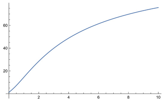
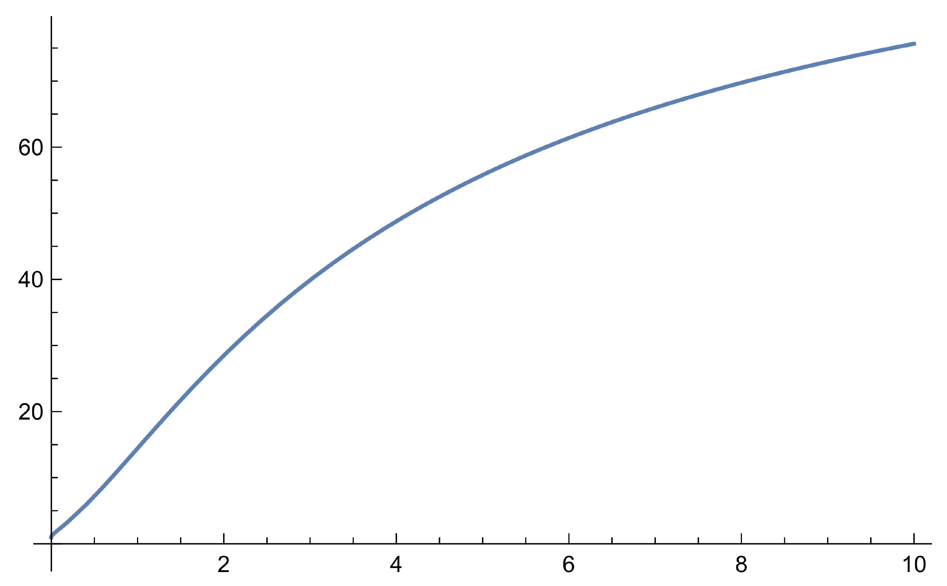
Note the solution of the fractional equation without any impulses ${}_0{}^C\mathcal{D}_{\vartheta \left(t\right)}^{0.5}y\left(t\right)=2y\left(t\right),t>0$ is $y\left(t\right)=x_0{E}_{0.5}\left(2{\left({\displaystyle \frac{t}{t+1}}\right)}^{0.5}\right)$ and it is an increasing function without any bound (see the graph of the function with $x_0=1$ on Figure 1), i.e., it is not stable.

The presence of the impulses in (37) causes a significant influence on the behavior of the solution.

The solution of (37) is given by

$$\begin{array}{c}\hfill x(t;x_0,\left\{{\tau }_k\right\})=\left\{\begin{array}{c}{x}_0{E}_{0.5}\left(2{\left({\displaystyle \frac{t}{t+1}}\right)}^{0.5}\right)for0<t\le {\varsigma }_1,\hfill \\ x_0\sqrt{{\displaystyle \frac{0.5}{E_{0.5}\left(4\right)}}}{E}_{0.5}\left(2{\left({\displaystyle \frac{{\varsigma }_1}{{\varsigma }_1+1}}\right)}^{0.5}\right)E_{0.5}(2\left({({\displaystyle \frac{t}{t+1}}-{\displaystyle \frac{{\varsigma }_1}{{\varsigma }_1+1}})}^{0.5}\right)\hfill \\ for{\varsigma }_1<t\le {\varsigma }_2,\hfill \\ x_0{\displaystyle \frac{0.5}{E_{0.5}\left(4\right)}}{E}_{0.5}\left(2{\left({\displaystyle \frac{{\varsigma }_1}{{\varsigma }_1+1}}\right)}^{0.5}\right)E_{0.5}\left(2\left({({\displaystyle \frac{{\varsigma }_2}{{\varsigma }_2+1}}-{\displaystyle \frac{{\varsigma }_1}{{\varsigma }_1+1}})}^{0.5}\right)E_{0.5}\right(2\left({({\displaystyle \frac{t}{t+1}}-{\displaystyle \frac{{\varsigma }_2}{{\varsigma }_2+1}})}^{0.5}\right)for{\varsigma }_1<t\le {\varsigma }_2\hfill \\ x_0{\left(\sqrt{{\displaystyle \frac{0.5}{E_{0.5}\left(4\right)}}}\right)}^3{E}_{0.5}\left(2{\left({\displaystyle \frac{{\varsigma }_1}{{\varsigma }_1+1}}\right)}^{0.5}\right)E_{0.5}\left(2\left({({\displaystyle \frac{{\varsigma }_2}{{\varsigma }_2+1}}-{\displaystyle \frac{{\varsigma }_1}{{\varsigma }_1+1}})}^{0.5}\right)E_{0.5}\right(2\left({({\displaystyle \frac{t_3}{t+1}}-{\displaystyle \frac{{\varsigma }_3}{{\varsigma }_3+1}})}^{0.5}\right),\hfill \\ for{\varsigma }_2<t\le {\varsigma }_3,\hfill \\ \dots \dots \dots \dots \dots \dots \dots \hfill \end{array}\right.\end{array}$$

(38)

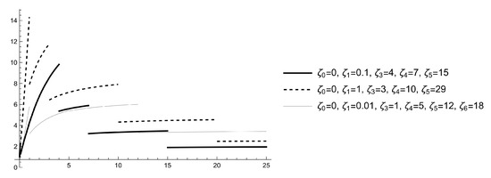
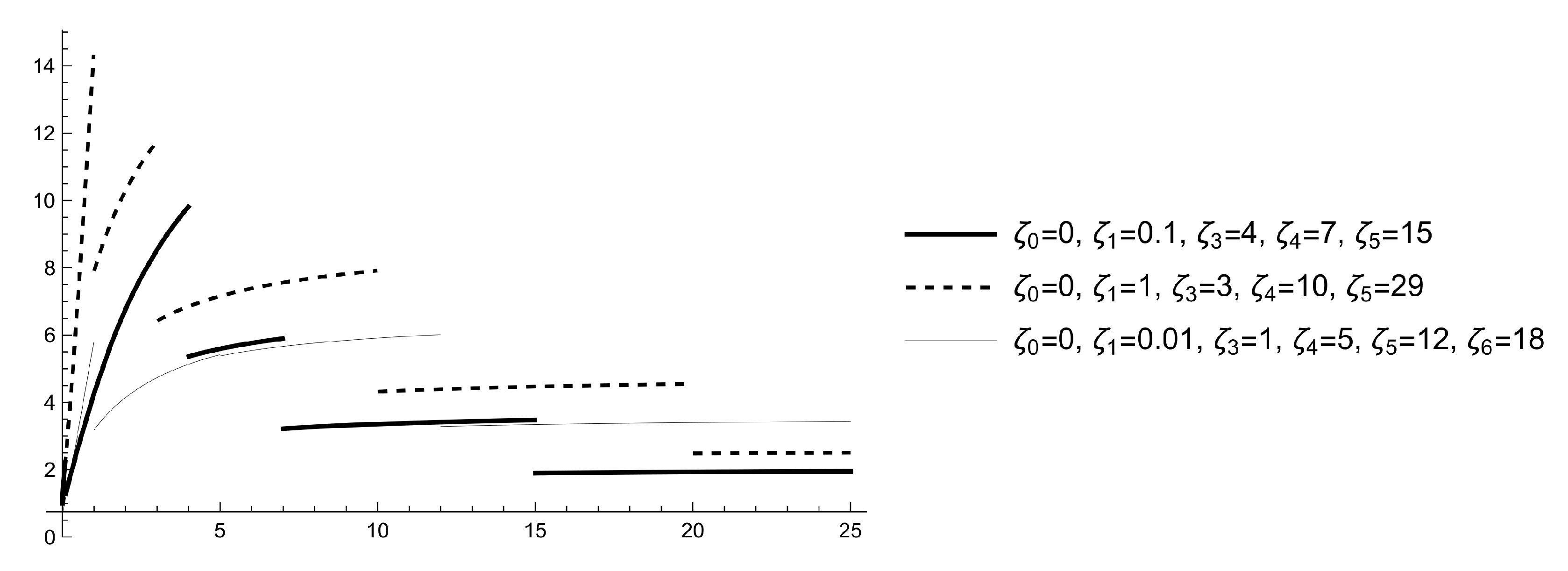
The graphs of some sample path solutions of (37) with $x_0=1$ and different values for the random variables ${\varsigma }_k$ are given in Figure 2.

Consider the Lyapunov function $V\left(x\right)=x^2$. Condition 5(i) of Theorem 2 is satisfied for $p=2$, $a=0.5, b=1$. Condition 5(iii) holds because

$$V\left({\mathcal{I}}_k\left(x\right)\right)={\left(\sqrt{{\displaystyle \frac{0.5}{E_{0.5}\left(4\right)}}}x\right)}^2<0.5x^2=0.5V(x,y).$$

Condition 2 of Theorem 2 is satisfied with $\mathcal{K}=1$.

Let $x(t;x_0,\left\{{\tau }_k\right\})$ be a solution for (37). Consider its arbitrary sample path $x(t;x_0,\left\{{{\rm Y}}_k\right\})$. Then, we obtain

$$\begin{array}{cc}\hfill & {}_{{\eta }_k}{}^C\mathcal{D}_{\vartheta \left(t\right)}^{\delta }V\left(x(t;x_0,\left\{{{\rm Y}}_k\right\})\right)={}_{{\eta }_k}{}^C\mathcal{D}_{\vartheta \left(t\right)}^{\delta }x{(t;x_0,\left\{{{\rm Y}}_k\right\})}^2\le 2{}_{{\eta }_k}{}^C\mathcal{D}_{\vartheta \left(t\right)}^{\delta }x(t;x_0,\left\{{{\rm Y}}_k\right\}))x(t;y_0,\left\{{{\rm Y}}_k\right\})\hfill \\ \hfill & \le 4x^2(t;x_0,\left\{{{\rm Y}}_k\right\}))=4V\left(x(t;y_0,\left\{{{\rm Y}}_k\right\})\right).\hfill \end{array}$$

Therefore, the condition 5(ii) of Theorem 2 is satisfied with $m=4$ for $t>0$.

Also,

$$\begin{array}{cc}& \sum _{k=0}^{\infty }{C}^k{\left(E_{\delta }\left(m{\mathcal{K}}^{\delta }\right)\right)}^{k+1}\sum _{j={\sum }_{i=1}^k{\alpha }_i}^{{\sum }_{i=1}^{k+1}{\alpha }_i-1}{\displaystyle \frac{{\left(\lambda t\right)}^j}{j!}}=\sum _{k=0}^{\infty }{\left({\displaystyle \frac{1}{2E_{0.5}\left(4\right)}}\right)}^k{\left(E_{0.5}\left(4\right)\right)}^{k+1}\sum _{j=2k}^{2k+1}{\displaystyle \frac{{\left(\lambda t\right)}^j}{j!}}\hfill \\ \hfill & =E_{0.5}\left(4\right)\sum _{k=0}^{\infty }{\displaystyle \frac{1}{2^k}}\sum _{j=2k}^{2k+1}{\displaystyle \frac{{\left(\lambda t\right)}^j}{j!}}=E_{0.5}\left(4\right)\left(\sum _{k=0}^{\infty }{\displaystyle \frac{{\left(\lambda t\right)}^{2k}}{2^k\left(2k\right)!}}+\sum _{k=0}^{\infty }{\displaystyle \frac{{\left(\lambda t\right)}^{2(k+1)}}{2^k(2k+1)!}}\right)\hfill \\ \hfill & \le E_{0.5}\left(4\right)\left(\sum _{j=0}^{\infty }{\displaystyle \frac{{\left(\sqrt{0.5}\lambda t\right)}^j}{\left(j\right)!}}+\sqrt{0.5}\sum _{j=1}^{\infty }{\displaystyle \frac{{\left(\sqrt{2}\lambda t\right)}^j}{j!}}\right)\hfill \\ \hfill & =E_{0.5}\left(4\right)(1-\sqrt{0.5})\sum _{j=0}^{\infty }{\displaystyle \frac{{\left(\sqrt{0.5}\lambda t\right)}^j}{\left(j\right)!}}-\sqrt{0.5}\le E_{0.5}\left(4\right)(1-\sqrt{0.5})e^{\sqrt{0.5}\lambda t},\hfill \end{array}$$

(39)

i.e., condition 6 of Theorem 2 holds with $M=E_{0.5}\left(4\right)(1-\sqrt{0.5})>0$ and $\mu =\sqrt{0.5}\lambda <\lambda$.

According to Theorem 2, the zero solution is 2-moment exponentially stable, i.e.,

$$E\left[x{(t;x_0,\left\{{\tau }_k\right\})}^2\right]<x_0^2{E}_{0.5}\left(4\right)(1-\sqrt{0.5})e^{-(1-\sqrt{0.5})\lambda t},t>0.$$

8. Conclusions

Differential equations with Caputo fractional derivatives with respect to other functions and impulses are studied. The main purpose of this study is the application of random variables measuring the time between two consecutive impulses in the studied problem. These random variables are Erlang distributed. The type of applied distribution has a huge influence on the properties of the solutions. First, the detailed explanation of the solutions for the given problem as a stochastic process is given and, second, the p-moment stability properties are investigated. The main study is based on the application of Lyapunov functions. The obtained sufficient conditions depend not only on the nonlinear function and the impulsive functions, but also on the type of applied function in the fractional derivative (see Remark 4) and the distribution of the random variable. Also, it is shown in an example that the presence of random impulses with Erlang distribution significantly change the behavior of the solution. This allows us to use them appropriately for modeling the real-world phenomena and processes.

The above ideas could be applied to study the stability properties of nonlinear differential equations with other types of fractional derivatives. Also, other types of random variables describing the waiting time, such as Gauss distribution, could be applied. This will significantly alter the sufficient conditions and may lead to more suitable models for describing the processes.

In future research, we will try apply the studied nonlinear differential equations to some models.

References

- Iwankiewicz, R. Dynamical Mechanical Systems Under Random Impulses; Advances in Mathematics for Applied Sciences Series; World Scientific: Singapore, 1995. [Google Scholar]
- Boudaoui, A.; Caraballo, T.; Ouahab, A. Stochastic differential equations with non-instantaneous impulses driven by a fractional Brownian motion. Discr. Cont. Dynam. Syst. B 2017, 22, 2521–2541. [Google Scholar] [CrossRef]
- Sanz-Serna, J.M.; Stuart, A.M. Ergodicity of dissipative differential equations subject to random impulses. J. Diff. Equ. 1999, 155, 262–284. [Google Scholar] [CrossRef]
- Wu, H.; Sun, J. p-Moment Stability of Stochastic Differential Equations with impulsive jump and Markovian switching. Automatica 2006, 42, 1753–1759. [Google Scholar] [CrossRef]
- Yang, J.; Zhong, S.; Luo, W. Mean square stability analysis of impulsive stochastic differential equations with delays. J. Comput. Appl. Math. 2008, 216, 474–483. [Google Scholar] [CrossRef]
- Shen, L.; Sun, J. p-th moment exponential stability of stochastic differential equations with impulse effect. Sci. China Inf. Sci. 2011, 54, 1702–1711. [Google Scholar] [CrossRef]
- Agarwal, R.; Hristova, S.; O’Regan, D.; Kopanov, P. Differential equations with random Gamma distributed moments of non-instantaneous impulses and p-moment exponential stability. Demonstr. Math. 2018, 51, 151–170. [Google Scholar] [CrossRef]
- Agarwal, R.P.; Hristova, S.; O’Regan, D.; Kopanov, P. P-moment exponential stability of differential equations with random impulses and the Erlang distribution. Mem. Diff. Equ. Math. Phys. 2017, 70, 99–106. [Google Scholar] [CrossRef]
- Wu, S.; Hang, D.; Meng, X. p-Moment Stability of Stochastic Equations with Jumps. Appl. Math. Comput. 2004, 152, 505–519. [Google Scholar] [CrossRef]
- Almeida, R. A Caputo fractional derivative of a function with respect to another function. Commun. Nonl. Sci. Numer. Simul. 2017, 44, 460–481. [Google Scholar] [CrossRef]
- Feckan, M.; Danca, M.-F.; Chen, G. Fractional Differential Equations with Impulsive Effects. Fractal Fract. 2024, 8, 500. [Google Scholar] [CrossRef]
- Wang, Q.; Lu, D.; Fang, Y. Stability analysis of impulsive fractional differential systems with delay. Appl. Math. Lett. 2015, 40, 1–6. [Google Scholar] [CrossRef]
- Benchohra, M.; Berhoun, F. Impulsive fractional differential equations with variable times. Comput. Math. Appl. 2010, 59, 1245–1252. [Google Scholar] [CrossRef]
- Kucche, K.D.; Kharade, J.P.; da Sousa, J.V.C. On the nonlinear impulsive Ψ–Hilfer fractional differential equations. Math. Modell. Anal. 2020, 25, 642–660. [Google Scholar] [CrossRef]
- Ahmad, B.; Sivasundaram, S. Existence results for nonlinear impulsive hybrid boundary value problems involving fractional differential equations. Nonlinear Anal. Hybrid Syst. 2009, 3, 251–258. [Google Scholar] [CrossRef]
- Benchohra, M.; Slimani, B.A. Existence and uniqueness of solutions to impulsive fractional differential equations. Elect. J. Diff. Equ. 2009, 10, 1–11. [Google Scholar]
- Wang, G.; Ahmad, B.; Zhang, L.; Nieto, J. Comments on the concept of existence of solution for impulsive fractional differential equations. Commun. Nonlinear Sci. Numer. Simulat. 2014, 19, 401–403. [Google Scholar] [CrossRef]
- Zhang, S.; Jiang, W. The existence and exponential stability of random impulsive fractional differential equations. Adv. Differ. Equ. 2018, 404. [Google Scholar] [CrossRef]
- Jose, S.A.; Bose, C.S.V.; Biju, B.P.; Thomas, A. A study on the mild solution of special random impulsive fractional differential equations. Math. Appl. Sci. Eng. 2022, 3, 200–279. [Google Scholar] [CrossRef]
- Wu, S. The Euler scheme for random impulsive differential equations. Appl. Math. Comput. 2007, 191, 164–175. [Google Scholar] [CrossRef]
- Agarwal, R.; Hristova, S.; O’Regan, D. p-Moment exponential stability of Caputo fractional differential equations with noninstantaneous random impulses. J. Appl. Math. Comput. 2017, 55, 149–174. [Google Scholar] [CrossRef]
- Hristova, S.; Ivanova, K. Caputo Fractional Differential Equations with Non-Instantaneous Random Erlang Distributed Impulses. Fractal Fract. 2019, 3, 28. [Google Scholar] [CrossRef]
Disclaimer/Publisher’s Note: The statements, opinions and data contained in all publications are solely those of the individual author(s) and contributor(s) and not of MDPI and/or the editor(s). MDPI and/or the editor(s) disclaim responsibility for any injury to people or property resulting from any ideas, methods, instructions or products referred to in the content. |
© 2024 by the authors. Licensee MDPI, Basel, Switzerland. This article is an open access article distributed under the terms and conditions of the Creative Commons Attribution (CC BY) license (https://creativecommons.org/licenses/by/4.0/).