Abstract
A discrete time modeling method is employed in this paper to analyze and evaluate the reliability of a discrete time K/N: G repairable retrial system with Bernoulli shocks and two-stage repair. Lifetime and shocks are two factors that lead to component failure, and both of them can lead to the simultaneous failure of multiple components. When the repairman is busy, the newly failed component enters retrial orbit and retries in accordance with the first-in-first-out (FIFO) rule to obtain the repair. The repairman provides two-stage repair for failed components, all of which require basic repair and some of which require optional repair. The discrete PH distribution controls the repair times for two stages. Based on discrete time stochastic model properties, priority rules are defined when multiple events occur simultaneously. The state transition probability matrix and state set analysis are used to evaluate the system performance indexes. Numerical experiments are used to illustrate the main performance indexes of the developed discrete time model, and the impact of each parameter variation on the system indexes is examined.
MSC:
90B25; 62N05
1. Introduction
The system will inevitably be subjected to shocks during operation, which may be caused by external friction, collision or over-pressure. The shock model was first proposed and studied by Esary et al. [1]. Subsequently, the shock model has been extensively studied. Shock models can be broadly categorized into four traditional types based on shock failure mechanisms: cumulative [2,3,4], run [5,6], [7,8] and extreme [9,10] shock models. In reliability design, redundancy technology is generally used to improve system reliability. Standby redundancy means that one or more online components work and the redundant components are used as standby components. The standby component replaces the failed component and starts working when an online working component fails. As a means of redundancy, the K/N structure can greatly improve system reliability, which is suitable for various fields such as electronics and military and aerospace design. Research on K/N systems has mainly focused on the assumption that the components have a continuous lifetime distribution [11,12,13,14,15,16].
Systems with discrete lifetime components are widely used in real-world production. For example, the service lifetime of a car tire is measured in kilometers or days and the lifetime of a switch is measured by the number of switches. In reliability studies of discrete time repairable systems, the geometric distribution is often used to model the event occurrence time. However, the disadvantage of applying a geometric distribution is that it reduces the applicability of the model. Once some random variables follow other distributions, it is difficult to analyze the stochastic model, especially to obtain specific analytical results. In view of this phenomenon, the PH distribution was proposed by Neuts, and the properties of the PH distribution and its application in queuing theory were discussed in [17]. In fact, the PH distribution is able to model systems with multiple performance stages in the form of well-structured matrices and is widely used in telecommunications, finance, reliability, biometrics and queuing theory. In addition, since the distribution obeyed by any non-negative random variable can be approximated by the PH distribution, the application of the PH distribution makes the model more general. In recent years, discrete time system models involving discrete PH distribution have been widely studied. Refs. [18,19,20] studied discrete time cold standby systems, in which the lifetime and repair time of the component are both discrete PH distributions. The reliability of the discrete time warm standby repairable system affected by external shocks has been studied in [21,22], where the shock arrival interval follows a discrete PH distribution. Ruiz-Castro and Li [23] conducted reliability modeling for a discrete time K/N: G system with R repairmen, in which component lifetime and repair time are subject to a discrete PH distribution. Based on the properties of the discrete PH distribution, Ruiz-Castro [24] analyzed the discrete time reliability model with preventive maintenance.
In recent years, retrial systems have been widely studied due to their applications in computer networks, telephone communication centers and industrial engineering. Almási et al. [25] studied repairable retrial queueing systems with an unreliable server. The finite-source retrial system with multiple servers and unreliable servers was studied by Gharbi and Ioualalen [26]. Boualem et al. [27] modeled and analyzed an M/G/1 retrial queuing system with vacation. Gao and Wang [28] studied the M/G/1 retrial queuing system with non-persistent customers. Peng et al. [29] considered an M/G/1 retrial G-queue with linear retrial policy, preemptive resume priority, collisions and server breakdowns. Kuo et al. [30] investigated a mixed standby retrial system and performed a cost–benefit ratio analysis for the system with and without retrial. The reliability model of retrial systems with warm standby components and imperfect coverage was studied by Yen and Wang [31]. Wang et al. [32] compared reliability indexes for four retrial systems with unreliable repair equipment and preventive maintenance. For more recent research on retrial systems, see [33,34,35,36].
In most repairable system reliability studies, it is generally assumed that the repairmen only perform one stage of repair on failed components. However, in order to meet different industrial needs, the repair strategy for failed components is diversifying beyond a single phase of repair. Two-stage repair is a common repair strategy with potential applications in communication networks, computer networks, manufacturing systems, and service industries. The early literature mainly focuses on queuing models with two-stage service from the perspective of queuing theory. For example, references [37,38,39] studied the M/G/1 queuing model with a second optional service. Wang and Zhao [40] proposed a discrete time retrial queuing system model with a second optional service and starting failures. Kumar and Jain [41] studied the unreliable queuing model with two-stage service and vacation, and used PSO and ABC optimization algorithms to determine the optimal service rate at optimum cost. Recently, the two-stage repair model from the perspective of system reliability has been studied in the following literature. A warm standby system with a second optional repair service was studied by Gao [42]; the system reliability indexes were solved based on the Laplace transform. Wang et al. [43] studied a linear continuous K/N: F system with vacation and two-stage repair, in which the two-stage repair times obeyed a continuous PH distribution.
Based on the current research status of the K/N: G system, it can be found that the research about the K/N: G system has the following limitations: (1) Shock models for K/N: G systems are generally studied in the continuous case. However, due to the internal structure of the system, working mode and monitoring methods, not all systems can be continuously monitored. (2) In the study of K/N: G system reliability, most K/N: G system models consider a single one-stage repair strategy. However, the case of repairmen providing multiple repair services of multi-stage for failed components is more realistic to research. In view of the above situation, we constructed a shock model of the K/N: G retrial system with two-stage repair in discrete time. The failure of components is influenced by external shocks and their lifetime, both of which might result in several components failing at once. For discrete time K/N: G retrial systems, Yu et al. [44] considered a model with single-stage repair and Bernoulli shocks, where repair time followed a geometric distribution. However, to meet different industrial needs, different repair strategies are often adopted, and additional tasks are assigned to repairmen to reduce the waste of resources. Therefore, based on this model, we extended the single-stage repair system to a two-stage repair system. Repair time was generalized from a geometric distribution to a discrete PH distribution to make the model more general. In addition, a discrete-time K/N: G system model is also discussed in [45], but there are still some significant differences from the model developed in this paper: (1) This paper considers the two-stage repair of repairmen, which was not considered in the work in [45]. (2) Extreme shock is considered in our model, while -shock was considered in [45]. (3) This paper assumes that a discrete PH distribution dominates the repair time of the two stages, which is different from the geometric distribution of repair time in [45].
Based on the above motivation and comparative analysis, the main research work and contributions of this paper are as follows: (1) A shock model for a discrete time K/N: G repairable retrial system with a two-stage repair is proposed based on discrete time stochastic process theory. Both shock and lifetime could lead to simultaneous failure of multiple components. (2) The repairman provides two-stage repair for failed components: basic repair and optional repair. The repair time of both stages is subject to a discrete PH distribution. (3) The sequencing rules for multiple events occurring simultaneously are proposed. Reliability indexes for the system under transient-state and steady-state conditions are analyzed. The rest of this paper is organized as follows. In Section 2, detailed model assumptions and analysis are given. In Section 3, the steady-state and transient-state analyses of the model are performed, and a series of reliability indexes are obtained. The developed model is analyzed numerically in Section 4. Section 5 summarizes this paper.
2. System Model
2.1. Model Description
The system consists of the same independent components; if which K or more components work, the system will work normally. At = 0, all components are new and the repairman is in idle state. When the system is in a failed state, the normal components will still fail. In order to describe the system more intuitively, Figure 1 shows the specific operation principle of the system, and the specific assumptions are as follows:
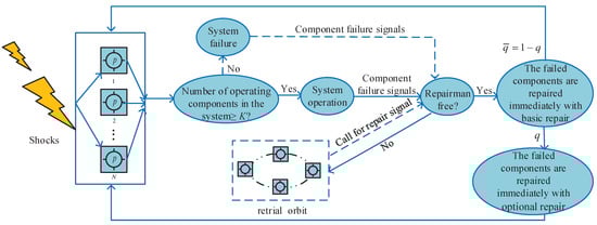
Figure 1.
Operation diagram of a K/N: G retrial system with shock and two-stage repair.
- (a)
- Shock environment: The system suffers from Bernoulli shock currents (rate ), and the effect on components is independent. The failure threshold is a constant or a random variable, and the shock magnitude is a random variable. Component failure occurs at the time when the shock magnitude is more than the failure threshold.
- (b)
- Failure mechanism: The components fail due to two factors: external shocks and their lifetime. These two factors could lead to multiple component failures at once. The lifetime of the component is assumed to be geometrically distributed with parameter p. The impact of lifetime upon the components can be ignored when a shock arrives.
- (c)
- Repair mechanism: The failed component is repaired by a repairman who provides a two-stage repair service: basic repair and optional repair. After the completion of the basic repair, the component is repaired in an optional repair with probability q, or leaves the service desk with probability . Repair times for the two stages are different m-order discrete PH distributions, respectively expressed as , , , and , .
- (d)
- Retrial rule: When the repairman is busy, the newly failed component enters the retrial orbit and retries repeatedly to obtain repair according to FIFO rules. The retrial time is geometrically distributed with parameter .
- (e)
- Priority rule: (1) The following order of occurrence is specified when multiple events occur simultaneously: the component failure, the failed component retrial and the repair completion (any stage of repair). (2) The failure information of components is retrieved one by one when multiple components fail simultaneously, and the component retrieved first has priority for repair or joining the retrial orbit.
2.2. Discrete Time Markov Process
- System state analysis
Based on the model assumption, constitutes a discrete time Markov chain. Here,
and
, if the retrial orbit has s components at time , .
In order to simplify system state analysis, the system states are divided into N + 1 macro states based on the number of failed components. Then, the system state space , working state space and failure state space , in which each macro state is described as follows:
- (1)
- : there are no failed components in the system.
- (2)
- : there are s failed components in the system.
- (3)
- : there are N failed components in the system.
- One-step transition probability
Based on assumption (a), the following two cases are considered.
Case I: the shock magnitude is a random variable X subject to an exponential distribution with parameter , and components have a constant failure threshold c.
Under these circumstances, we use and to denote the probability that an individual component does not fail and fails when subjected to a shock, respectively; then, and .
Case II: the shock magnitude is a random variable X subject to distribution and the failure threshold Y is subject to distribution .
Under these circumstances, the probability that shocks lead to a single component failure is when the shock magnitude value is x. Since X is a random variable, is also a random variable on the interval [0,1]. Let and we assume that the probability distribution function of is ; then,
Let denote the failure of components resulting from a shock, and be the probability of occurrence of ; then,
Let denote the probability that the system transitions from state to . Based on the probability discussion and analysis, one-step transition probabilities of system states under cases I and II are shown in Table 1 and Table 2, respectively.

Table 1.
One-step transition probabilities for case I.
Table 2.
One-step transition probabilities for case II.
2.3. Transition Probability Matrix
We divide the state of the system into working state set and failure state set , and the states in each state set have the following arrangement:
, ,
, ,
, ,
where
, ,
, .
According to the above arrangement, one-step transition probability matrices of the states for cases I and II can be represented by the same block matrix L:
The sub-blocks of L are shown in Appendix A.
3. Reliability Indexes
3.1. System Availability and Failure Condition Probability in Transient State
Let be the probability that the system is in state at time , and
be the system state probability vector, where
, .
Then, the system state probability satisfies the following equations:
According to Equation (1), each state probability function in working state sets and can be expressed as
where
with element 1 in row ,
with element 1 in row ,
with element 1 in row .
Further, the following system reliability indexes can be obtained.
- The system transient-state availability
Based on the above state probability function, we can obtain
Furthermore, based on the above derivation and combined with mathematical computation software, the solution of can be realized by Algorithm 1.
| Algorithm 1: Solution of the system transient-state availability |
Input: N, K, m, , , , , , q, , , , , , , Output: System transient-state availability Procedure: 1: Given the the one-step transition probability matrix L and its block matrices; 2: Assign F as an identity matrix of order ; 3: Compute ; 4: Initialize ; 5: Step 1: Compute ; for do 1.1.Update = ; 1.2.Update ; end 6: Step 2: Compute ; for do for do 2.1.Update ; 2.2.Update ; end end 7: Step 3: Compute ; for do for do 3.1.Update ; 3.2.Update ; end end 8: Final step: sum results. . |
- Failure conditional probability in transient state
When the system is in the working state at time , the probability of system failure at the next time is called the failure conditional probability; then, we can obtain
where with element 1 in column , with element 1 in column , with element 1 in column , , .
In addition, based on the above derivation and combined with mathematical computation software, the solution of can be realized by Algorithm 2.
3.2. System Availability and Failure Condition Probability in Steady State
Let the probability of the system being in state in steady state be , and we denote steady-state probability vectors
where
- System availability in steady state
Based on the above steady-state probability vectors, we have
where , .
- Failure condition probability M in steady state
Combined with the analysis in Section 3.1, the conditional probability of system failure under steady state can be represented as
| Algorithm 2: Solution of the system failure conditional probability |
Input: N, K, m, , , , , , q, , , , , , , Output: Failure conditional probability in transient state 1: Given the the one-step transition probability matrix L and its block matrices; 2: Assign F, I and R as identity matrices of order , and respectively; 3: ; 4: ; for do = ; ; ; end 5: ; for do for do ; ; ; end end 6: ; for do for do ; ; ; end end 7: . |
- Steps for solving the steady-state probability vectors and
- (i)
- Establishment of steady-state probability equation
Based on the discrete time analysis method, the following equations can be constructed:
where , .
- (ii)
- Decomposition of steady-state probability equation
By substituting in Section 2.3 into Equation (9), we can obtain
where , , , , and are non-singular matrices.
- (iii)
- Solution of the steady-state probability equation
,
,
,
,
,
is an identical matrix of order , and is an identical matrix of order .
Then, by substituting Equations (17), (18) and Equations (22)–(24) into Equations (10) and (16), respectively, we can solve for . By substituting back into Equations (17), (18) and Equations (22)–(24) to obtain , , , and .
Further, based on the above derivation and combined with mathematical computation software, the solution of steady-state probability vectors , and M can be realized by Algorithm 3.
| Algorithm 3: Solution of steady-state probability vectors , and M |
Input: N, K, m, , , , , q, , , , , , , Output: , , M 1: Obtain the one-step transition probability matrix L and its block matrices; and do the following 2: ; 3: ; 4: ; 5: ; 6: ; ) 7: ; 8: ; 9: ; 10: ; 11: ; 12: ; ; ; ; ; Calculate based on Equation (7) 13: ; Calculate based on Equation (8) 14: for do ; end 15: ; for do ; ; end 16: ; 17: return , , M. |
4. Numerical Example
A discrete time 2/3: G retrial system shock model based on two-stage repair is considered for two cases. Under case I, the parameters p = 0.02, = 0.01 and = 0.9, q = 0.6 are the basic case, the components have a failure threshold with a value of 30 and the shock magnitude follows an exponential distribution, having a parameter of 0.1. Under case II, the parameters p = 0.02, = 0.01 and = 0.9, q = 0.6 are the basic case, the distribution is the same as the distribution , i.e., the follows a uniform distribution. Assuming that the two-stage repair time in both cases follows the two-order discrete PH distribution and , where , , , , , .
Below, the system model is solved by mathematical computation software and some numerical experimental results are given.
Figure 2 and Figure 3 and Table 3, Table 4 and Table 5 illustrate the influence of each parameter on and for two cases. Figure 2 and Figure 3 and Table 3, Table 4 and Table 5 show that as time increases, gradually decreases and then tends to be stable; gradually increases and then stabilizes. decreases as p and increase, and increases as increases. increases as p and increase and decreases with increasing . As p or increases, the system will be more likely to enter a failed state, which causes to decrease and to increase. As increases, the number of failed components in retrial orbit decreases, which ensures that the system works smoothly for a longer period. This leads to an increase in and a decrease in .
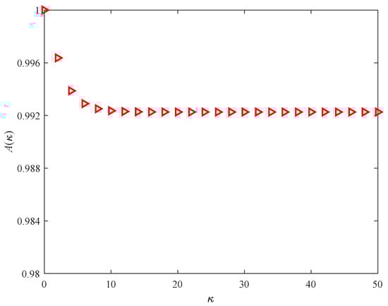
Figure 2.
Variation of with time in case I.
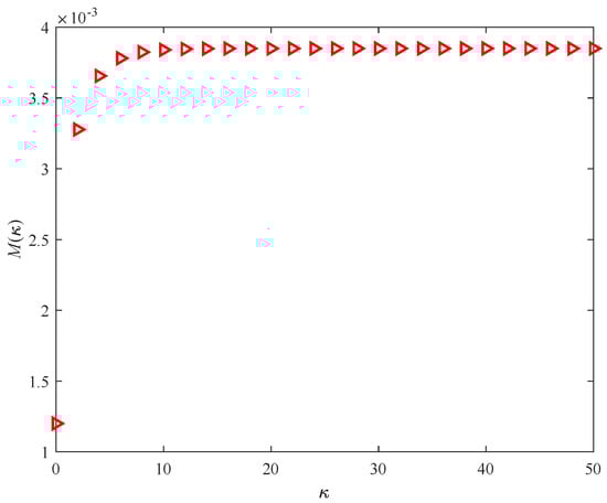
Figure 3.
Variation of with time in case I.
Table 3.
Effect of p for and in case II.
Table 4.
Effect of for and in case II.
Table 5.
Effect of for and in case II.
To further analyze the influence of N values on the system reliability indexes, we performed reliability analysis for a 10/N: G system in case I. The impact of various N for the system indexes is shown in Table 6. The result shows that (1) increases with increasing N. M has the opposite conclusion. (2) It can be seen that adding standby components can significantly improve the system reliability in Table 6. However, when N is greater than 20, the method of adding standby components will no longer be efficient.
Table 6.
10/N: G system reliability indexes.
5. Conclusions
The reliability of some engineering systems needs to be assessed in discrete time, because of their internal structure and operating modes. In view of this, we proposed a shock model of a K/N: G repairable retrial system with two-stage repair in discrete time. The shock arrival interval, component lifetime and retrial time are assumed to be geometrically distributed, and the two-stage repair time is subject to a discrete PH distribution. In order to simplify the calculation and better display the results, the model analysis and main system reliability indexes were presented in matrix form. Based on the discrete time modeling method, the system’s steady-state availability was analyzed by the recurrence method. The transient-state availability and failure conditional probability were evaluated by matrix analysis and state set analysis. The developed system model was demonstrated through numerical experiments, and the variation of the system reliability indexes with the main parameters was analyzed. Additionally, the impact of various N on the system reliability indexes was given.
The reliability shock model developed in this paper has some limitations with respect to the complex and diverse system operation modes and environments. In the future, the model can be deepened in the following aspects: (1) Only one repairman was considered in this study, but in order to be more relevant to real industrial systems, the reliability evaluation of a K/N: G repairable retrial system with multiple repairmen can be considered under the discrete time assumption. (2) In order to model actual engineering systems as accurately as possible, interested scholars can extend this work to discrete time K/N: G repairable retrial systems with mixed standby components. (3) This study considered the extreme shock model and its other shock models can be applied to this model in subsequent studies. (4) The repair of certain components may be abandoned due to high repair costs or severe damage. The failure types of these components should be categorized as non-repairable. Therefore, discrete time K/N: G retrial systems with different failure types can be considered.
Author Contributions
Conceptualization, X.Y. and L.H.; methodology, X.Y.; investigation, Z.H.; writing—original draft preparation, X.Y.; writing—review and editing, L.H. All authors have read and agreed to the published version of the manuscript.
Funding
This work was supported by the National Natural Science Foundation of China [grant number 72071175], Local Science and Technology Development Projects of the Central Committee: S&T Program of Hebei [grant number 246Z0305G], Shijiazhuang Science and Technology Project [grant number 241790737A], and the Basic Innovative Research and Cultivation Project of Yanshan University [grant number 2023LGZD003].
Data Availability Statement
No data were used to support this study.
Conflicts of Interest
The authors declare that they have no known competing financial interests or personal relationships that could have appeared to influence the work reported in this paper.
Appendix A. The Sub-Blocks of the Matrix L
Let
,
,
,
,
,
.
- The transition probability matrices and for the transition of to each state set are as follows:
,
,
,
,
.
- The transition probability matrices and for the transition of to each state set are as follows:
,
,
.
- The transition probability matrices and for the transition of to each state set are as follows:
,
,
,
.
- The transition probability matrices and for the transition of to each state set are as follows:
,
,
,
.
- The transition probability matrices and for the transition of to each state set are as follows:
,
,
- The transition probability matrices and for the transition of to each state set are as follows:
,
,
,
References
- Esary, J.D.; Marshall, A.W.; Proschan, F. Shock models and wear processes. Ann. Probab. 1973, 1, 627–649. [Google Scholar] [CrossRef]
- Gut, A.; Hüsler, J. Realistic variation of shock models. Stat. Probabil. Lett. 2005, 74, 187–204. [Google Scholar] [CrossRef]
- Montoro-Cazorla, D.; Pérez-Ocón, R. A reliability system under cumulative shocks governed by a BMAP. Appl. Math. Model. 2015, 39, 7620–7629. [Google Scholar] [CrossRef]
- Wu, B.; Cui, L.; Yin, J. Reliability and maintenance of systems subject to Gamma degradation and shocks in dynamic environments. Appl. Math. Model. 2021, 96, 367–3812. [Google Scholar] [CrossRef]
- Mallor, F.; Omey, E. Shocks, runs and random sums. J. Appl. Probab. 2001, 38, 438–448. [Google Scholar] [CrossRef]
- Ozkut, M.; Eryilmaz, S. Reliability analysis under Marshall-Olkin run shock model. J. Comput. Appl. Math. 2019, 349, 52–59. [Google Scholar] [CrossRef]
- Eryilmaz, S. δ-shock model based on Polya process and its optimal replacement policy. Eur. J. Oper. Res. 2017, 263, 690–697. [Google Scholar] [CrossRef]
- Lorvand, H.; Nematollahi, A.; Poursaeed, M.H. Life distribution properties of a new δ-shock model. Commun. Stat.-Theor. Methods 2020, 49, 3010–3025. [Google Scholar] [CrossRef]
- Cirillo, P.; Hüsler, J. Extreme shock models: An alternative perspective. Stat. Probabil. Lett. 2011, 81, 25–30. [Google Scholar] [CrossRef]
- Eryilmaz, S.; Kan, C. Reliability and optimal replacement policy for an extreme shock model with a change point. Reliab. Eng. Syst. Saf. 2019, 190, 106513. [Google Scholar] [CrossRef]
- Barron, Y.; Frostig, E.; Levikson, B. Analysis of R out of N systems with several repairmen, exponential life times and phase type repair times: An algorithmic approach. Eur. J. Oper. Res. 2006, 169, 202–225. [Google Scholar] [CrossRef]
- Yuan, L. Reliability analysis for a k-out-of-n: G system with redundant dependency and repairmen having multiple vacations. Appl. Math. Comput. 2012, 218, 11959–11969. [Google Scholar] [CrossRef]
- Zhao, X.; Wu, C.; Wang, S.; Wang, X. Reliability analysis of multi-state k-out-of-n: G system with common bus performance sharing. Comput. Ind. Eng. 2018, 124, 359–369. [Google Scholar] [CrossRef]
- Gao, H.; Cui, L.; Yi, H. Availability analysis of k-out-of-n: F repairable balanced systems with m sectors. Reliab. Eng. Syst. Saf. 2019, 191, 106572. [Google Scholar] [CrossRef]
- Eryilmaz, S.; Devrim, Y. Reliability and optimal replacement policy for a k-out-of-n system subject to shocks. Reliab. Eng. Syst. Saf. 2019, 188, 393–397. [Google Scholar] [CrossRef]
- Wang, X.; Ning, R.; Zhao, X.; Zhou, J. Reliability analyses of k-out-of-n: F capability-balanced systems in a multi-source shock environment. Reliab. Eng. Syst. Saf. 2022, 227, 108733. [Google Scholar] [CrossRef]
- Neuts, M.F. Matrix-Geometric Solutions in Stochastic Models: An Algorithmic Approach; Johns Hopkins University Press: Baltimore, MD, USA, 1981. [Google Scholar]
- Ruiz-Castro, J.E.; Pérez-Ocón, R.; Fernández-Villodre, G. Modelling a reliability system governed by discrete phase-type distributions. Reliab. Eng. Syst. Saf. 2008, 93, 1650–1657. [Google Scholar] [CrossRef]
- Ruiz-Castro, J.E.; Fernández-Villodre, G.; Pérez-Ocón, R. A multi-component general discrete system subject to different types of failures with loss of units. Discrete. Event. Dyn. Syst. 2009, 19, 31–65. [Google Scholar] [CrossRef]
- Kan, C.; Eryilmaz, S. Reliability assessment of a discrete time cold standby repairable system. TOP 2021, 29, 613–628. [Google Scholar] [CrossRef]
- Ruiz-Castro, J.E.; Fernández-Villodre, G. A complex discrete warm standby system with loss of units. Eur. J. Oper. Res. 2012, 218, 456–469. [Google Scholar] [CrossRef]
- Ruiz-Castro, J.E. Complex multi-state systems modelled through marked Markovian arrival processes. Eur. J. Oper. Res. 2016, 252, 852–865. [Google Scholar] [CrossRef]
- Ruiz-Castro, J.E.; Li, Q. Algorithm for a general discrete k-out-of-n: G system subject to several types of failure with an indefinite number of repairpersons. Eur. J. Oper. Res. 2011, 211, 97–111. [Google Scholar] [CrossRef]
- Ruiz-Castro, J.E. Preventive maintenance of a multi-state device subject to internal failure and damage due to external shocks. IEEE Trans. Reliab. 2014, 63, 646–660. [Google Scholar] [CrossRef]
- Almási, B.; Roszik, J.; Sztrik, J. Homogeneous finite-source retrial queues with server subject to breakdowns and repairs. Math. Comput. Model. 2005, 42, 673–682. [Google Scholar] [CrossRef][Green Version]
- Gharbi, N.; Loualalen, M. GSPN analysis of retrial systems with servers breakdowns and repairs. Appl. Math. Comput. 2006, 174, 1151–1168. [Google Scholar] [CrossRef]
- Boualem, M.; Djellab, N.; Aïssani, D. Stochastic inequalities for M/G/1 retrial queues with vacations and constant retrial policy. Math. Comput. Model. 2009, 50, 207–212. [Google Scholar] [CrossRef]
- Gao, S.; Wang, J. Performance and reliability analysis of an M/G/1-G retrial queue with orbital search and non-persistent customers. Eur. J. Oper. Res. 2014, 236, 561–572. [Google Scholar] [CrossRef]
- Peng, Y.; Liu, Z.; Wu, J. An M/G/1 retrial G-queue with preemptive resume priority and collisions subject to the server breakdowns and delayed repairs. J. Appl. Math. Comput. 2024, 44, 187–213. [Google Scholar] [CrossRef]
- Kuo, C.-C.; Sheu, S.-H.; Ke, J.-C.; Zhang, Z.G. Reliability-based measures for a retrial system with mixed standby components. Appl. Math. Model. 2014, 38, 4640–4651. [Google Scholar] [CrossRef]
- Yen, T.-C.; Wang, K.-H. Cost benefit analysis of four retrial systems with warm standby units and imperfect coverage. Reliab. Eng. Syst. Saf. 2020, 202, 107006. [Google Scholar] [CrossRef]
- Wang, K.-H.; Wu, C.-H.; Yen, T.-C. Comparative cost-benefit analysis of four retrial systems with preventive maintenance and unreliable service station. Reliab. Eng. Syst. Saf. 2022, 221, 108342. [Google Scholar] [CrossRef]
- Li, M.; Hu, L.; Wu, S.; Zhao, B.; Wang, Y. Reliability assessment for consecutive-k-out-of-n: F retrial systems under Poisson shocks. Appl. Math. Comput. 2023, 448, 127913. [Google Scholar] [CrossRef]
- Sanga, S.S.; Charan, G.S. Fuzzy modeling and cost optimization for machine repair problem with retrial under admission control F-policy and feedback. Math. Comput. Simulat. 2023, 211, 214–240. [Google Scholar] [CrossRef]
- Kang, J.; Hu, L.; Peng, R.; Li, Y.; Tian, R. Availability and cost-benefit evaluation for a repairable retrial system with warm standbys and priority. Stat. Theory Relat. Fields 2023, 7, 164–175. [Google Scholar] [CrossRef]
- Xu, W.; Li, L.; Fan, W.; Liu, L. Optimal control of a two-phase heterogeneous service retrial queueing system with collisions and delayed vacations. J. Appl. Math. Comput. 2024, 1–28. [Google Scholar] [CrossRef]
- Madan, K.C. An M/G/1 queue with second optional service. Queueing. Syst. 2000, 34, 37–46. [Google Scholar] [CrossRef]
- Wang, J. An M/G/1 queue with second optional service and server breakdowns. Comput. Math. Appl. 2004, 47, 1713–1723. [Google Scholar] [CrossRef]
- Yang, D.-Y.; Wang, K.-H.; Pearn, W.L. Steady-state probability of the randomized server control system with second optional service, server breakdowns and startup. J. Appl. Math. Comput. 2010, 32, 39–58. [Google Scholar] [CrossRef]
- Wang, J.; Zhao, Q. A discrete-time Geo/G/1 retrial queue with starting failures and second optional service. Comput. Math. Appl. 2007, 53, 115–127. [Google Scholar] [CrossRef][Green Version]
- Kumar, A.; Jain, M. Cost optimization of an unreliable server queue with two stage service process under hybrid vacation policy. Math. Comput. Simulat. 2023, 204, 259–281. [Google Scholar] [CrossRef]
- Gao, S. Availability and reliability analysis of a retrial system with warm standbys and second optional repair service. Commun. Stat.-Theor. Methods 2023, 52, 1039–1057. [Google Scholar] [CrossRef]
- Wang, Y.; Hu, L.; Zhao, B.; Tian, R. Stochastic modeling and cost-benefit evaluation of consecutive k/n: F repairable retrial systems with two-phase repair and vacation. Comput. Ind. Eng. 2023, 175, 108851. [Google Scholar] [CrossRef]
- Yu, X.; Hu, L.; Ma, M. Reliability measures of discrete time k-out-of-n: G retrial systems based on Bernoulli shocks. Reliab. Eng. Syst. Saf. 2023, 239, 109491. [Google Scholar] [CrossRef]
- Hu, Z.; Hu, L.; Wu, S.; Yu, X. Reliability assessment of discrete-time k/n (G) retrial system based on different failure types and the δ-shock model. Reliab. Eng. Syst. Saf. 2024, 251, 110371. [Google Scholar] [CrossRef]


Disclaimer/Publisher’s Note: The statements, opinions and data contained in all publications are solely those of the individual author(s) and contributor(s) and not of MDPI and/or the editor(s). MDPI and/or the editor(s) disclaim responsibility for any injury to people or property resulting from any ideas, methods, instructions or products referred to in the content. |
© 2024 by the authors. Licensee MDPI, Basel, Switzerland. This article is an open access article distributed under the terms and conditions of the Creative Commons Attribution (CC BY) license (https://creativecommons.org/licenses/by/4.0/).