Abstract
It is well known that networks are dynamic graphs, and the topology of a network can be described by a graph. Thus, the reliability of a network under edge failure is defined as the probability that its corresponding topological graph remains connected under the condition that the edges fail with independent probabilities. In this paper, the reliability of a class of two-layer networks is considered, where each layer is a complete graph and the edges joining different layers are one-to-one correspondingly connected. The edge failure probability is uniform in the same layer and distinct in different layers and between layers. The recursive formula for the reliability (reliability polynomial) of the two-layer network is obtained, and the corresponding algorithm is also given. Furthermore, the reliability of several networks is computed by Python, which verifies the correctness of the algorithm.
MSC:
68R05; 68R10; 05C31; 05C82
1. Introduction
With the continuous development of science and technology, various networks have interwoven to form an extremely convenient living environment for humans, such as transportation networks, logistics networks, communication networks, and so on [1,2,3]. The nodes or links of these networks may be damaged by different factors [4,5,6], which, in turn, affect the normal operation of the network or even cause network crashes, posing many challenges and inconveniences to people’s work and life. Therefore, network reliability has become an important research direction in the fields of network science, graph theory, and combinatorial mathematics.
However, most network systems do not operate independently but are interconnected in practice. For example, highway, railroad, and aviation networks in transportation systems are interconnected, computer networks and power grids are interdependent, and social networks of different channels influence each other [7,8,9]. In view of this, it has been difficult to meet the practical needs by abstracting various real systems to a single-layer network (single network); therefore, it is extremely necessary to study the reliability of multi-layer networks for the increasingly complex network environments.
As is well known, networks are dynamic graphs, and the topology of a network is described through graphics. In this paper, we no longer distinguish between graphs and networks. So, the reliability of the network is usually transformed into the reliability of the graph. To date, there have been numerous studies on network reliability [10,11,12,13,14,15,16,17,18]. According to the research purposes, these studies are mainly divided into two main areas: reliability analysis [10,11,12,13] and reliability design [14,15,16,17,18].
Based on the number of key nodes, they are further divided into two areas: all-terminal reliability [11,17,18] (connection probability of all vertices of a graph) and k-terminal network reliability [10,12,13,14,15,16] (connection probability of k key vertices in a graph), where with n being the node number of the network.
Indeed, the all-terminal network can be viewed as a single-layer network, while the k-terminal network can be viewed as a multi-layer network. If k key nodes are mutually reachable, the k-terminal network is a two-layer network with a target node layer with k key nodes and a non-target node layer with non-key nodes. In 2021, Xie et al. investigated the problems of uniform optimality [14] for two-terminal graphs and local optimality [15] and uniform optimality [16] for three-terminal graphs, i.e., the optimality problem for two classes of two-layer networks under edge failure with the same probability.
In this paper, we define a class of two-layer networks by the original definition of multi-layer networks [9] and explore their reliability under the condition that the edges fail with independent probabilities. In addition, considering that the link properties between and within each layer in a two-layer network are different, we distinguish the edge failure probabilities unlike most existing studies with the same probability of all edge failures. We obtain a recursive formula for the reliability polynomial of this class of two-layer networks and design a Python algorithm based on this formula to quickly and efficiently output its reliability polynomial by inputting the number of points in each layer of the network and the number of edges between layers.
The two-layer network studied in this paper is fully connected within the layer with only a one-to-one connection between the layers for connecting edges, which is characterized by the full connection of nodes within the layer to achieve efficient information interaction, while the one-to-one connection mode is adopted between the layers to ensure the accuracy of information transfer. Based on the different properties of edges, different failure probabilities are defined to further study their reliability in accordance with the operation characteristics of the real network. This research provides a theoretical basis and research direction for more generalized reliability computation of multi-layer networks. It is also interesting to consider the reliability of two-layer networks with each layer being a complete bipartite graph [19].
This paper is organized as follows. In Section 2, some related basic definitions and notations are given. In Section 3, a recursive formula for the reliability polynomials of a class of two-layer networks is determined. In Section 4, a Python algorithm is designed based on the recursive formula to compute the reliability probabilities of the two-layer network. And we use the Python program to calculate the reliability polynomials for several networks and compare the results with conventional methods in order to double-check the correctness of our recursive formula. Section 5 summarizes the paper.
2. Basic Concepts and Notations
The relevant concepts are listed here, and for other symbols and terminology not explained here, please refer to the book [20]. The probability that the simple graph G remains connected under the condition that the edges fail with independent probabilities q is the reliability of G, denoted by . Conversely, the probability that G is not connected is called the unreliability of G, denoted by . In particular, when and each pair of different vertices in G is connected by an edge, G is called a complete graph with n vertices, denoted by . For a graph H, if and , then H is said to be a spanning subgraph of G. The edge cut of G is the set of edges whose removal leads G to be disconnected. In addition, the degree of the vertex is the number of edges incident with v in the graph G, denoted by .
Based on [9], we define the two-layer network studied in this paper, as follows.
A two-layer network is a pair , where is a family of graphs and is the set of interconnections between nodes of different layers and with .
In this paper, we consider a class of two-layer networks, where , and , which is denoted by .
For convenience, the layer is the first layer and the layer is the second layer of . The vertex set of is
( and ).
And the edge set is containing the following edges
Figure 1 shows the two-layer network .
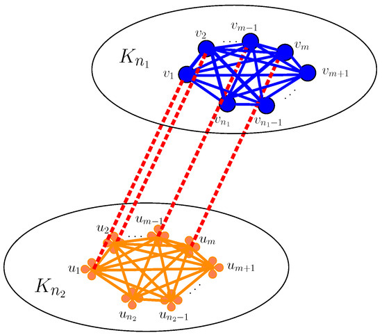
Figure 1.
Two-layer network .
Similar to the reliability definition of a two-terminal network in reference [14], for , and , if , , and are edge failure probabilities for the first layer edges, second layer edges and edges between layers, respectively, then the reliability polynomial of the two-layer network can be written as
where is the number of connected spanning subgraphs of with i edges satisfying edges in the first layer, edges in the second layer, edges between layers, which means that .
And the unreliability polynomial of the two-layer network can be written as
where is the number of edges cut of size i consisting of edges in the first layer, edges in the second layer and edges between layers.
In fact, for smaller networks, we can usually compute the reliability polynomial directly by definition or by the Factorization approach as indicated in the following Lemma.
Lemma 1
([21]). For any edge e in a graph G, the following factorization holds:
where is the graph obtained by identifying the endpoints of edge e in G and is the graph obtained by deleting the edge e from G.
Example 1.
The technical department of a company has two engineers, A and B (complete graph ), and the marketing department has three marketers, C, D, and E (complete graph ). If the probability of successful information transfer between the two engineers is (i.e., the probability of edge failure is ), and the probability of successful message transfer between the three marketers is , and for the purpose of coordinating the project, Engineer A and Marketer Person C need to communicate and the probability of successful message transfer is , then the probability of successful message transfer between all members of these two departments is the reliability polynomial of the two-layer network with edge failure probabilities in the first layer (technology department), in the second layer (marketing department), and for inter-layer edge failures.
If the probability of transmission of information in A and C remains unchanged, and the probability of transmitting information within the technology layer and the market layer is swapped, then the probability of successful transmission of tasks between all members of these two departments is the reliability polynomial of the two-layer network with edge failure probabilities in the first layer (marketing department), in the second layer (technology department), and for inter-layer edge failures.
Figure 2 depicts these two types of two-layer networks, and , with edge failure probabilities in the first layer, in the second layer, and for inter-layer edge failures.
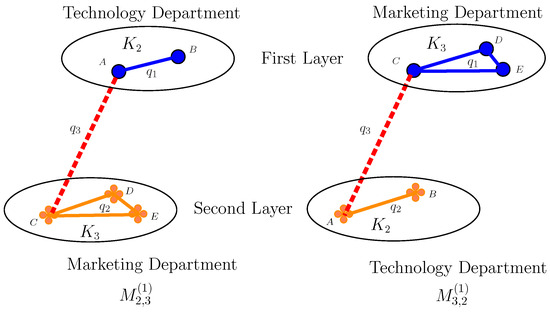
Figure 2.
Graph and .
By Formula , we have
In , the connected spanning subgraphs with edges are three cases, which are , and , so . The connected spanning subgraphs with edges are only , so . Therefore, it can be obtained that
Similarly, we have
In summary, the probability of these two types of cross-sectoral information dissemination networks successfully disseminating information has been obtained. By comparison, it is easy to discover that network reliability varies when different types of edges have differing failure probabilities. Consequently, computing the network reliability polynomial based on different edge failure probabilities is necessary and meaningful. Additionally, we have derived the same result by Lemma 1; the detailed procedure can be found in Appendix B.
However, for larger networks, the number of connected or disconnected spanning subgraphs with i edges is very large, which can easily lead to losing or duplicating some cases during the process of identifying spanning subgraphs. Consequently, the computation of reliability polynomials for networks is NP-hard [11,16].
3. Reliability of Two-Layer Networks
In this section, based on the characteristics of the studied two-layer network, we obtain a recursive formula for the reliability of the two-layer network by analyzing the connected components of the spanning subgraphs, which is described in the following theorem.
To prove the formula, we first introduce a conclusion, which establishes the relationship between the reliability and unreliability polynomials of a two-layer network. Using this relationship, we derive the reliability polynomial of the network through the unreliability polynomial.
Theorem 1.
For the two-layer network , the following equation holds:
Proof.
Obviously, each spanning subgraph of with i edges is either connected or disconnected. Hence, by Formulas (1) and (2), we have
The proof is completed. □
Theorem 2.
The reliability polynomial of the two-layer network satisfies the following recurrence relation:
where ; , , , ; , , ; , .
Proof.
By the definition of graph , it is easy to see that , , and .
For any disconnected spanning subgraph of , there must exist a connected component containing a vertex in the first layer, whose degree is in , without loss of generality, setting this vertex as and this component as C. Let the size of C be i, and there are two cases of C.
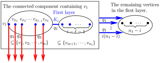
Case 1. The vertex of C is only from the first layer, which means that .
In this case, C consists of , ℓ vertices with degree that are different from , and vertices with degree , as shown in Figure 3.
Figure 3.
C-Case 1, where the red and blue edges with arrows indicate failed edges.
Obviously, . Since there are vertices with degree in the first layer in addition to , there exist ways to select ℓ vertices and . At the same time, there are vertices with degree in the first layer and kinds of selections for the vertices. Obviously, , i.e., . Thus, , . We can see that these two classes of vertices are chosen independently of each other, so the number of such connected components is .
Next, we consider the case of edges in disconnected spanning subgraphs of graph containing connected component C, which is obtained by the following three steps, as shown in Figure 3:
Step 1. The number of edges between C and is and the edge failure probability is , and these edges must fail with probability .
Step 2. The number of edges between vertices with degree in C and the second layer is , and these edges must fail with probability .
Step 3. The reliability of C is equal to the reliability of the complete graph under the condition that the probability of edge failure is , that is, .
Clearly, when the connected component C in this case is determined, the probability of the above disconnected spanning subgraph is . Thus, the probability that any disconnected spanning subgraph of containing C is
Thereby, the sum of the probabilities of all spanning subgraphs in this case is
where .
Case 2.C must have at least one vertex from the second layer, which means that .
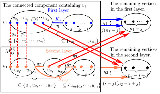
In this case, C consists of , k vertices with degree in the first layer that are different from , vertices with degree in the first layer, r vertices with degree in the second layer and where t is adjacent to t of the vertices with degree from the first layer in this component, and vertices with degree in the second layer, as shown in Figure 4.
Figure 4.
C-Case 2, where the red, blue and orange edges with arrows indicate failed edges.
Obviously, , and . Except for vertex , the selection methods for the other five types of vertices are as follows:
Since there are vertices with degree in the first layer in addition to , there exist ways of selecting k vertices and .
Since there are vertices with degree in the first layer, there exist kinds of selections for the vertices. Obviously, ; then, we have .
Since C is connected, it contains r vertices with degree of the second layer, at least one of which must be adjacent to the vertices with degree selected from the first layer. Hence, and the remaining vertices are chosen among vertices with degree of the second layer. At this point, there are types. It is easy to see that , . Then, we have and .
Since there are vertices with degree in the second layer, there are kinds of selections for the vertices and ; then, we have, .
Thus, , , , and .
Since the vertices in C are selected independently of each other, there are such connected components.
Next, we consider the case of edges in disconnected spanning subgraphs of graph containing connected component C, which is obtained by the following four steps, as shown in Figure 4:
Step 1. The number of edges between j vertices in and the remaining vertices in is , and these edges must fail with probability .
Step 2. The number of edges between vertices in and the remaining vertices in is , and these edges must fail with probability .
Step 3. The number of edges between vertices with degree in and is . In addition, there exist edges between vertices with degree in and . All of these edges must fail with probability .
Step 4. The reliability of C is equal to the reliability of constructed from the first layer , the second layer , and the t edges between the layers, where the probability of an edge failure is in the first layer, in the second layer, and for the edges between layers, that is, .
Clearly, when the connected component C in this case is determined, the probability of the above disconnected spanning subgraph is . Thus, the probability of any disconnected spanning subgraph of containing C is
where , , .
Therefore, the sum of the probabilities of all spanning subgraphs in Case 2 is
where , , , ; , , .
From the above argument, the recurrence relation for the unreliability polynomial of is
where ; , , , ; , , ; , .
Therefore, by Thereom 1, the recurrence relation for the reliability polynomial of is
The proof is completed. □
Especially, the failure probability of all edges in the network is the same, i.e., , the following corollary is obtained.
Corollary 1.
The reliability polynomial of the two-layer network under the condition that all edges fail with probability q satisfies the following recurrence relation:
where ; , , , ; , .
4. The Python Algorithm Based on the Recurrence Formula
Now, based on the recursive formulas established in Theorem 2 and following Lemma 2, we design a Python algorithm to compute the probability of the two-layer network with different edge failure probabilities. We use the Python program to calculate the reliability polynomials for several networks and compare the results with those computed using the Factorization method (Lemma 1), double-verifying the correctness of the recursive formula in Theorem 2.
Lemma 2
([22]). The reliability polynomial of the complete graph , , satisfies the following recurrence relation:
For a two-layer network , if the number of vertices in the first layer, the number of vertices in the second layer, and the number of edges m between the layers are determined, we design a Python algorithm (Algorithm 1) to compute its reliability polynomials as follows.
| Algorithm 1: Python algorithm for computing the reliability polynomials of two-layer networks . |
Initial conditions: For a two-layer network , after determining the values of , and m, perform the following steps.
|
The pseudo-code of the algorithm can be found in Appendix A. In particular, when all edges in the network have the same failure probability, the reliability polynomial of the network based on the edge failure probability of q can be obtained by replacing all , , in the above step with q.
Based on the Python program designed in the above steps, the reliability of several networks is quickly obtained by inputting the number of vertices within the layers and the number of edges between the layers of . Table 1 and Table 2 show the reliability polynomials computed using the Python program for the two-layer network with sizes 5 and 6, respectively, of two cases with different and the same probability of edge failure.

Table 1.
Reliability polynomial of with scale of 5.
Table 2.
Reliability polynomial of with scale of 6.
In addition, we verify several results by the Factorization approach of Lemma 1, see Appendix B.
5. Conclusions
In this paper, we focus on the reliability problem in a class of two-layer networks under conditions where the probability of edge failure differs within different layers and the probability of edge failure between layers is distinct from that within a layer.
We prove the recursive formula for the reliability polynomial of the two-layer network (see Theorem 2), and develop a Python algorithm (see Algorithm 1 or the pseudo-code in Appendix A) based on the formula that efficiently computes the reliability polynomial of the network if the number of vertices in the first layer (), the number of vertices in the second layer () and the number of edges between the layers (m) are determined. Additionally, due to the complexity of the equations, we only list the reliability polynomials for all two-layer networks with scales of 5 and 6. These polynomials have been calculated using the Python program under different edge failure probabilities, and we double-check the correctness of the results by comparing some of them using the Factorization method outlined in Appendix B.
Different from previous studies, based on practical needs, this paper gets rid of the restriction of keeping the network edge failure probability the same and investigates the reliability calculation of a class of two-layer networks under the condition of different edge failure probabilities.
The results and methods of the research enrich the research field of multi-layer network reliability, but we only consider the special two-layer structure with full connectivity within the layers and one-to-one corresponding connectivity between the layers. It is more interesting to continue to study the reliability of the network when the layers are complete bipartite graphs, star graphs, or random graphs and the layers are randomly connected, or to explore the reliability of networks with layers, and the research ideas in this paper provide guidance and direction for further researches.
In addition, Algorithm 1 is obtained based on the recursive formula of Theorem 2; there are 5 loops in the computation process, and there exists an overall call in the inner layer, so the complexity is more than , and reliability polynomials can be obtained efficiently for a certain size of the two-layer network. How to effectively improve the algorithm and reduce time complexity is also an interesting problem.
Author Contributions
Conceptualization, methodology, software, validation, writing—original draft preparation, and writing—review and editing, S.X.; methodology and supervision H.Z.; writing—review, and supervision, J.Y. All authors have read and agreed to the published version of the manuscript.
Funding
This research was funded by the Found of Qinghai Province (Grant No.QHKLYC-GDCXCY-2022-249).
Data Availability Statement
Data are contained within the article.
Conflicts of Interest
The authors declare no conflicts of interest.
Appendix A. Pseudo-Code for Algorithm 1
| Algorithm A1: The calculation of . |
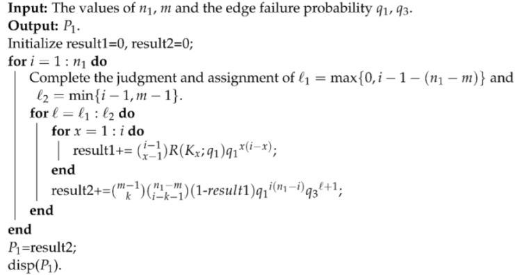 |
| Algorithm A2: The calculation of reliability polynomial of . |
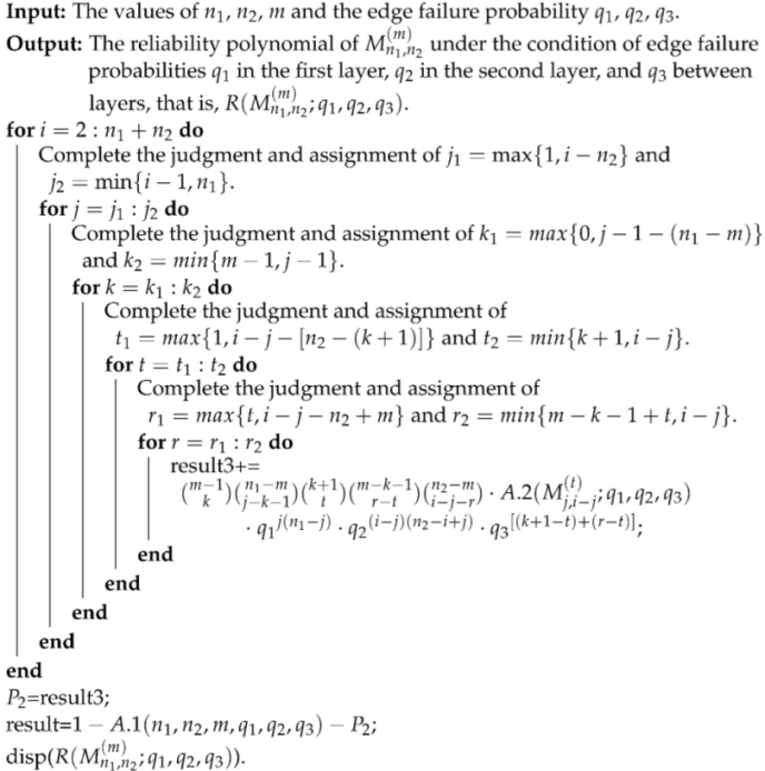 |
Appendix B. The Calculation Process of Reliability Polynomials for Several Two-Layer Networks Using the Factorization Method
Appendix B.1. The Reliability Polynomials , of and
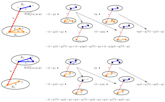
Figure A1.
The process of computing and using the Factorization method.
By calculation, the reliability polynomials of , and are:
Appendix B.2. The Reliability Polynomial of
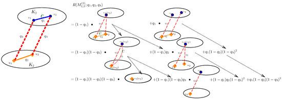
Figure A2.
The process of computing using the Factorization method.
By calculation, the reliability polynomial of is:
Appendix B.3. The Reliability Polynomial of
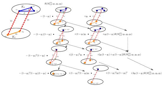
Figure A3.
The process of computing using the Factorization method.
By calculation, the reliability polynomial of is:
Appendix B.4. The Reliability Polynomial of
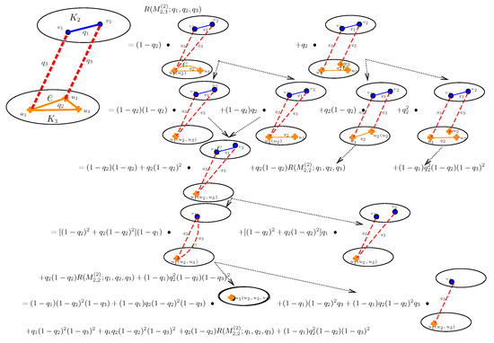
Figure A4.
The process of computing using the Factorization method.
By calculation, the reliability polynomial of is:
References
- Fang, J.Q.; Wang, X.F.; Zheng, Z.G.; Li, X.; Di, Z.R.; Qiao, B. New interdisciplinary science: Network Science(I). Prog. Phys. 2007, 27, 239–343. [Google Scholar]
- Fang, J.Q.; Wang, X.F.; Zheng, Z.G.; Li, X.; Di, Z.R.; Qiao, B. New interdisciplinary science: Network Science(II). Prog. Phys. 2007, 27, 361–448. [Google Scholar]
- Boesch, F.T.; Satyanarayana, A.; Suffel, C. A survey of some network reliability analysis and synthesis results. Networks 2009, 54, 99–107. [Google Scholar] [CrossRef]
- Chen, Y.N.; He, Z.S. Bounds on the reliability of distributed systems with unreliable nodes & links. IEEE Trans. Reliab. 2004, 53, 205–215. [Google Scholar]
- Liu, S.B.; Cheng, K.H.; Liu, X.P. Network reliability with node failures. Networks 2015, 35, 109–117. [Google Scholar] [CrossRef]
- Holme, P.; Kim, B.J. Attack vulnerability of complex networks. Phys. Rev. E 2002, 65, 056109. [Google Scholar] [CrossRef]
- Cardillo, A.; Zanin, M.; Gómez-Gardeñes, J.; Romance, M.; Alejandro, J.; del Amo, G.; Boccaletti, S. Modeling the multi-layer nature of the European Air Transport Network: Resilience and passengers re-scheduling under random failures. Eur. Phys. J. Spec. Top. 2013, 215, 23–33. [Google Scholar] [CrossRef]
- Kivelä, M.; Arenas, A.; Barthelemy, M.; Gleeson, J.P.; Moreno, Y.; Porter, M.A. Multilayer Networks. J. Complex Netw. 2014, 2, 203–271. [Google Scholar] [CrossRef]
- Boccaletti, S.; Bianconi, G.; Criado, R.; del Genio, C.I.; Gómez-Gardeñes, J.; Romance, M.; Sendiña-Nadal, I.; Wang, Z.; Zanin, M. The structure and dynamics of multilayer networks. Phys. Rep. 2014, 544, 1–122. [Google Scholar] [CrossRef]
- Brown, J.; Degagné, C.D.C. Roots of two-terminal reliability polynomials. Networks 2021, 78, 153–163. [Google Scholar] [CrossRef]
- Silva, J.; Gomes, T.; Tipper, D.; Martins, L.; Kounev, V. An effective algorithm for computing all-terminal reliability bounds. Networks 2015, 66, 290. [Google Scholar] [CrossRef]
- Niu, Y.F.; Wang, Y.H.; Xu, X.Z. New decomposition algorithm for computing two-terminal network reliability. Comput. Eng. Appl. 2011, 47, 79–82. [Google Scholar]
- Zhang, H.; Zhao, L.C.; Wang, L.; Sun, H.J. An New Algoirhtm of compuitng K-terminal network reliability. Sicence Technol. Eng. 2005, 5, 387–390. [Google Scholar]
- Xie, S.; Zhao, H.X.; Yin, J. Nonexistence of uniformly most reliable two-terminal graphs. Theor. Comput. Sci. 2021, 892, 279–288. [Google Scholar] [CrossRef]
- Xie, S.; Zhao, H.X.; Dai, L.M.; Yin, J. On locally most reliable three-terminal graphs of sparse graphs. AIMS Math. 2021, 6, 7518–7531. [Google Scholar] [CrossRef]
- Xie, S.; Zhao, H.X.; Yin, J. Uniformly Most Reliable three-terminal Graph of Dense Graphs. Math. Probl. Eng. 2021, 2021, 1–10. [Google Scholar] [CrossRef]
- Brown, J.I.; Cox, D. Nonexistence of optimal graphs for all terminal reliability. Networks 2014, 63, 146–153. [Google Scholar] [CrossRef]
- Archer, K.; Graves, C.; Milan, D. Classes of uniformly most reliable graphs for all-terminal reliability. Discret. Appl. Math. 2019, 267, 12–29. [Google Scholar] [CrossRef]
- Rowshan, Y. The m-bipartite Ramsey number of the K2,2 versus K6,6. Contrib. Math. 2022, 5, 36–42. [Google Scholar]
- Bondy, J.; Murty, U.S.R. Graph Theory; Springer: Berlin/Heidelberg, Germany, 2008. [Google Scholar]
- Satyanarayana, A.; Chang, M.K. Network reliability and the factoring theorem. Networks 1983, 13, 107–120. [Google Scholar] [CrossRef]
- Lange, T.; Reinwardt, M.; Tittmann, P. A recursive formula for the two-edge connected and biconnected reliability of a complete graph. Networks 2017, 69, 408–414. [Google Scholar] [CrossRef]
Disclaimer/Publisher’s Note: The statements, opinions and data contained in all publications are solely those of the individual author(s) and contributor(s) and not of MDPI and/or the editor(s). MDPI and/or the editor(s) disclaim responsibility for any injury to people or property resulting from any ideas, methods, instructions or products referred to in the content. |
© 2024 by the authors. Licensee MDPI, Basel, Switzerland. This article is an open access article distributed under the terms and conditions of the Creative Commons Attribution (CC BY) license (https://creativecommons.org/licenses/by/4.0/).