Finite-Region State Feedback Control for 2-D Switched Systems with Actuator Saturation Under the Weighted Average Dwell Time Technique

Abstract

By using a weighted average dwell time approach, the finite-region stability and stabilization problems are investigated for a class of two-dimensional switched systems with actuator saturation in the Fornasini–Marchesini local state-space model. Firstly, we analyze the finite-region stability of the system studied by introducing the weighted average dwell time approach for the first time. Secondly, the classical state feedback control method is introduced to the system. Based on the established conditions, sufficient criteria are derived to ensure the resulting closed-loop system is finite-region-stable. Finally, a numerical example is provided to show the effectiveness of the provided design approach.

1. Introduction

Two-dimensional (2-D) systems whose states depend on two independent variables, which play an important role in air drying, seismographic data processing, digital signal processing, and so on [1,2], have attracted the attention of many scholars over the past decade. Many essential results of 2-D switched systems have been proposed such as stability analysis [3,4,5,6], $H_{\infty }$ control [7], dissipative control [8,9,10,11], filtering problems [12,13], and fault detection problems [14]. Notably, 2-D switched systems can described by the Roesser model [15], the Fornasini–Marchesini local state-space (FMLSS) model [16], and others. In particular, the Roesser model can be transformed into the FMLSS model. In recent years, some prominent progress has been made in the study of 2-D system stability analysis and controller design. The common methods for analyzing the stability of 2-D switched systems are the average dwell time (ADT) method [17,18,19] and the mode-dependent average dwell time (MDADT) method [20,21]. However, ADT and MDADT methods are two extremes and have their advantages and disadvantages. The former considers the compensation effect between subsystems without considering the differences between them, while the latter considers the differences between subsystems but neglects the compensation effect between them. The weighted average dwell time (WADT) switching technique [22] provides a more flexible method in practice, in which both the differences and compensation effects between subsystems can be considered simultaneously by selecting appropriate weighting coefficients. It is worth noting that for 2-D switched systems, although there have been many studies on Lyapunov asymptotic stability (LAS), there is limited research to analyze finite-region stability (FRS). That is one of the main motivations for the current work.

Due to the existence of hard limitations, actuator saturation is a quite common and inherent phenomenon in the control of many physical systems. The actuator saturation may degrade the system performance, and even lead to system instability. Hence, it is worth noting that from the perspective of practical applications, actuator saturation should be taken into account due to physical, technical, and safety constraints, which usually leads to nonlinear behavior, so it is necessary to discuss the stability of actuator-saturated systems. Therefore, considering actuator saturation in the stabilization of 2-D FMLSS switched systems is a more practical technique. The analyses of Lyapunov stability, finite-time stability, and FRS play an essential role. In recent years, the finite-time stability and stabilization of one-dimensional switched systems have attracted widespread attention [23,24]. The FRS of 2-D switched systems is an extension of the finite-time stability of one-dimension switched systems. Unfortunately, there are few existing studies on the FRS of 2-D switched systems. The concept of FRS and finite-region boundedness (FRB) was initially introduced in [25,26] for 2-D systems. In [25], the authors studied the FRS and FRB of 2-D systems based on the Roesser model, but they did not consider system switching. Subsequently, research on FRS and finite-region dissipativity, along with finite-region dissipative control with missing measurements, has been explored for 2-D systems in studies such as [27,28]. Recently, the novel problems of (input–output) FRS have been first discussed in [29], and the positivity characteristic and the saturation constraint, as well as the switched mechanism, have been taken into account in [30]. In this article, we consider the FRS of 2-D systems affected by switching signals, and it is based on the FMLSS model, which is more general than the Roesser model.

The main contribution of this article is to use the WADT method for the first time to study the finite-region state feedback control problem of 2-D switched systems under saturation constraints and establish sufficient solvability conditions to ensure the FRS of the system.

The rest of this article is organized as follows: In Section 2, the issues to be studied and some necessary preliminaries are provided. Section 3 involves the FRS analysis and finite-region stabilization of 2-D switched systems with actuator saturation using the WADT method. A numerical example is provided to demonstrate the effectiveness of the proposed method in Section 4. Section 5 presents the conclusion of this paper.

The notations used in this paper are shown in the Notation in Nomenclatures section.

2. Problem Statements and Preliminaries

Consider the following system with input saturation described by the FMLSS model:

$$\begin{array}{c}\hfill \begin{array}{cc}\hfill x(s+1,t+1)=& A_{1\rho (s,t+1)}x(s,t+1)+A_{2\rho (s+1,t)}x(s+1,t)+B_{1\rho (s,t+1)}\mathrm{sat}\left(u(s,t+1)\right)\hfill \\ \hfill & +B_{2\rho (s+1,t)}\mathrm{sat}\left(u(s+1,t)\right),\hfill \\ \hfill y(s,t)=& C_{\rho (s,t)}x(s,t),\hfill \end{array}\end{array}$$

(1)

and the input saturation function is defined as follows:

$$\mathrm{sat}\left(u(s,t)\right)={[\mathrm{sat}\left(u_1(s,t)\right),\mathrm{sat}\left(u_2(s,t)\right),\cdots ,\mathrm{sat}\left(u_r(s,t)\right)]}^{\top }:{\mathbb{R}}^r⟶{\mathbb{R}}^r$$

with $\mathrm{sat}\left(u_i(s,t)\right)=min\{1,|u_i(s,t)\left|\right\}\mathrm{sign}\left(u_i(s,t)\right),i=1,2,\cdots ,r$, where $x(s,t)\in {\mathbb{R}}^n$ is the state vector of the system; $y(s,t)\in {\mathbb{R}}^v$ denotes the measured output; and $u(s,t)={[u_1(s,t),u_2(s,t),\cdots ,u_r(s,t)]}^{\top }\in {\mathbb{R}}^r$ represents the input vector. $\rho (s,t):{\mathbb{Z}}_{⊬}\times {\mathbb{Z}}_{⊬}⟶\overline{M}=\{1,2,\cdots ,M\}$ is called a switching signal, where M denotes the number of subsystems. The matrices $A_{1k},A_{2k},B_{1k},B_{2k}$, and $C_k$ are known matrices with appropriate dimensions for $k\in \overline{M}$. To be more specific, from the structural feature of system (1), it is observed that the state values at point $(s+1,t+1)$ are related to those at both $(s,t+1)$ and $(s+1,t)$.

The finite region considered in this paper is a triangular region $Tri\left(N\right)$ defined as follows:

$$Tri\left(N\right)=\{(s,t)\in {\mathbb{Z}}_{⊬}\times {\mathbb{Z}}_{⊬}|s+t\le N\},$$

where N is a given positive integer.

The boundary condition of the 2-D switched system (1) is represented as follows:

$$x_0(s,t)={[x^{\top }(0,t),x^{\top }(s,0)]}^{\top }$$

Define this boundary condition $x_0(s,t)$ within the triangular finite-region $Tri\left(N\right)$ as follows:

$$\begin{array}{c}\hfill x_0(s,t)={[x^{\top }(0,t),x^{\top }(s,0)]}^{\top },(s,t)\in Tri\left(N\right).\end{array}$$

(2)

In this context, condition (2) implies that when $s,t>N$, the following holds: $x(s,0)=x(0,t)\equiv 0$.

It is assumed that the switching only occurs at $s+t$ in this paper. This means that the switching signal $\rho (s,t)$ is solely dependent on the $s+t$. To denote this, we adopt the notation $\rho (s,t)=\rho (s+t)$, that is, $\rho (s,t)=\rho \left(h\right)$ when $s+t=h$. Moreover, we can describe $\rho \left(h\right)$ as $h_q$, $q=1,2,\cdots ,N$, where $s_q+t_q=h_q$$(q=1,2,\cdots ,N)$ represents the $q\text{-}\mathrm{th}$ switching instant. When $\rho \left(h_q\right)=k\in \overline{M}$, it signifies that the $k\text{-}\mathrm{th}$ subsystem is active during the interval $[h_q,h_{q+1})$.

The aim of this paper is to analyze the problem of the finite-region state feedback control for 2-D switched systems with actuator saturation. Before that, we provide some definitions to be used. Firstly, we will introduce the definition of FRS for 2-D switched FMLSS model (1) with $u(s,t)=0$.

Definition 1

([25]). Given a positive integer N, a positive definite matrix Υ, a switching signal $\rho (s,t)$, and positive constants $c_1$, $c_2$ with $c_1<c_2$, the 2-D system (1) with zero control input is said to be finite-region-stable with respect to $(c_1,c_2,N,{\rm Y},\rho (s,t))$, if

$$\begin{array}{c}\hfill x^{\top }(s,t){\rm Y}x(s,t)\le c_2\end{array}$$

(3)

holds for all $s,t\in Tri\left(N\right)$ when the boundary condition given in (2) satisfies

$$\begin{array}{c}\hfill x^{\top }(s,0){\rm Y}x(s,0)+x^{\top }(0,t){\rm Y}x(0,t)\le c_1.\end{array}$$

(4)

Remark 1.

For 2-D switched systems, the FRS and LAS are two distinct definitions. The 2-D switched system could be LAS but not FRS and vice versa. It is significant to notice that these two definitions cannot be mutually inferred. For example, Theorem 3.1 in reference [30] states that the 2-D switched system is FRS, where ${\alpha }_k\ge 1$ indicates that it is not LAS.

Conversely, consider the following system with two subsystems:

$$x(s+1,t+1)=A_{1\rho (s,t+1)}x(s,t+1)+A_{2\rho (s+1,t)}x(s+1,t),$$

where $x(s,t)\in {\mathbb{R}}^1$ is the state vector of the system, and

$$A_{1\rho (s,t)}=A_{2\rho (s,t)}=\left\{\begin{array}{cc}1.3,\hfill & \mathit{if}s+t\in Tri\left(N\right);\hfill \\ 0.47,\hfill & \mathit{if}s+t\notin Tri\left(N\right).\hfill \end{array}\right.$$

Take $c_1=1.1$, $c_2=4$, ${\rm Y}=1$, $N=2$, and then the triangular region is $Tri\left(2\right)=\{(s,t)\in {\mathbb{Z}}_{⊬}\times {\mathbb{Z}}_{⊬}|s+t\le 2\}$. Define this boundary condition as $x_0(s,t)={[x^{\top }(0,t),x^{\top }(s,0)]}^{\top }={[1,1]}^{\top },(s,t)\in Tri\left(2\right)$. When $s,t>2$, the following holds: $x(s,0)=x(0,t)\equiv 0$. As shown in Figure 1, the value of the point (2, 1) in the given triangular region is equal to $4.68>c_2=4$, indicating that the system is not FRS with respect to $(1.1,4,2,{\rm Y}=1,\rho (s,t\left)\right)$. However, after crossing the triangular region, $x(s,t)$ rapidly decreases towards zero, as $s+t$ increases towards $+\infty$; that is, the system is LAS, as shown in Figure 1, but not FRS. The corresponding simulation diagram in the paper uses gradient colors to reflect the three-dimensional effect.

The positive constant ${\tau }_d$ is referred to as the dwell time, satisfying the condition $h_{q+1}-h_q\ge {\tau }_d$ for all $q\in 1,2,\cdots ,N$. This condition ensures that there is a minimum duration between consecutive switching times. We propose the concept of WADT for 2-D switched systems in this paper to obtain more general stability results.

Definition 2.

Let $s_1+t_1={\ell }_1\le s_2+t_2={\ell }_2$. Define $N_{\rho k}({\ell }_1,{\ell }_2)$ as the switching numbers of the $k\text{-}\mathit{th}$ subsystem in $({\ell }_1,{\ell }_2]$. ${\wp }_k({\ell }_1,{\ell }_2)$ can be defined as the total duration that the k-th subsystem remains active within the interval $({\ell }_1,{\ell }_2]$, where $k\in \overline{M}$. If there exist positive numbers $N_{0k}$, ${\tau }_{wa}$, and variable positive scalars ${\tau }_{ak}$,

$$\begin{array}{c}\hfill N_{\rho k}({\ell }_1,{\ell }_2)+N_{0k}\ge {\displaystyle \frac{{\wp }_k({\ell }_1,{\ell }_2)}{{\tau }_{ak}}},\end{array}$$

(5)

$$\begin{array}{c}\hfill \sum _{i=1}^M{\alpha }_i{\tau }_{ai}\le {\tau }_{wa},\end{array}$$

(6)

where ${\alpha }_i\ge 0$ and ${\sum }_{i=1}^M{\alpha }_i=1$; ${\tau }_{wa}$ is called the fast weighted average dwell time, and $N_{0k}$ denotes chatter bounds.

Assumption 1.

Suppose that, for some $\varpi \in {\mathbb{Z}}^{+}$, the signal in the paper satisfies the following inequality:

$$|N_{\rho p}({\ell }_2,{\ell }_1)-N_{\rho q}({\ell }_2,{\ell }_1)|<\varpi ,$$

for all ${\ell }_2\ge {\ell }_1$, $p,q\in \overline{M}$.

Remark 2.

It should be observed that the MDADT method ignores the compensatory interactions among subsystems, which depend on the switching times for the respective subsystems. The WADT considers both the compensatory of subsystems and the differences between subsystems. The weighting coefficients are affected by the switching frequency and the rate of descent of the Lyapunov function [31,32]. In order to reduce computational complexity, we make Assumption 1 to eliminate the influence of switching frequency on the calculation of weighting coefficients. Assumption 1 requires a certain balance in the switching between subsystems, which provides strong conditions for switching but also brings convenience to the design of switching signals.

3. Finite-Region Stability Analysis and Stabilization

In this section, finite-region stability for a 2-D switched system (1) under actuator saturation using the WADT method is discussed. After that, the controller is designed for system (1) to ensure the finite-region stability of the resulting closed-loop system.

3.1. Finite-Region Stability Analysis

This subsection introduces a theorem that establishes a set of sufficient conditions of stability of a 2-D switched system (1) with $u(·,·)=0$.

Theorem 1.

Given positive integer N and scalars ${\varsigma }_k\ge 1$, ${\beta }_k\ge 0$, a positive definite matrix Υ, and two positive scalars $c_1$ and $c_2$ ($c_1<c_2$), consider a 2-D switched system (1) with the boundary condition (4). If there exist matrices $Q_{1k}>0,Q_{2k}>0$ such that, for any $k,l\in \overline{M},k\ne l$,

$$\begin{array}{c}\hfill \left[\begin{array}{cccc}-(1+{\beta }_k)Q_{1k}& 0& {\left(A_{1k}\right)}^{\top }& {\left(A_{1k}\right)}^{\top }\\ \ast & -(1+{\beta }_k)Q_{2k}& {\left(A_{2k}\right)}^{\top }& {\left(A_{2k}\right)}^{\top }\\ \ast & \ast & -{\left(Q_{1k}\right)}^{-1}& 0\\ \ast & \ast & \ast & -{\left(Q_{2k}\right)}^{-1}\end{array}\right]<0,\end{array}$$

(7)

$$\begin{array}{c}\hfill Q_{1k}\le {\varsigma }_k{Q}_{1l},Q_{2k}\le {\varsigma }_k{Q}_{2l},\end{array}$$

(8)

$$\begin{array}{c}\hfill {[{\varsigma }_1{\varsigma }_2\cdots {\varsigma }_M]}^{2N}{e}^{\Omega }<{\lambda }_1{c}_2,\end{array}$$

(9)

$$\begin{array}{c}\hfill \sum _{i=1}^M{\alpha }_i{\tau }_{ai}<{\tau }_{wa}^{*}=-{\displaystyle \frac{2Nln({\varsigma }_1{\varsigma }_2\cdots {\varsigma }_M)+\Omega -ln\left({\lambda }_1{c}_2\right)}{2Nln[(1+{\beta }_1)(1+{\beta }_2)\cdots (1+{\beta }_M)]}},\end{array}$$

(10)

where ${\tau }_{ai}$ stands for ADT of the i-th mode and ${\alpha }_i={\displaystyle \frac{ln(1+{\beta }_i)}{ln[(1+{\beta }_1)(1+{\beta }_2)\cdots (1+{\beta }_M)]}}$, $i\in \overline{M}$. Then, the system (1) with $u(·,·)=0$ exhibits finite-region stability with respect to $(c_1,c_2,N,{\rm Y},\rho (·,·))$, where $\Omega =ln[{\displaystyle \frac{{(1+\overline{\beta })}^{2N}-1}{\underline{\beta }}}M+1]+ln\left({\lambda }_2{c}_1\right)+ln\left[{\overline{\varsigma }}^{M\varpi }{\prod }_{k=1}^M{(1+{\beta }_k)}^{(\varpi +N_{0k}){\tau }_{ak}}\right]$, $\underline{\beta }={min}_{k\in \overline{M}}\left\{{\beta }_k\right\},\overline{\beta }={max}_{k\in \overline{M}}\left\{{\beta }_k\right\}$, ${\lambda }_1={min}_{k\in \overline{M}}\left[{\lambda }_{min}\left({\tilde{Q}}_{1k}\right)+{\lambda }_{min}\left({\tilde{Q}}_{2k}\right)\right]$, ${\lambda }_2={max}_{k\in \overline{M}}[{\lambda }_{max}\left({\tilde{Q}}_{1k}\right)+$${\lambda }_{max}\left({\tilde{Q}}_{2k}\right)]$, ${\tilde{Q}}_{1k}={{\rm Y}}^{-{\displaystyle \frac{1}{2}}}{Q}_{1k}{{\rm Y}}^{-{\displaystyle \frac{1}{2}}}$, ${\tilde{Q}}_{2k}={{\rm Y}}^{-{\displaystyle \frac{1}{2}}}{Q}_{2k}{{\rm Y}}^{-{\displaystyle \frac{1}{2}}}$.

Proof of Theorem 1.

Select the Lyapunov candidate function for 2-D switched system (1) with $u(·,·)=0$ as follows:

$$\begin{array}{c}\hfill V_{\rho \left(h\right)}(s,t)=V_{1\rho \left(h\right)}(s,t)+V_{2\rho \left(h\right)}(s,t),\end{array}$$

(11)

where $V_{1\rho \left(h\right)}=x^{\top }(s,t)Q_{1\rho \left(h\right)}x(s,t),V_{2\rho \left(h\right)}=x^{\top }(s,t)Q_{2\rho \left(h\right)}x(s,t)$.

$$\begin{array}{cc}\hfill & V_k(s+1,t+1)-(1+{\beta }_k)[V_{1k}(s,t+1)+V_{2k}(s+1,t)]\hfill \\ \hfill & =V_{1k}(s+1,t+1)+V_{2k}(s+1,t+1)-(1+{\beta }_k)[V_{1k}(s,t+1)\hfill \\ \hfill & +V_{2k}(s+1,t)]\hfill \\ \hfill & ={\overline{x}}^{\top }(s,t){\Psi }_k\overline{x}(s,t)\hfill \end{array}$$

(12)

with

$$\begin{gathered} \overline{x}(s,t)=\left[\begin{array}{c}x(s,t+1)\\ x(s+1,t)\end{array}\right], \\ {\Psi }_k=\left[\begin{array}{cc}{\left(A_{1k}\right)}^{\top }{Q}_k{A}_{1k}-(1+{\beta }_k)Q_{1k}& {\left(A_{1k}\right)}^{\top }{Q}_k{A}_{2k}\\ \ast & {\left(A_{2k}\right)}^{\top }{Q}_k{A}_{2k}-(1+{\beta }_k)Q_{2k}\end{array}\right], \end{gathered}$$

and $Q_k=Q_{1k}+Q_{2k}$. Using Schur complement to condition (7) produces ${\Psi }_k<0$, which implies that, for any $\overline{x}(s,t)\ne 0$,

$$\begin{array}{c}\hfill V_k(s+1,t+1)<(1+{\beta }_k)[V_{1k}(s,t+1)+V_{2k}(s+1,t)].\end{array}$$

(13)

The total switching number of the switching signal $\rho (·,·)$ on the interval $(0,\ell ]$ is denoted as $N_{\rho }(0,\ell )$. The switching points within this interval are ordered as $h_q,q=1,2,\cdots ,m$, where $h_q$ is defined as $h_q=s_q+t_q$. For any $\ell \in [h_m,h_{m+1})$, suppose that $\rho \left(h\right)=\rho \left(h_m\right)=k\in \overline{M}$; then, one has

$$\begin{array}{cc}\hfill \sum _{s+t=\ell }{V}_{\rho \left(h\right)}(s,t)& =V_k(0,\ell )+V_k(1,\ell -1)+\cdots +V_k(\ell ,0)\hfill \\ \hfill & =V_{1k}(0,\ell )+V_{1k}(1,\ell -1)+\cdots +V_{1k}(\ell ,0)\hfill \\ \hfill & +V_{2k}(0,\ell )+V_{2k}(1,\ell -1)+\cdots +V_{2k}(\ell ,0)\hfill \\ \hfill & <(1+{\beta }_k)\sum _{s+t=\ell -1}{V}_k(s,t)+V_k(\ell ,0)+V_k(0,\ell ).\hfill \end{array}$$

(14)

In view of the boundary condition (4), it is derived that

$$\begin{array}{cc}\hfill V_k(\ell ,0)+V_k(0,\ell )& =V_{1k}(\ell ,0)+V_{2k}(\ell ,0)+V_{1k}(0,\ell )+V_{2k}(0,\ell )\hfill \\ \hfill & =x^{\top }(\ell ,0)Q_{1k}x(\ell ,0)+x^{\top }(\ell ,0)Q_{2k}x(\ell ,0)\hfill \\ \hfill & +x^{\top }(0,\ell )Q_{1k}x(0,\ell )+x^{\top }(0,\ell )Q_{2k}x(0,\ell )\hfill \\ \hfill & \le {\lambda }_2[x^{\top }(0,\ell ){\rm Y}x(0,\ell )+x^{\top }(\ell ,0){\rm Y}x(\ell ,0)]\le {\lambda }_2{c}_1,\hfill \end{array}$$

(15)

and one further obtains

$$\begin{array}{cc}\hfill \sum _{s+t=\ell }{V}_k(s,t)& \le {\lambda }_2{c}_1+(1+{\beta }_k)\sum _{s+t=\ell -1}{V}_k(s,t)\hfill \\ \hfill & \le {\lambda }_2{c}_1+(1+{\beta }_k)[{\lambda }_2{c}_1+(1+{\beta }_k)\sum _{s+t=\ell -2}{V}_k(s,t)]\hfill \\ \hfill & \le \cdots \hfill \\ \hfill & \le {\lambda }_2{c}_1+\cdots +{(1+{\beta }_k)}^{\ell -h_m-1}{\lambda }_2{c}_1+{(1+{\beta }_k)}^{\ell -h_m}\sum _{s+t=h_m}{V}_k((s,t).\hfill \end{array}$$

(16)

From (8), the following inequality holds at every switching instant $h_q,q=1,2,\cdots ,m$.

$$\begin{array}{cc}\hfill \sum _{s+t=h_q}{V}_{\rho \left(h_q\right)}(s,t)& \le {\varsigma }_{\rho \left(h_q\right)}\sum _{s+t=h_q}{V}_{\rho \left(h_{q-1}\right)}(s,t)\hfill \\ \hfill & \le {\varsigma }_{\rho \left(h_q\right)}[{\lambda }_2{c}_1+(1+{\beta }_{\rho \left(h_{q-1}\right)})\sum _{s+t=h_q-1}{V}_{\rho \left(h_{q-1}\right)}(s,t)].\hfill \end{array}$$

(17)

Then, when $h\in [h_{m-1},h_m),\rho \left(h\right)=\rho \left(h_{m-1}\right)=l\in \overline{M}$, the following is derived:

$$\begin{array}{cc}\hfill \sum _{s+t=h_m}{V}_k(s,t)& \le {\varsigma }_k\sum _{s+t=h_m}{V}_l(s,t)\hfill \\ \hfill & \le {\varsigma }_k[{\lambda }_2{c}_1+(1+{\beta }_l)\sum _{s+t=h_m-1}{V}_l(s,t)].\hfill \end{array}$$

(18)

where ${\rho }_q$ represents $\rho \left(h_q\right)$. Combined with (16)–(18), the following expression can be obtained:

$$\begin{array}{cc}\hfill \sum _{s+t=\ell }{V}_{{\rho }_m}(s,t)& \le {\lambda }_2{c}_1+\cdots +{(1+{\beta }_{{\rho }_m})}^{\ell -h_m-1}{\lambda }_2{c}_1\hfill \\ \hfill & +{\varsigma }_{{\rho }_m}{(1+{\beta }_{{\rho }_m})}^{\ell -h_m}\sum _{s+t=h_m}{V}_{{\rho }_{m-1}}(s,t)\hfill \\ \hfill & \le {\displaystyle \frac{{\lambda }_2{c}_1[1-{(1+{\beta }_{{\rho }_m})}^{\ell -h_m}]}{1-(1+{\beta }_{{\rho }_m})}}\hfill \\ \hfill & +{\varsigma }_{{\rho }_m}{(1+{\beta }_{{\rho }_m})}^{\ell -h_m}[{\lambda }_2{c}_1+(1+{\beta }_{{\rho }_{m-1}})\sum _{s+t=h_m-1}{V}_{{\rho }_{m-1}}(s,t)]\hfill \\ & \le \cdots \hfill \\ \hfill & \le {\displaystyle \frac{{(1+{\beta }_{{\rho }_m})}^{\ell -h_m}-1}{{\beta }_{{\rho }_m}}}{\lambda }_2{c}_1+{\varsigma }_{{\rho }_m}{(1+{\beta }_{{\rho }_m})}^{\ell -h_m}{\displaystyle \frac{{(1+{\beta }_{{\rho }_{m-1}})}^{h_m-h_{m-1}}-1}{{\beta }_{{\rho }_{m-1}}}}{\lambda }_2{c}_1\hfill \\ & +\cdots \hfill \\ & +{\varsigma }_{{\rho }_m}\cdots {\varsigma }_{{\rho }_2}{(1+{\beta }_{{\rho }_m})}^{\ell -h_m}\cdots {(1+{\beta }_{{\rho }_2})}^{h_3-h_2}{\displaystyle \frac{{(1+{\beta }_{{\rho }_1})}^{h_2-h_1}-1}{{\beta }_{{\rho }_1}}}{\lambda }_2{c}_1\hfill \\ & +{\varsigma }_{{\rho }_m}\cdots {\varsigma }_{{\rho }_1}{(1+{\beta }_{{\rho }_m})}^{\ell -h_m}\cdots {(1+{\beta }_{{\rho }_1})}^{h_2-h_1}{\displaystyle \frac{{(1+{\beta }_{{\rho }_0})}^{h_1}-1}{{\beta }_{{\rho }_0}}}{\lambda }_2{c}_1\hfill \\ & +{\varsigma }_{{\rho }_m}\cdots {\varsigma }_{{\rho }_1}{(1+{\beta }_{{\rho }_m})}^{\ell -h_m}\cdots {(1+{\beta }_{{\rho }_0})}^{h_1}\sum _{s+t=0}{V}_{{\rho }_0}(s,t).\hfill \end{array}$$

(19)

Due to

$$\begin{array}{cc}\hfill \sum _{s+t=0}{V}_{{\rho }_0}(s,t)& \le \underset{k\in \overline{M}}{max}{V}_k(0,0)=\underset{k\in \overline{M}}{max}{x}^{\top }(0,0)Q_{k}x(0,0)\hfill \\ \hfill & \le {\lambda }_2[x^{\top }(0,0){\rm Y}x(0,0)+x^{\top }(0,0){\rm Y}x(0,0)]\le {\lambda }_2{c}_1,\hfill \end{array}$$

(20)

and based on (19), (5), and Assumption 1, we have

$$\begin{array}{cc}\hfill \sum _{s+t=\ell }{V}_{{\rho }_m}(s,t)& \le \prod _{k=1}^M[{\left({\varsigma }_k\right)}^{N_{\rho k}(0,\ell )}{(1+{\beta }_k)}^{{\wp }_k(0,\ell )}][\sum _{k=1}^M{\displaystyle \frac{{(1+{\beta }_k)}^{{\wp }_k(0,\ell )}-1}{{\beta }_k}}{\lambda }_2{c}_1+{\lambda }_2{c}_1]\hfill \\ & \le \prod _{k=1}^M[{\left({\varsigma }_k\right)}^{{\displaystyle \frac{N_{\rho }(0,\ell )}{M}}+\varpi }{(1+{\beta }_k)}^{{\wp }_k(0,\ell )}][\sum _{k=1}^M{\displaystyle \frac{{(1+{\beta }_k)}^{{\wp }_k(0,\ell )}-1}{{\beta }_k}}{\lambda }_2{c}_1+{\lambda }_2{c}_1]\hfill \\ & \le {\overline{\varsigma }}^{M\varpi }\prod _{k=1}^M[{\left({\varsigma }_k\right)}^{{\displaystyle \frac{N_{\rho }(0,\ell )}{M}}}{(1+{\beta }_k)}^{{\displaystyle \frac{N_{\rho }(0,\ell )}{M}}{\tau }_{ak}+(\varpi +N_{0k}){\tau }_{ak}}]\hfill \\ & [\sum _{k=1}^M{\displaystyle \frac{{(1+{\beta }_k)}^{{\wp }_k(0,\ell )}-1}{{\beta }_k}}{\lambda }_2{c}_1+{\lambda }_2{c}_1]\hfill \\ & \le {\overline{\varsigma }}^{M\varpi }\prod _{k=1}^M{(1+{\beta }_k)}^{(\varpi +N_{0k}){\tau }_{ak}}[\prod _{k=1}^M{\left({\varsigma }_k\right)}^{{\displaystyle \frac{N_{\rho }(0,\ell )}{M}}}{(1+{\beta }_k)}^{{\displaystyle \frac{N_{\rho }(0,\ell )}{M}}{\tau }_{ak}}]\hfill \\ & [\sum _{k=1}^M{\displaystyle \frac{{(1+{\beta }_k)}^{{\wp }_k(0,\ell )}-1}{{\beta }_k}}{\lambda }_2{c}_1+{\lambda }_2{c}_1]\hfill \\ & \le exp\{\sum _{k=1}^M{\displaystyle \frac{N_{\rho }(0,\ell )}{M}}ln{\varsigma }_k+{\displaystyle \frac{N_{\rho }(0,\ell )}{M}}{\tau }_{ak}ln(1+{\beta }_k)+\Omega \}\hfill \\ & \le exp\{{\displaystyle \frac{N_{\rho }(0,\ell )}{M}}[ln({\varsigma }_1\cdots {\varsigma }_M)+\sum _{k=1}^{M}ln(1+{\beta }_k){\tau }_{ak}]+\Omega \},\hfill \end{array}$$

(21)

where $\overline{\varsigma }=max\{{\varsigma }_1,{\varsigma }_2,\cdots ,{\varsigma }_M\}$.

One obtains from (9) that $ln\left({\lambda }_1{c}_2\right)-\Omega -2Nln[{\varsigma }_1{\varsigma }_2\cdots {\varsigma }_M]>0$. For any $k\in \overline{M}$, it follows from condition (10) that

$${\alpha }_1{\tau }_{a1}+\cdots +{\alpha }_M{\tau }_{aM}+{\displaystyle \frac{2Nln({\varsigma }_1\cdots {\varsigma }_M)-ln\left({\lambda }_1{c}_2\right)+\Omega }{2Nln[(1+{\beta }_1)\cdots (1+{\beta }_M)]}}<0,$$

$$2Nln({\varsigma }_1\cdots {\varsigma }_M)+2N{\tau }_{a1}ln(1+{\beta }_1)+\cdots +2N{\tau }_{aM}ln(1+{\beta }_M)<ln\left({\lambda }_1{c}_2\right)-\Omega ,$$

that is,

$${\displaystyle \frac{N_{\rho }(0,\ell )}{M}}[ln({\varsigma }_1\cdots {\varsigma }_M)+{\sum }_{k=1}^{M}ln(1+{\beta }_k){\tau }_{ak}]<ln\left({\lambda }_1{c}_2\right)-\Omega .$$

Then, from above inequalities, we can further easily obtain the following for $(s,t)\in Tri\left(N\right)$:

$$\begin{array}{cc}\hfill & \sum _{s+t=\ell }{x}^{\top }(s,t){\rm Y}x(s,t)\hfill \\ \hfill & \le {\displaystyle \frac{exp\left\{\frac{N_{\rho }(0,\ell )}{M}[ln({\varsigma }_1\cdots {\varsigma }_M)+{\sum }_{k=1}^{M}ln(1+{\beta }_k){\tau }_{ak}]+\Omega \right\}}{{\lambda }_1}}\hfill \\ & \le c_2.\hfill \end{array}$$

(22)

Based on (3) and (4), the 2-D switched system (1) with $u(·,·)=0$ is finite-region-stable with respect to $(c_1,c_2,N,{\rm Y},\rho (·,·))$. The proof is then completed. □

The subsequent theorems are all derived from WADT switching to investigate the finite-region stabilization of a 2-D switched system.

3.2. Finite-Region Stabilization

In this subsection, we design the state feedback controller for the 2-D switched system (1) as follows:

$$\begin{array}{c}\hfill u(s,t)=K_{\rho (s,t)}x(s,t),\end{array}$$

(23)

where $K_{\rho (s,t)}$ represents the feedback gain matrix that requires design.

Here, a set of $r\times r$ diagonal matrices are denoted as $\Delta$, with diagonal elements being either 0 or 1. For example, when $N=2$, it can be expressed as follows:

$$\Delta =\{{\Delta }_1,{\Delta }_2,{\Delta }_3,{\Delta }_4\}=\{\mathrm{diag}\{1,1\},\mathrm{diag}\{1,0\},\mathrm{diag}\{0,1\},\mathrm{diag}\{0,0\}\}.$$

Obviously, $\Delta$ consists of $2^r$ elements, and when ${\Delta }_p\in \Delta ,{\Delta }_p^{-}=I_r-{\Delta }_p$ is also an element in $\Delta$, where $p=1,2,\cdots ,2^r$.

For a matrix $H_k\in R^{r\times n},k\in \overline{M}$, the polyhedral set $\S \left(H_k\right)$ is defined as follows:

$$\begin{array}{c}\hfill \S \left(H_k\right)=\{x(s,t)\in R^n:|H_{k_{\left(i\right)}}x(s,t)|\le 1,i=1,2,\cdots ,r\},\end{array}$$

(24)

where $H_{k_{\left(i\right)}}$ is the $i\text{-}\mathrm{th}$ row of the matrix $H_k,k\in \overline{M}$.

For a positive scalar $\omega$ and a positive definite matrix $\Gamma \in {\mathbb{R}}^{n\times n}$, an ellipsoid $\phi (\Gamma ,\omega )$ is defined as the set of points $x(s,t)\in {\mathbb{R}}^n$ satisfying the condition $x^{\top }(s,t)\Gamma x(s,t)\le \omega$, that is,

$$\phi (\Gamma ,\omega )=\{x(s,t)\in R^n:x^{\top }(s,t)\Gamma x(s,t)\le \omega \}.$$

Lemma 1

([33]). Given $K_k\in {\mathbb{R}}^{r\times n}$ and $H_k\in {\mathbb{R}}^{r\times n}$, for any $x(s,t)\in \S \left(H_k\right)$, we have

$$\mathrm{sat}\left(K_{k}x(s,t)\right)\in \mathrm{co}\{({\Delta }_p{K}_k+{\Delta }_p^{-}{H}_k)x(s,t),p=1,2,\cdots ,2^r\},$$

where $\mathrm{co}·$ is the convex hull.

From the state feedback controller (23), one obtains

$$\begin{array}{c}\hfill \mathrm{sat}\left(u(s,t)\right)\in \mathrm{co}\{({\Delta }_p{K}_{\rho (s,t)}+{\Delta }_p^{-}{H}_{\rho (s,t)})x(s,t),p=1,2,\cdots ,2^r\}.\end{array}$$

(25)

By Lemma 1 and (1), (25), one knows that when $x(s,t)\in \S \left(H_{\rho (s,t)}\right)$, for any $\rho \left(h\right)=k\in \overline{M}$, one can obtain the resulting closed-loop system as follows:

$$\begin{array}{c}\hfill \begin{array}{cc}\hfill x(s+1,t+1)=& {\overline{A}}_{1k}x(s,t+1)+{\overline{A}}_{2k}x(s+1,t)\hfill \\ \hfill y(s,t)=& C_{k}x(s,t),\hfill \end{array}\end{array}$$

(26)

where ${\overline{A}}_{1k}=A_{1k}+B_{1k}(K_k{\Delta }_p+H_k{\Delta }_p^{-}),{\overline{A}}_{2k}=A_{2k}+B_{2k}(K_k{\Delta }_p+H_k{\Delta }_p^{-}),p=1,2,\cdots ,2^r$.

Theorem 2.

Given positive integer N and scalars ${\varsigma }_k\ge 1,{\beta }_k\ge 0$, a positive definite matrix Υ, and two positive scalars $c_1$ and $c_2$ ($c_1<c_2$), consider a 2-D closed-loop system (26) with boundary condition (4). If there exist $K_k,H_k,Q_{1k}>0,Q_{2k}>0,k\in \overline{M}$, such that

$$\begin{array}{c}\hfill \left[\begin{array}{cc}{\left({\overline{A}}_{1k}\right)}^{\top }{Q}_k{\overline{A}}_{1k}-(1+{\beta }_k)Q_{1k}& {\left({\overline{A}}_{1k}\right)}^{\top }{Q}_k{\overline{A}}_{2k}\\ \ast & {\left({\overline{A}}_{2k}\right)}^{\top }{Q}_k{\overline{A}}_{2k}-(1+{\beta }_k)Q_{2k}\end{array}\right]<0,\end{array}$$

(27)

$$\begin{array}{c}\hfill \phi (Q_k,1)\subset \S \left(H_k\right),\end{array}$$

(28)

and the conditions (8) and (9) given in Theorem 1 hold, then the considered system (26) exhibits finite-region stability with respect to $(c_1,c_2,N,{\rm Y},\rho (·,·))$ under the WADT scheme of the switching signal $\rho (·,·)$ that fulfills (10), where ${\overline{A}}_{1k}=A_{1k}+B_{1k}(K_k{\Delta }_p+H_k{\Delta }_p^{-}),{\overline{A}}_{2k}=A_{2k}+B_{2k}(K_k{\Delta }_p+H_k{\Delta }_p^{-}),p=1,2,\cdots ,2^r$.

Proof of Theorem 2.

When $x(s,t)\in {\bigcap }_{k=1}^M\phi (Q_k,1)$, from the condition (28), we obtain $x(s,t)\in \S \left(H_k\right),\forall k\in \overline{M}$. The remaining proof is basically the same as the previous proof, which is omitted here. □

From a computational perspective, the conditions stated in Theorem 2 do not conform to the standard LMI conditions. In particular, to find a feasible solution using the LMI toolbox of Matlab 2023, we will translate the conditions of Theorem 2 into LMI conditions in the following theorem:

Theorem 3.

For given positive integer N and scalars ${\varsigma }_k\ge 1$, ${\beta }_k\ge 0$, a positive definite matrix Υ, and two positive scalars $c_1$ and $c_2$ ($c_1<c_2$), consider a 2-D switched system (1) with the boundary condition (4). If there exist $M_k,N_k,{\underline{Q}}_{1l}>0,{\underline{Q}}_{2l}>0$ such that, for any $k,l\in \overline{M},k\ne l$,

$$\begin{array}{c}\hfill \left[\begin{array}{cccc}-(1+{\beta }_k){\overline{Q}}_{1k}& 0& {\Theta }_{12}^{11}& {\Theta }_{12}^{12}\\ 0& (1+{\beta }_k)({\overline{Q}}_{2k}-2{\overline{Q}}_{1k})& {\Theta }_{12}^{21}& {\Theta }_{12}^{22}\\ \ast & \ast & -{\overline{Q}}_{1k}& 0\\ \ast & \ast & 0& -{\overline{Q}}_{2k}\end{array}\right]<0,\end{array}$$

(29)

$$\begin{array}{c}\hfill \left[\begin{array}{cc}-{\varsigma }_k{\overline{Q}}_{1l}& {\overline{Q}}_{1l}\\ \ast & -{\overline{Q}}_{1k}\end{array}\right]\le 0,\end{array}$$

(30)

$$\begin{array}{c}\hfill \left[\begin{array}{cc}-{\varsigma }_k{\overline{Q}}_{2l}& {\overline{Q}}_{2l}\\ \ast & -{\overline{Q}}_{2k}\end{array}\right]\le 0,\end{array}$$

(31)

$$\begin{array}{c}\hfill \left[\begin{array}{cc}-1& N_{k_{\left(i\right)}}\\ \ast & {\overline{Q}}_{2k}-3{\overline{Q}}_{1k}\end{array}\right]<0,i=1,2,\cdots ,r,\end{array}$$

(32)

where $N_{k_{\left(i\right)}}$ is the $i\text{-}\mathit{th}$ row of $N_k$,

$$\begin{array}{c}\hfill {\sigma }_{1}I<{\underline{Q}}_{1k},{\underline{Q}}_{2k}<{\sigma }_{2}I,\end{array}$$

(33)

$$\begin{array}{c}\hfill [{\varsigma }_1\cdots {\varsigma }_M){]}^{2N}{e}^{{\Omega }_1}{c}_1{\sigma }_2<c_2{\sigma }_1,\end{array}$$

(34)

and the WADT of switching signal $\rho (·,·)$ satisfies

$$\begin{array}{c}\hfill \sum _{i=1}^M{\alpha }_i{\tau }_{ai}<{\tau }_{wa}^{*}=-{\displaystyle \frac{2Nln({\varsigma }_1{\varsigma }_2\cdots {\varsigma }_M)+{\Omega }_1+ln\left({\sigma }_2{c}_1\right)-ln\left({\sigma }_1{c}_2\right)}{2Nln[(1+{\beta }_1)\cdots (1+{\beta }_M)]}},\end{array}$$

(35)

and

$${\Theta }_{12}^{11}={\Theta }_{12}^{12}={\overline{Q}}_{1k}{\left(A_{1k}\right)}^{\top }+{\left(M_k\right)}^{\top }{\Delta }_p{\left(B_{1k}\right)}^{\top }+{\left(N_k\right)}^{\top }\left({\Delta }_p^{-}\right){\left(B_{1k}\right)}^{\top },$$

$${\Theta }_{12}^{21}={\Theta }_{12}^{22}={\overline{Q}}_{1k}{\left(A_{2k}\right)}^{\top }+{\left(M_k\right)}^{\top }{\Delta }_p{\left(B_{2k}\right)}^{\top }+{\left(N_k\right)}^{\top }\left({\Delta }_p^{-}\right){\left(B_{2k}\right)}^{\top },$$

where ${\tau }_{ai}$ stands for ADT of the $i\text{-}\mathit{th}$ mode and ${\alpha }_i={\displaystyle \frac{ln(1+{\beta }_i)}{ln[(1+{\beta }_1)\cdots (1+{\beta }_M)]}}$. Then, the 2-D switched system (1) exhibits finite-region stability with respect to $(c_1,c_2,N,{\rm Y},\rho (·,·))$, where ${\overline{Q}}_{1k}={{\rm Y}}^{-{\displaystyle \frac{1}{2}}}{\underline{Q}}_{1k}{{\rm Y}}^{-{\displaystyle \frac{1}{2}}},{\overline{Q}}_{2k}={{\rm Y}}^{-{\displaystyle \frac{1}{2}}}{\underline{Q}}_{2k}{{\rm Y}}^{-{\displaystyle \frac{1}{2}}},{\Omega }_1=ln[{\displaystyle \frac{{(1+\overline{\beta })}^{2N}-1}{\underline{\beta }}}M+1]+ln[{\overline{\varsigma }}^{M\varpi }{\prod }_{k=1}^M{(1+{\beta }_k)}^{(\varpi +N_{0k}){\tau }_{ak}}],\underline{\beta }={min}_{k\in \overline{M}}\left\{{\beta }_k\right\},\overline{\beta }={max}_{k\in \overline{M}}\left\{{\beta }_k\right\}$. Additionally, the controller gains are given by $K_k=M_k{\left({\overline{Q}}_{1k}\right)}^{-1}$.

Proof of  Theorem 3.

Choose (11) as the Lyapunov function, where $Q_{1k}={\left({\overline{Q}}_{1k}\right)}^{-1}$ and $Q_{2k}={\left({\overline{Q}}_{2k}\right)}^{-1}$. In the subsequent analysis, we will demonstrate that the conditions outlined in Theorem 3 ensure the validity of Theorem 2.

At the same time, notice that $-{\overline{Q}}_{1k}{Q}_{2k}{\overline{Q}}_{1k}<{\overline{Q}}_{2k}-2{\overline{Q}}_{1k}$, and denote $M_k=K_k{\overline{Q}}_{1k},N_k=H_k{\overline{Q}}_{1k}$. Then, perform pre- and post-multiply (32) by $\mathrm{diag}\{1,Q_{1k}\}$, respectively. According to Schur complement, (28) can be ensured by (32). The condition (29) can ensure that the following inequality holds:

$$\begin{array}{c}\hfill \left[\begin{array}{cccc}-(1+{\beta }_k){\overline{Q}}_{1k}& 0& {\Xi }_{12}^{11}& {\Xi }_{12}^{12}\\ 0& -(1+{\beta }_k){\overline{Q}}_{1k}{Q}_{2k}{\overline{Q}}_{1k}& {\Xi }_{12}^{21}& {\Xi }_{12}^{22}\\ \ast & \ast & -{\overline{Q}}_{1k}& 0\\ \ast & \ast & 0& -{\overline{Q}}_{2k}\end{array}\right]<0,\end{array}$$

(36)

where

$${\Theta }_{12}^{11}={\Theta }_{12}^{12}={\overline{Q}}_{1k}{\left(A_{1k}\right)}^{\top }+{\overline{Q}}_{1k}{\left(K_k\right)}^{\top }{\Delta }_p{\left(B_{1k}\right)}^{\top }+{\overline{Q}}_{1k}{\left(H_k\right)}^{\top }\left({\Delta }_p^{-}\right){\left(B_{1k}\right)}^{\top },$$

$${\Theta }_{12}^{21}={\Theta }_{12}^{22}={\overline{Q}}_{1k}{\left(A_{2k}\right)}^{\top }+{\overline{Q}}_{1k}{\left(K_k\right)}^{\top }{\Delta }_p{\left(B_{2k}\right)}^{\top }+{\overline{Q}}_{1k}{\left(H_k\right)}^{\top }\left({\Delta }_p^{-}\right){\left(B_{2k}\right)}^{\top }.$$

Meanwhile, perform pre- and post-multiply (36) by $\mathrm{diag}\{Q_{1k},Q_{2k},I,I\}$, respectively. By using the Schur complement, we can ensure (27).

Multiply both sides of (30) and (31) with $\mathrm{diag}\{{\left({\overline{Q}}_{1l}\right)}^{-1},I\}$ and $\mathrm{diag}\{{\left({\overline{Q}}_{2l}\right)}^{-1},I\}$, respectively. Then, according to the Schur complement, the following can be obtained:

$${\left({\overline{Q}}_{1k}\right)}^{-1}-{\varsigma }_k{\left({\overline{Q}}_{1l}\right)}^{-1}\le 0,{\left({\overline{Q}}_{2k}\right)}^{-1}-{\varsigma }_k{\left({\overline{Q}}_{2l}\right)}^{-1}\le 0,$$

that is, condition (8) can be ensured by conditions (30) and (31).

The eigenvalues satisfy

$${\lambda }_1={min}_{k\in \overline{M}}\{{\displaystyle \frac{1}{{\lambda }_{max}\left({\underline{Q}}_{1k}\right)}}+{\displaystyle \frac{1}{{\lambda }_{max}\left({\underline{Q}}_{2k}\right)}}\}\ge {\displaystyle \frac{1}{{max}_{k\in \overline{M}}\{{\lambda }_{max}\left({\underline{Q}}_{1k}\right)\}}}+{\displaystyle \frac{1}{{max}_{k\in \overline{M}}\{{\lambda }_{max}\left({\underline{Q}}_{2k}\right)\}}},$$

$${\lambda }_2={max}_{k\in \overline{M}}\{{\displaystyle \frac{1}{{\lambda }_{min}\left({\underline{Q}}_{1k}\right)}}+{\displaystyle \frac{1}{{\lambda }_{min}\left({\underline{Q}}_{2k}\right)}}\}\le {\displaystyle \frac{1}{{min}_{k\in \overline{M}}\{{\lambda }_{min}\left({\underline{Q}}_{1k}\right)\}}}+{\displaystyle \frac{1}{{min}_{k\in \overline{M}}\{{\lambda }_{min}\left({\underline{Q}}_{2k}\right)\}}}.$$

According to the Schur complement, condition (34) can ensure that

$${[{\varsigma }_1\cdots {\varsigma }_M]}^{2N}{e}^{{\Omega }_1}{c}_1{\displaystyle \frac{1}{{\sigma }_1}}<{\displaystyle \frac{c_2}{{\sigma }_2}}.$$

Then, using the conditions (33) and (34), one knows

$$\begin{array}{cc}\hfill {[{\varsigma }_1\cdots {\varsigma }_M]}^{2N}{e}^{{\Omega }_1}{c}_1{\displaystyle \frac{{\lambda }_2}{{\lambda }_1}}& \le {\displaystyle \frac{{[{\varsigma }_1\cdots {\varsigma }_M]}^{2N}{e}^{{\Omega }_1}{c}_1}{{\lambda }_1}}({\displaystyle \frac{1}{{\sigma }_1}}+{\displaystyle \frac{1}{{\sigma }_1}})\hfill \\ & \le {[{\varsigma }_1\cdots {\varsigma }_M]}^{2N}{e}^{{\Omega }_1}{c}_1({\displaystyle \frac{1}{{\sigma }_1}}+{\displaystyle \frac{1}{{\sigma }_1}}){\displaystyle \frac{1}{(\frac{1}{{\sigma }_2}+\frac{1}{{\sigma }_2})}}\hfill \\ & <c_2,\hfill \end{array}$$

(37)

which can ensure the condition (9) of Theorem 2. □

Without considering the actuator saturation, the following corollary can be derived from Theorem 3:

Corollary 1.

For given positive integer N and scalars ${\varsigma }_k\ge 1$, ${\beta }_k\ge 0$, a positive definite matrix Υ, and two positive scalars $c_1$ and $c_2$ ($c_1<c_2$), consider a 2-D switched system (1) without the actuator saturation satisfying the boundary condition (4). If there exist $M_k,N_k,{\underline{Q}}_{1l}>0,{\underline{Q}}_{2l}>0$ such that, for any $k,l\in \overline{M},k\ne l$,

$$\begin{array}{c}\hfill \left[\begin{array}{cccc}-(1+{\beta }_k){\overline{Q}}_{1k}& 0& \widetilde{{\Theta }_{12}^{11}}& \widetilde{{\Theta }_{12}^{12}}\\ 0& -(1+{\beta }_k)({\overline{Q}}_{2k}-2{\overline{Q}}_{1k})& \widetilde{{\Theta }_{12}^{21}}& \widetilde{{\Theta }_{12}^{22}}\\ \ast & \ast & -{\overline{Q}}_{1k}& 0\\ \ast & \ast & 0& -{\overline{Q}}_{2k}\end{array}\right]<0,\end{array}$$

(38)

and the conditions (30), (31), (33) and (34) hold, where

$$\widetilde{{\Theta }_{12}^{11}}=\widetilde{{\Theta }_{12}^{12}}={\overline{Q}}_{1k}{\left(A_{1k}\right)}^{\top }+{\left(M_k\right)}^{\top }{\left(B_{1k}\right)}^{\top },$$

$$\widetilde{{\Theta }_{12}^{21}}=\widetilde{{\Theta }_{12}^{22}}={\overline{Q}}_{1k}{\left(A_{2k}\right)}^{\top }+{\left(M_k\right)}^{\top }{\left(B_{2k}\right)}^{\top }.$$

For any switching signal $\rho (·,·)$ satisfying WADT (35), the 2-D switched system (1) exhibits finite-region stability with respect to $(c_1,c_2,N,{\rm Y},\rho (·,·))$, where ${\overline{Q}}_{1k}={{\rm Y}}^{-{\displaystyle \frac{1}{2}}}{\underline{Q}}_{1k}{{\rm Y}}^{-{\displaystyle \frac{1}{2}}},{\overline{Q}}_{2k}={{\rm Y}}^{-{\displaystyle \frac{1}{2}}}{\underline{Q}}_{2k}{{\rm Y}}^{-{\displaystyle \frac{1}{2}}},\underline{\beta }={min}_{k\in \overline{M}}\{{\beta }_k\},\overline{\beta }={max}_{k\in \overline{M}}\{{\beta }_k\},{\Omega }_1=ln[{\displaystyle \frac{{(1+\overline{\beta })}^{2N}-1}{\underline{\beta }}}M+1]+ln[{\overline{\varsigma }}^{M\varpi }{\prod }_{k=1}^M{(1+{\beta }_k)}^{(\varpi +N_{0k}){\tau }_{ak}}].$ Additionally, the controller gains are given by $K_k=M_k{\left({\overline{Q}}_{1k}\right)}^{-1}$.

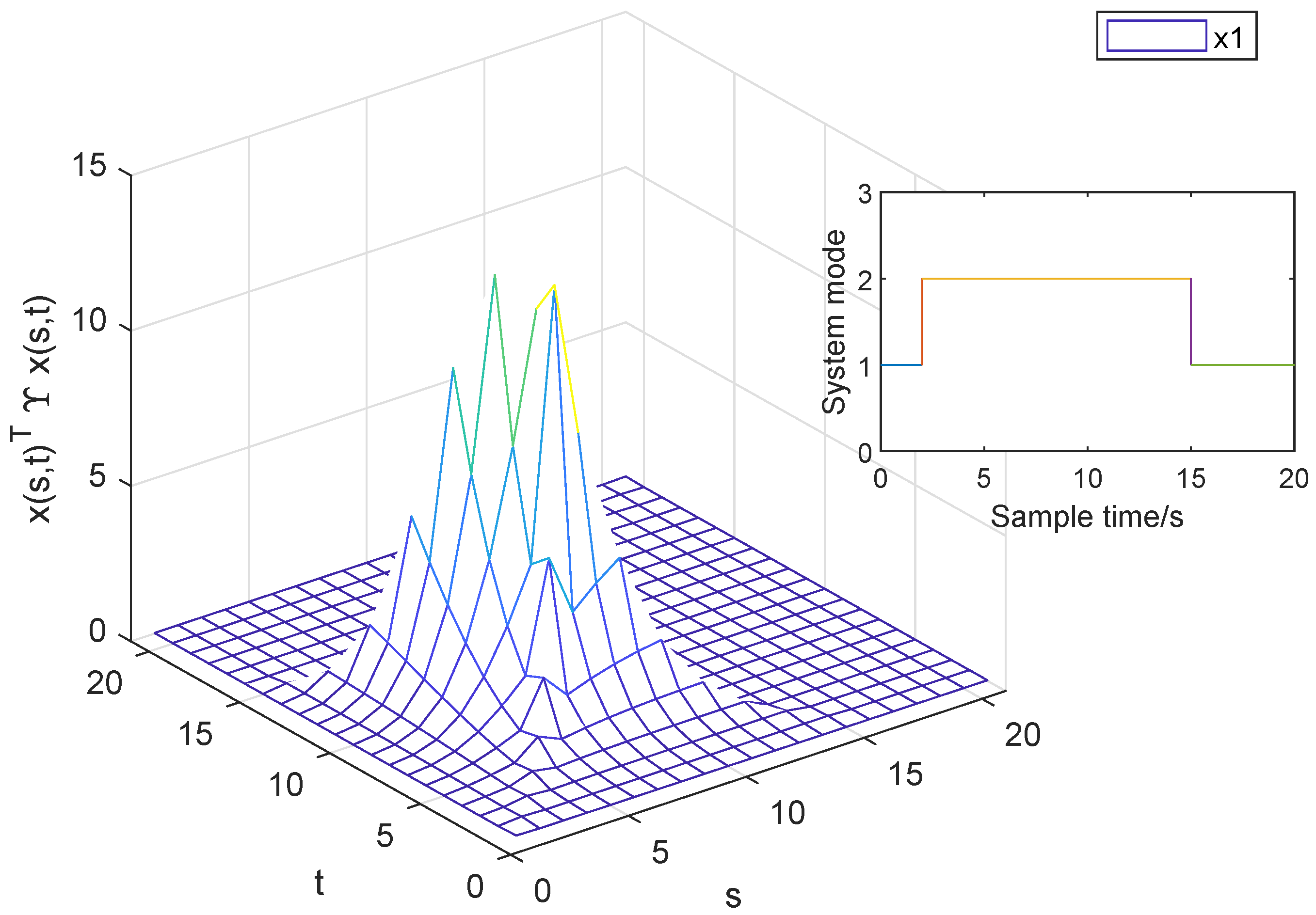
4. A Numerical Example

In this section, we demonstrate the effectiveness and advantages of the proposed method through an example.

Example 1.

Consider a 2-D switched system (1), with the corresponding parameters selected as follows:

$$A_{11}=\left[\begin{array}{cc}0.82& 0.5\\ 0.1& 0.3\end{array}\right],A_{21}=\left[\begin{array}{cc}0.1& 0.29\\ 0.5& 0.5\end{array}\right],B_{11}=\left[\begin{array}{c}0.1\\ 0.1\end{array}\right],$$

$$B_{21}=\left[\begin{array}{c}0.08\\ 0.08\end{array}\right],A_{12}=\left[\begin{array}{cc}0.5& 0.41\\ 0.5& 0.4\end{array}\right],A_{22}=\left[\begin{array}{cc}0.1& 0.4\\ 0.59& 0.2\end{array}\right],$$

$$B_{12}=\left[\begin{array}{c}0.1\\ 0.1\end{array}\right],B_{22}=\left[\begin{array}{c}0.05\\ 0.2\end{array}\right],{\rm Y}=\left[\begin{array}{cc}1& 0\\ 0& 1\end{array}\right],$$

$$c_1=0.02,N=20,N_{01}=N_{02}=1,{\varsigma }_1=1.001,$$

$${\varsigma }_2=1.002,{\beta }_1={\beta }_2=0.001,\varpi =1.$$

By calculating (34), the minimum feasible value of $c_2$ is 7.9589 when satisfying the conditions (29)–(35) of Theorem 3. By selecting $c_2=15$, a set of feasible solutions can be obtained as follows:

$$\underline{Q_{11}}=\left[\begin{array}{cc}5.6098& -1.2425\\ -1.2425& 4.6312\end{array}\right],\underline{Q_{21}}=\left[\begin{array}{cc}5.6245& -0.6523\\ -0.6523& 4.4679\end{array}\right],$$

$$\underline{Q_{12}}=\left[\begin{array}{cc}5.6076& -1.2427\\ -1.2427& 4.6288\end{array}\right],\underline{Q_{22}}=\left[\begin{array}{cc}5.6221& -0.6523\\ -0.6523& 4.4659\end{array}\right],$$

$$M_1=\left[\begin{array}{cc}-21.9486& 0\end{array}\right],M_2=\left[\begin{array}{cc}-19.0144& 0\end{array}\right],$$

$$N_1=\left[\begin{array}{cc}-0.3954& 1.1675\end{array}\right],N_2=\left[\begin{array}{cc}-0.2631& 0.7957\end{array}\right],$$

$${\sigma }_1=3.7800,{\sigma }_2=5.9200$$

From (35), by calculation, ${\tau }_{wa}^{*}=7.9222,{\alpha }_1=0.5,{\alpha }_2=0.5$. ${\alpha }_1{\tau }_{a1}+{\alpha }_2{\tau }_{a2}=0.5\times 5+0.5\times 10=7.5<{\tau }_{wa}^{*}=7.9222$. ${\alpha }_1{\tau }_{a1}+{\alpha }_2{\tau }_{a2}=0.5\times 2+0.5\times 13=7.5<{\tau }_{wa}^{*}=7.9222$. It is assumed that the boundary condition satisfies the following condition:

$$x(s,0)=\left[\begin{array}{c}0.1\\ 0.1\end{array}\right],x(0,t)=\left[\begin{array}{c}0.1\\ 0.1\end{array}\right],$$

where $0\le s\le 20$ and $0\le t\le 20$.

Furthermore, the state feedback controller is given as follows:

$$K_1=\left[\begin{array}{cc}-4.1597& -1.1160\end{array}\right],K_2=\left[\begin{array}{cc}-3.6053& -0.9679\end{array}\right],$$

$$H_1=\left[\begin{array}{cc}-0.0156& 0.2479\end{array}\right],H_2=\left[\begin{array}{cc}-0.0094& 0.1694\end{array}\right].$$

Figure 2 illustrates the state responses $x^{\top }(s,t){\rm Y}x(s,t)$ of system (1) by selecting ${\tau }_{a1}=5$ and ${\tau }_{a2}=10$. Figure 3 illustrates the state responses $x^{\top }(s,t){\rm Y}x(s,t)$ of system (1) by selecting ${\tau }_{a1}=2$ and ${\tau }_{a2}=13$. These indicate that the considered 2-D switched system (1) does not exhibit finite-region stability about $(0.02,15,20,{\rm Y},\rho (·,·\left)\right)$. Figure 4 and Figure 5 display the trajectories of $x^{\top }(s,t){\rm Y}x(s,t)$ for the resulting closed-loop system (26) when implementing the state feedback controller (23) with the specified matrices by selecting ${\tau }_{a1}=5$, ${\tau }_{a2}=10$ and ${\tau }_{a1}=2$, ${\tau }_{a2}=13$, respectively. The input saturation satisfies Equation (25). Here, we take $p=3$ as an example, and other situations are similar. The input saturations are $sat\left(u(s,t+1)\right)={\left[\begin{array}{cc}-0.0156& -1.1160\end{array}\right]}^{\top }x(s,t+1)$, $sat\left(u(s+1,t)\right)={\left[\begin{array}{cc}-0.0094& -0.9679\end{array}\right]}^{\top }x(s+1,t),$ respectively.

From Figure 4 and Figure 5, it is evident that 2-D switched system (26) exhibits the finite-region stability with respect to $(0.02,15,20,{\rm Y},\rho (·,·\left)\right)$.

5. Conclusions

This article provides sufficient conditions for the finite-region stability and stabilization for 2-D switched systems with actuator saturation. The finite region stability conditions for switched FMLSS models were obtained using the WADT method, and a control scheme was designed to achieve the finite region stability in the closed-loop system. It is worth noting that the conditions given in this article can be transformed into LMIs, which can be directly solved using the MATLAB 2023 toolbox. The last numerical example demonstrates the effectiveness of the proposed method.

References

1. Kaczorek, T. Two-Dimension Linear Systems; Spring: Berlin, Germany, 1985. [Google Scholar]
2. Du, C.; Xie, L. H Control and Filtering of Two-Dimensional Systems; Springer: Berlin, Germany, 2002. [Google Scholar]
3. Cheng, P.; Wang, H.; Stojanovic, V.; He, S.; Shi, K.; Luan, X. Asynchronous fault detection observer for 2-D Markov jump systems. IEEE Trans. Cybern. 2021, 52, 13623–13634. [Google Scholar] [CrossRef] [PubMed]
4. Yeganefar, N.; Ghamgui, M.; Moulay, E. Lyapunov theory for 2-D nonlinear Roesser models: Application to asymptotic and exponential stability. IEEE Trans. Autom. Control 2013, 58, 1299–1304. [Google Scholar] [CrossRef]
5. Duan, Z.; Liang, J.; Xiang, Z. H control for continuous-discret system in T-S fuzzy model with finite frequency specifications. Discrete Cont. Dyn.-S 2022, 15, 3155–3172. [Google Scholar]
6. Bachelier, O.; Yeganefar, N.; Mehdi, D.; Paszke, W. On stabilization of 2D Roesser Models. IEEE Trans. Autom. Control 2017, 62, 2505–2511. [Google Scholar] [CrossRef]
7. Shi, S.; Fei, Z.; Li, J. Finite-time H control of switched systems with mode-dependent average dwell time. J. Franklin Inst. 2016, 353, 221–234. [Google Scholar] [CrossRef]
8. Wang, J.; Liang, J.; Zhang, C.T. Dissipativity analysis and synthesis for positive Roesser systems under the switched mechanism and Takagi-Sugeno fuzzy rules. Inform. Sci. 2021, 546, 234–252. [Google Scholar] [CrossRef]
9. Wang, L.; Chen, W.; Li, L. Dissipative stability analysis and control of two-dimensional Fornasinia-Marchesini local state-space model. Int. J. Syst. Sci. 2017, 48, 1744–1751. [Google Scholar] [CrossRef]
10. Sakthivel, R.; Saravanakumar, T.; Kaviarasan, B.; Marshar, A.S. Dissipativity based repetitive control for switched stochastic dynamical systems. Appl. Math. Comput. 2016, 291, 340–353. [Google Scholar] [CrossRef]
11. Yang, R.; Ding, S.; Zheng, W.X. Co-design of event-triggered mechanism and dissipativity-based output feedback controller for two-dimensional systems. Automatica 2021, 130, 109694. [Google Scholar] [CrossRef]
12. Wang, J.; Liang, J.; Zhang, C.-T.; Fan, D. Robust dissipative filtering for impulsive switched positive systems described by the Fornasini-Marchesini second model. J. Franklin Inst. 2022, 359, 123–144. [Google Scholar] [CrossRef]
13. Duan, Z.; Zhou, J.; Shen, J. Finite frequency filter design for nonlinear 2-D continuous systems in T-S form. J. Franklin Inst. 2017, 354, 8606–8625. [Google Scholar] [CrossRef]
14. Duan, Z.; Ding, F.; Liang, J.; Xiang, Z. Observer-based fault detection for continuous-discrete systems in T-S fuzzy model. Nonlinear Anal. Hybrid Syst. 2023, 50, 101379. [Google Scholar] [CrossRef]
15. Li, X.; Gao, H. Robust finite frequency H filtering for uncertain 2-D Roesser systems. Automatica 2012, 48, 1163–1170. [Google Scholar] [CrossRef]
16. Ahn, C.K.; Shi, P.; Basin, M.V. Two-dimensional dissipative control and filtering for Roesser model. IEEE Trans. Autom. Control 2015, 60, 1745–1759. [Google Scholar] [CrossRef]
17. Wu, L.; Yang, R.; Shi, P.; Su, X. Stability analysis and stabilization of 2-D switched systems under arbitrary and restricted switchings. Automatica 2015, 59, 206–215. [Google Scholar] [CrossRef]
18. Xiang, Z.; Huang, S. Stability analysis and stabilization of discrete-time 2D switched systems. Circ. Syst. Signal Process. 2013, 32, 401–414. [Google Scholar] [CrossRef]
19. Duan, Z.; Xiang, Z.; Karimi, H.R. Delay-dependent exponential stabilization of positive 2D switched state-delayed systems in the Roesser model. Inform. Sci. 2014, 272, 173–184. [Google Scholar] [CrossRef]
20. Wang, J.; Liang, J. Robust finite-horizon stability and stabilization for positive switched FM-II model with actuator saturation. Nonlinear Anal. Hybrid Syst. 2020, 35, 100829. [Google Scholar] [CrossRef]
21. Fei, Z.; Shi, S.; Zhao, C.; Wu, L. Asynchronous control for 2-D switched systems with mode-dependent average dwell time. Automatica 2017, 79, 198–206. [Google Scholar] [CrossRef]
22. Yu, Q.; Lv, H. Stability analysis for discret-time switched systems with stable and unstable modes based on a weighted average dwell time approach. Nonlinear Anal. Hybrid Syst. 2020, 38, 100949. [Google Scholar] [CrossRef]
23. Zhang, T.; Cao, J.; Li, X. Lyapunov conditions for finite-time input-to-state stability of impulsive switched systems. IEEE/CAA J. Autom. Sin. 2024, 11, 1057–1059. [Google Scholar] [CrossRef]
24. Wang, W.; Qi, X.; Zhong, S.; Liu, F. Finite-time boundedness and control design of uncertain switched systems with time-varying delay under new switching rules. Int. J. Robust Nonlinear Control 2024, 34, 456–480. [Google Scholar] [CrossRef]
25. Zhang, G.; Wang, W. Finite-region stability and finite-region boundedness for 2-D Roesser models. Math. Methods Appl. Sci. 2016, 39, 5757–5769. [Google Scholar] [CrossRef]
26. Zhang, G.; Harry, H.L.; Wang, W.; Gao, J. Input-output finite-region stability and stabilization for discrete 2-D Fornasini-Marchesini models. Syst. Control Lett. 2017, 99, 9–16. [Google Scholar] [CrossRef]
27. Li, L.; Yang, R.; Feng, Z.; Wu, L. Event-triggered dissipative control for 2-D switched systems. Inf. Sci. 2022, 589, 802–812. [Google Scholar] [CrossRef]
28. Yang, R.; Li, L.; Su, X. Finite-region dissipative dynamic output feedback control for 2-D FM systems with missing measurements. Inf. Sci. 2020, 514, 1–14. [Google Scholar] [CrossRef]
29. Hua, D.; Wang, W.; Yu, W.; Wang, Y. Finite-region stabilization via dynamic output feedback for 2-D Roesser models. Math. Methods Appl. Sci. 2018, 41, 2140–2151. [Google Scholar] [CrossRef]
30. Hua, D.; Wang, W.; Ren, Y.; Yao, J. Finite-region stabilization and H control for 2-D FMLSS asynchronously switched system. J. Frankl. Inst. 2020, 357, 9127–9153. [Google Scholar] [CrossRef]
31. Yu, Q.; Zhai, G.S. New stability criteria of switched systems with unstable modes under a weighted ADT scheme. Int. J. Syst. Sci. 2021, 52, 2735–2751. [Google Scholar] [CrossRef]
32. Yu, Q.; Yuan, X.Y. Stability analysis for positive switched systems having stable and unstable subsystems based on a weighted average dwell time scheme. ISA Trans. 2023, 136, 275–283. [Google Scholar] [CrossRef]
33. Hu, T.; Lin, Z. Control Systems with Actuator Saturation; Springer: Boston, MA, USA, 2001. [Google Scholar]
Figure 1. Responses x ( s , t ) of the system with two subsystems.
Axioms 13 00752 g001
Figure 2. Responses x ( s , t ) Υ x ( s , t ) of system (1) with τ a 1 = 5 , τ a 2 = 10 and u ( s , t ) = 0 .
Axioms 13 00752 g002
Figure 3. Responses x ( s , t ) Υ x ( s , t ) of system (1) with τ a 1 = 2 , τ a 2 = 13 and u ( s , t ) = 0 .
Axioms 13 00752 g003
Figure 4. Responses x ( s , t ) Υ x ( s , t ) of system (26) with τ a 1 = 5 , τ a 2 = 10 and s a t ( u ( s , t ) ) (25).
Axioms 13 00752 g004
Figure 5. Responses x ( s , t ) Υ x ( s , t ) of system (26) with τ a 1 = 2 , τ a 2 = 13 and s a t ( u ( s , t ) ) (25).
Axioms 13 00752 g005
Disclaimer/Publisher’s Note: The statements, opinions and data contained in all publications are solely those of the individual author(s) and contributor(s) and not of MDPI and/or the editor(s). MDPI and/or the editor(s) disclaim responsibility for any injury to people or property resulting from any ideas, methods, instructions or products referred to in the content.