Bi-Starlike Function of Complex Order Involving Mathieu-Type Series in the Shell-Shaped Region

Abstract

For functions of the form $\varphi \left(\xi \right)=\xi +{\sum }_{n=2}^{\infty }{c}_n{\xi }^n$, we identified two new subclasses of bi-starlike functions and bi-convex functions by using Mathieu-type series defined in the disc $\Delta =\{\xi \in \mathbb{C}:|\xi |<1\}$. We derived constraints for $|c_2|$ and $|c_3|$, and the subclasses are connected to the shell-shaped area. The Fekete–Szegö functional properties for the aforementioned function subclasses were also investigated. Additionally, a number of related corollaries are shown.

1. Introduction

Let the collection of all functions of the construct

$$\varphi \left(\xi \right)=\xi +\sum _{n=2}^{\infty }{c}_n{\xi }^n$$

(1)

be represented by $\mathfrak{A}$, which is adjusted by the constraints ${\varphi }^{\prime }\left(0\right)=1$ and $\varphi \left(0\right)=0$ and is also analytic in the open unit disc $\Delta =\{\xi \in \mathbb{C}:|\xi |<1\}$. Also, $\mathfrak{S}$ indicates the classification of all functions in $\mathfrak{A}$ that have a univalent value in $\Delta$. The class ${\mathfrak{S}}^{*}\left(\alpha \right)$ of starlike functions of the order $\alpha$ and the class $\mathfrak{K}\left(\alpha \right)$ of convex functions of the order $\alpha$$(0\le \alpha <1)$ in $\Delta$ are two notable and thoroughly studied subclasses of $\mathfrak{S}$.

Each function $\varphi \in \mathfrak{S}$ provides an inverse ${\varphi }^{-1}$ that may be represented as

$$\begin{array}{cc}\hfill {\varphi }^{-1}\left(\varphi \left(\xi \right)\right)& =\xi (\xi \in \Delta )\hfill \\ \hfill \mathrm{and}\varphi \left({\varphi }^{-1}\left(\eta \right)\right)& =\eta \left(\right|\eta |<r_0\left(\varphi \right);r_0\left(\varphi \right)\ge 1/4)\hfill \end{array}$$

where

$${\varphi }^{-1}\left(\eta \right)=\psi \left(\eta \right)=\eta -c_2{\eta }^2+(2c_2^2-c_3){\eta }^3-(5c_2^3-5c_2{c}_3+c_4){\eta }^4+\cdots .$$

(2)

If both $\varphi$ and ${\varphi }^{-1}$ are univalent in $\Delta$, then a function $\varphi \in \mathfrak{A}$ is said to be bi-univalent in $\Delta$. In $\Delta$, let $\Sigma$ represent the class of bi-univalent functions provided by (1). The set $\Sigma$ cannot be empty, as we can see that the functions

$${\varphi }_1\left(\xi \right)={\displaystyle \frac{\xi }{1-\xi }},{\varphi }_2\left(\xi \right)={\displaystyle \frac{1}{2}}log{\displaystyle \frac{1+\xi }{1-\xi }}\mathrm{and}{\varphi }_3\left(\xi \right)=-log(1-\xi )$$

together with their respective inverses

$${\varphi }_1^{-1}\left(\eta \right)={\displaystyle \frac{\eta }{1+\eta }},{\varphi }_2^{-1}\left(\eta \right)={\displaystyle \frac{e^{2\eta }-1}{e^{2\eta }+1}}\mathrm{and}{\varphi }_3^{-1}\left(\eta \right)={\displaystyle \frac{e^{\eta }-1}{e^{\eta }}},$$

represent components of $\Sigma .$ Nevertheless, $\Sigma$ does not include the Koebe function.

Bi-starlike functions of the order $\alpha$, represented by ${\mathfrak{S}}_{\Sigma }^{*}\left(\alpha \right)$, and bi-convex functions of the order $\alpha$, represented by ${\mathfrak{K}}_{\Sigma }\left(\alpha \right)$, were previously introduced in [1] as subclasses of $\Sigma$. The researchers in [1,2] established estimates of $|a_2|$ and $|a_3|$ for functions in ${\mathfrak{S}}_{\Sigma }^{*}\left(\alpha \right)$ and ${\mathfrak{K}}_{\Sigma }\left(\alpha \right)$. Several coefficient problems were also given in [1,2,3,4,5]. Srivastava et al. [6] essentially revitalized the study of analytic and bi-univalent functions. They were followed by the studies in [1,7,8,9,10,11,12,13,14,15,16,17,18,19,20,21]. Moreover, in [22] (see also [23]), bi-prestarlike functions were investigated.

Definition 1

([24]). Consider that $\varphi \left(0\right)={\varphi }^{\prime }\left(0\right)-1=0$ is used to normalize $\varphi \in \mathfrak{A}$ in the Δ unit disc. The class of analytic functions is represented by ${\mathrm{S}}^{*}(\Phi )$, fulfilling the requirement that

$${\displaystyle \frac{z{\varphi }^{\prime }\left(\xi \right)}{\varphi \left(\xi \right)}}\prec \xi +\sqrt{1+{\xi }^2}=:\Phi \left(\xi \right),$$

In this case, $\Phi \left(0\right)=1$, the major branch of the square root, is selected.

The function $\Phi \left(\xi \right):=\xi +\sqrt{1+{\xi }^2}$ is univalent and analytic on $\Delta$, mapping $\Delta$ onto a shell-shaped region. ${\Phi }^{\prime }\left(0\right)=1=\Phi \left(0\right)$, and $\Phi \left(\xi \right)$ is a function with a positive real part. The range $\Phi (\Delta )$ is symmetric with respect to the horizontal axis. Moreover, in relation to the point $\Phi \left(0\right)=1$, it is a starlike domain (see Figure 1 and [24]) as well.

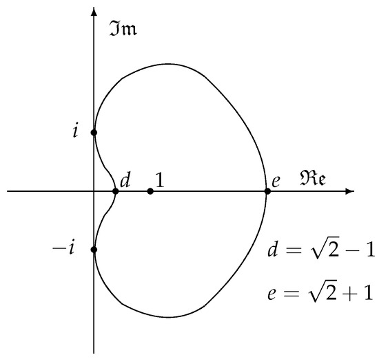
Figure 1. Boundary of $\Phi (\Delta )$.

Numerous intriguing and productive applications of a broad range of q-calculus methods; special functions; and special polynomials such as Faber, the Fibonacci, Lucas, Pell, and second-kind Chebyshev polynomials have been found in Geometric Function Theory. The elasticity of solid things was investigated by Émile Leonard Mathieu (1835–1890) in his monograph [25], which is why the following series bears his name.

$$\mathfrak{T}\left(\ell \right)=\sum _{n=1}^{\infty }{\displaystyle \frac{2n}{{\left(n^2+{\ell }^2\right)}^2}}\left(\ell >0\right).$$

(3)

The Mathieu-type series is represented by (see [26])

$$\mathfrak{T}\left(\ell ;\xi \right)=\sum _{n=1}^{\infty }{\displaystyle \frac{2n}{{\left(n^2+{\ell }^2\right)}^2}}{\xi }^n\left(\ell >0,\left|\xi \right|<1\right).$$

Bansal et al. [27] defined it for complex variables after it was first described for functions of real variables. Given that $T\left(\ell ;\xi \right)\notin \mathfrak{A}$, we can use the normalization that follows to obtain

$$\begin{array}{ccc}\hfill \mathfrak{T}\left(\ell ;\xi \right)& =& {\displaystyle \frac{{\left({\ell }^2+1\right)}^2}{2}}\sum _{n=1}^{\infty }{\displaystyle \frac{2n}{{\left(n^2+{\ell }^2\right)}^2}}{\xi }^n\hfill \end{array}$$

$$\begin{array}{ccc}& =& \xi +\sum _{n=2}^{\infty }{\displaystyle \frac{n{\left({\ell }^2+1\right)}^2}{{\left(n^2+{\ell }^2\right)}^2}}{\xi }^n,\hfill \end{array}$$

(4)

$$\begin{array}{ccc}& =& \xi +\sum _{n=2}^{\infty }{\mathfrak{G}}_n(\ell ){\xi }^n,\hfill \end{array}$$

(5)

where

$${\mathfrak{G}}_n(\ell )={\displaystyle \frac{n{\left({\ell }^2+1\right)}^2}{{\left(n^2+{\ell }^2\right)}^2}}.$$

(6)

We direct the reader to [27,28,29,30] for some similar work. We now define a novel linear operator ${\mathfrak{L}}_{\ell }:\mathfrak{A}\to \mathfrak{A}$ given by

$${\mathfrak{L}}_{\ell }\varphi \left(\xi \right):=\mathfrak{T}\left(\ell ;\xi \right)*\varphi \left(\xi \right),\xi \in \Delta ,$$

where the Hadamard product is represented by the notation “*”. Consequently, if $\varphi \in \mathfrak{A}$ has the form (1), then

$${\mathfrak{L}}_{\ell }\varphi \left(\xi \right)=\xi +\sum _{n=2}^{\infty }{\mathfrak{G}}_n(\ell )c_n{\xi }^n,\xi \in \Delta .$$

(7)

This study introduces two new subclasses of the function class $\Sigma$ of the complex order $\vartheta \in \mathbb{C}\setminus \left\{0\right\}$, including the linear operator ${\mathfrak{L}}_{\ell }$. These subclasses are inspired by the work of Silverman and Silvia [31] (see also [32]), the current study by Srivastava et al. [6], and the older work of Deniz [33] and Tang et al. [10] (see also [34,35,36,37]). In addition, we derive estimates on the coefficients $|c_2|$ and $|c_3|$ for functions in the new subclasses of the function class $\Sigma$. Additionally, other related classes are considered, and their relevance to previously established results is discussed.

Definition 2.

If the following criteria are met, a function $\varphi \left(\xi \right)\in \Sigma$ provided by (1) is considered to belong to the class ${\mathfrak{S}}_{\Sigma ,\Phi }^{\ell }(\vartheta ,\mu )$:

$$1+{\displaystyle \frac{1}{\vartheta }}\left({\displaystyle \frac{\xi {\left({\mathfrak{L}}_{\ell }\varphi \left(\xi \right)\right)}^{\prime }}{{\mathfrak{L}}_{\ell }\varphi \left(\xi \right)}}+\left({\displaystyle \frac{1+e^{i\mu }}{2}}\right){\displaystyle \frac{{\xi }^2{\left({\mathfrak{L}}_{\ell }\varphi \left(\xi \right)\right)}^{″}}{{\mathfrak{L}}_{\ell }\varphi \left(\xi \right)}}-1\right)\prec \Phi \left(\xi \right)(\mu \in (-\pi ,\pi ],\xi \in \Delta )$$

(8)

and

$$1+{\displaystyle \frac{1}{\vartheta }}\left({\displaystyle \frac{\eta {\left({\mathfrak{L}}_{\ell }\psi \left(\eta \right)\right)}^{\prime }}{{\mathfrak{L}}_{\ell }\psi \left(\eta \right)}}+\left({\displaystyle \frac{1+e^{i\mu }}{2}}\right){\displaystyle \frac{{\eta }^2{\left({\mathfrak{L}}_{\ell }\psi \left(\eta \right)\right)}^{″}}{{\mathfrak{L}}_{\ell }\psi \left(\eta \right)}}-1\right)\prec \Phi \left(\eta \right)(\mu \in (-\pi ,\pi ],\eta \in \Delta ),$$

(9)

where $\vartheta \in \mathbb{C}\setminus \left\{0\right\}$, and the function ψ is given by (2).

Definition 3.

If the following criteria are met, a function ϕ provided by (1) is considered to belong to ${\mathfrak{K}}_{\Sigma ,\Phi }^{\ell }(\vartheta ,\mu )$:

$$1+{\displaystyle \frac{1}{\vartheta }}\left({\displaystyle \frac{{[\xi {\left({\mathfrak{L}}_{\ell }\varphi \left(\xi \right)\right)}^{\prime }+\left(\frac{1+e^{i\mu }}{2}\right){\xi }^2{\left({\mathfrak{L}}_{\ell }\varphi \left(\xi \right)\right)}^{″}]}^{\prime }}{{\left({\mathfrak{L}}_{\ell }\varphi \left(\xi \right)\right)}^{\prime }}}-1\right)\prec \Phi \left(\xi \right)(\mu \in (-\pi ,\pi ],\xi \in \Delta )$$

(10)

and

$$1+{\displaystyle \frac{1}{\vartheta }}\left({\displaystyle \frac{{[\eta {\left({\mathfrak{L}}_{\ell }\psi \left(\eta \right)\right)}^{\prime }+\left(\frac{1+e^{i\mu }}{2}\right){\eta }^2{\left({\mathfrak{L}}_{\ell }\psi \left(\eta \right)\right)}^{″}]}^{\prime }}{{\left({\mathfrak{L}}_{\ell }\psi \left(\eta \right)\right)}^{\prime }}}-1\right)\prec \Phi \left(\eta \right)(\mu \in (-\pi ,\pi ],\eta \in \Delta ),$$

(11)

where $\vartheta \in \mathbb{C}\setminus \left\{0\right\}$, and ψ is represented in (2).

Remark 1.

For $\varphi \in \Sigma$ defined in (1), and for $\mu =\pi$, we note that ${\mathfrak{S}}_{\Sigma ,\Phi }^{\ell }(\vartheta ,\mu )\equiv {\mathfrak{S}}_{\Sigma ,\Phi }^{\ell }\left(\vartheta \right)$ and ${\mathfrak{K}}_{\Sigma ,\Phi }^{\ell }(\vartheta ,\mu )\equiv {\mathfrak{K}}_{\Sigma ,\Phi }^{\ell }\left(\vartheta \right)$ meet the following criteria, respectively:

$$\left[1+{\displaystyle \frac{1}{\vartheta }}\left({\displaystyle \frac{\xi {\left({\mathfrak{L}}_{\ell }\varphi \left(\xi \right)\right)}^{\prime }}{{\mathfrak{L}}_{\ell }\varphi \left(\xi \right)}}-1\right)\right]\prec \Phi \left(\xi \right)\mathrm{and}\left[1+{\displaystyle \frac{1}{\vartheta }}\left({\displaystyle \frac{\eta {\left({\mathfrak{L}}_{\ell }\psi \left(\eta \right)\right)}^{\prime }}{{\mathfrak{L}}_{\ell }\psi \left(\eta \right)}}-1\right)\right]\prec \Phi \left(\eta \right)$$

and

$$\left[1+{\displaystyle \frac{1}{\vartheta }}\left({\displaystyle \frac{\xi {\left({\mathfrak{L}}_{\ell }\varphi \left(\xi \right)\right)}^{″}}{{\left({\mathfrak{L}}_{\ell }\varphi \left(\xi \right)\right)}^{\prime }}}\right)\right]\prec \Phi \left(\xi \right)\mathrm{and}\left[1+{\displaystyle \frac{1}{\vartheta }}\left({\displaystyle \frac{\eta {\left({\mathfrak{L}}_{\ell }\psi \left(\eta \right)\right)}^{″}}{{\left({\mathfrak{L}}_{\ell }\psi \left(\eta \right)\right)}^{\prime }}}\right)\right]\prec \Phi \left(\eta \right),$$

where $\vartheta \in \mathbb{C}\setminus \left\{0\right\}\xi ,\eta \in \Delta$, and ψ is of the form (2).

Remark 2.

For $\varphi \in \Sigma$ in (1), and if $\vartheta =1,$${\mathfrak{S}}_{\Sigma ,\Phi }^{\ell }(\vartheta ,\mu )\equiv {\mathfrak{S}}_{\Sigma ,\Phi }^{\ell }\left(\mu \right)$ meets the following criteria, respectively:

$$\left({\displaystyle \frac{\xi {\left({\mathfrak{L}}_{\ell }\varphi \left(\xi \right)\right)}^{\prime }}{{\mathfrak{L}}_{\ell }\varphi \left(\xi \right)}}+\left({\displaystyle \frac{1+e^{i\mu }}{2}}\right){\displaystyle \frac{{\xi }^2{\left({\mathfrak{L}}_{\ell }\varphi \left(\xi \right)\right)}^{″}}{{\mathfrak{L}}_{\ell }\varphi \left(\xi \right)}}\right)\prec \Phi \left(\xi \right)$$

and

$$\left({\displaystyle \frac{\eta {\left({\mathfrak{L}}_{\ell }\psi \left(\eta \right)\right)}^{\prime }}{{\mathfrak{L}}_{\ell }\psi \left(\eta \right)}}+\left({\displaystyle \frac{1+e^{i\mu }}{2}}\right){\displaystyle \frac{{\eta }^2{\left({\mathfrak{L}}_{\ell }\psi \left(\eta \right)\right)}^{″}}{{\mathfrak{L}}_{\ell }\psi \left(\eta \right)}}\right)\prec \Phi \left(\eta \right).$$

Also, ${\mathfrak{K}}_{\Sigma ,\Phi }^{\ell }(\vartheta ,\mu )\equiv {\mathfrak{K}}_{\Sigma ,\Phi }^{\ell }\left(\mu \right)$ meets the following criteria:

$$\left({\displaystyle \frac{{[\xi {\left({\mathfrak{L}}_{\ell }\varphi \left(\xi \right)\right)}^{\prime }+\left(\frac{1+e^{i\mu }}{2}\right){\xi }^2{\left({\mathfrak{L}}_{\ell }\varphi \left(\xi \right)\right)}^{″}]}^{\prime }}{{\left({\mathfrak{L}}_{\ell }\varphi \left(\xi \right)\right)}^{\prime }}}\right)\prec \Phi \left(\xi \right)$$

and

$$\left({\displaystyle \frac{{[\eta {\left({\mathfrak{L}}_{\ell }\psi \left(\eta \right)\right)}^{\prime }+\left(\frac{1+e^{i\mu }}{2}\right){\eta }^2{\left({\mathfrak{L}}_{\ell }\psi \left(\eta \right)\right)}^{″}]}^{\prime }}{{\left({\mathfrak{L}}_{\ell }\psi \left(\eta \right)\right)}^{\prime }}}\right)\prec \Phi \left(\eta \right),$$

where $\mu \in (-\pi ,\pi ],\xi ,\eta \in \Delta$, and ψ is defined in (2).

2. Coefficient Estimates for the Function Classes ${\mathfrak{S}}_{\Sigma ,\Phi }^{\ell }(\mathit{\vartheta },\mathit{\mu })$ and ${\mathfrak{K}}_{\Sigma ,\Phi }^{\ell }(\mathit{\vartheta },\mathit{\mu })$

To keep things simple, let us use

$$\begin{array}{c}\hfill {\mathfrak{G}}_2(\ell )={\displaystyle \frac{2{\left({\ell }^2+1\right)}^2}{{\left(4+{\ell }^2\right)}^2}},\end{array}$$

(12)

$$\begin{array}{c}\hfill {\mathfrak{G}}_3(\ell )={\displaystyle \frac{3{\left({\ell }^2+1\right)}^2}{{\left(9+{\ell }^2\right)}^2}}\end{array}$$

(13)

where

$$\Phi \left(\xi \right):=\xi +\sqrt{1+{\xi }^2}=1+\xi +{\displaystyle \frac{1}{2}}{\xi }^2-{\displaystyle \frac{1}{8}}{\xi }^4+\cdots .$$

(14)

We require the following lemma in order to derive our main result.

Lemma 1

([38]). $|c_k|\le 2$ for each k if $h\in \mathfrak{P}$, where $\mathfrak{P}$ is the family of all functions, for which $\Re \left(h\right(\xi \left)\right)>0$, h is analytic in Δ, and

$$h\left(\xi \right)=1+c_1\xi +c_2{\xi }^2+\cdots for\xi \in \Delta .$$

The functions p and q are given by

$$p\left(\xi \right):={\displaystyle \frac{1+u\left(\xi \right)}{1-u\left(\xi \right)}}=1+p_1\xi +p_2{\xi }^2+\cdots$$

and

$$q\left(\xi \right):={\displaystyle \frac{1+v\left(\xi \right)}{1-v\left(\xi \right)}}=1+q_1\xi +q_2{\xi }^2+\cdots .$$

It follows that

$$u\left(\xi \right):={\displaystyle \frac{p\left(\xi \right)-1}{p\left(\xi \right)+1}}={\displaystyle \frac{1}{2}}\left[p_1\xi +\left(p_2-{\displaystyle \frac{p_1^2}{2}}\right){\xi }^2+\cdots \right]$$

and

$$v\left(\xi \right):={\displaystyle \frac{q\left(\xi \right)-1}{q\left(\xi \right)+1}}={\displaystyle \frac{1}{2}}\left[q_1\xi +\left(q_2-{\displaystyle \frac{q_1^2}{2}}\right){\xi }^2+\cdots \right].$$

Then $p\left(0\right)=1=q\left(0\right)$, and p and q are analytic in $\Delta$. The functions p and q have a positive real part in $\Delta ,$ and $|p_i|\le 2$ and $|q_i|\le 2$ for each i, since $u,v:\Delta \to \Delta$.

Theorem 1.

Let $\varphi \in {\mathfrak{S}}_{\Sigma ,\Phi }^{\ell }(\vartheta ,\mu )$. ϕ is defined in (1), $\vartheta \in \mathbb{C}\setminus \left\{0\right\}$, and $\mu \in (-\pi ,\pi ]$. Then,

$$|c_2|\le {\displaystyle \frac{\sqrt{2}\left|\vartheta \right|}{\sqrt{2\left|\vartheta \left[(5+3e^{i\mu }){\mathfrak{G}}_3(\ell )-(2+e^{i\mu }){\left[{\mathfrak{G}}_2(\ell )\right]}^2\right]+{(2+e^{i\mu })}^2{\left[{\mathfrak{G}}_2(\ell )\right]}^2\right|}}}$$

(15)

and

$$|c_3| \le {\displaystyle \frac{{\left|\vartheta \right|}^2}{|2+e^{i\mu }{|}^2{\left[{\mathfrak{G}}_2(\ell )\right]}^2}}+{\displaystyle \frac{\left|\vartheta \right|}{|5+3e^{i\mu }|{\mathfrak{G}}_3(\ell )}}.$$

(16)

Proof. 

According to (8) and (9),

$$1+{\displaystyle \frac{1}{\vartheta }}\left({\displaystyle \frac{\xi {\left({\mathfrak{L}}_{\ell }\varphi \left(\xi \right)\right)}^{\prime }}{{\mathfrak{L}}_{\ell }\varphi \left(\xi \right)}}+\left({\displaystyle \frac{1+e^{i\mu }}{2}}\right){\displaystyle \frac{{\xi }^2{\left({\mathfrak{L}}_{\ell }\varphi \left(\xi \right)\right)}^{″}}{{\mathfrak{L}}_{\ell }\varphi \left(\xi \right)}}-1\right)=\Phi \left(u\left(\xi \right)\right)$$

(17)

and

$$1+{\displaystyle \frac{1}{\vartheta }}\left({\displaystyle \frac{\eta {\left({\mathfrak{L}}_{\ell }\psi \left(\eta \right)\right)}^{\prime }}{{\mathfrak{L}}_{\ell }\psi \left(\eta \right)}}+\left({\displaystyle \frac{1+e^{i\mu }}{2}}\right){\displaystyle \frac{{\eta }^2{\left({\mathfrak{L}}_{\ell }\psi \left(\eta \right)\right)}^{″}}{{\mathfrak{L}}_{\ell }\psi \left(\eta \right)}}-1\right)=\Phi \left(v\left(\eta \right)\right),$$

(18)

where

$$\begin{array}{ccc}\hfill \Phi \left(u\right(\xi \left)\right)& =& \sqrt{1+{\left({\displaystyle \frac{p\left(\xi \right)-1}{p\left(\xi \right)+1}}\right)}^2}+{\displaystyle \frac{p\left(\xi \right)-1}{p\left(\xi \right)+1}}\hfill \\ & =& 1+{\displaystyle \frac{p_1}{2}}\xi +\left({\displaystyle \frac{p_2}{2}}-{\displaystyle \frac{p_1^2}{8}}\right){\xi }^2+\left({\displaystyle \frac{p_3}{2}}-{\displaystyle \frac{p_1{p}_2}{4}}\right){\xi }^3+\cdots .\hfill \end{array}$$

(19)

Likewise, we obtain

$$\Phi \left(v\left(\eta \right)\right)=1+{\displaystyle \frac{q_1}{2}}\eta +\left({\displaystyle \frac{q_2}{2}}-{\displaystyle \frac{q_1^2}{8}}\right){\eta }^2+\left({\displaystyle \frac{q_3}{2}}-{\displaystyle \frac{q_1{q}_2}{4}}\right){\eta }^3+\cdots .$$

(20)

The coefficients in (17) and (18) are now equated, giving us

$${\displaystyle \frac{1}{\vartheta }}(2+e^{i\mu })\left[{\mathfrak{G}}_2(\ell )\right]c_2={\displaystyle \frac{1}{2}}{p}_1,$$

(21)

$${\displaystyle \frac{1}{\vartheta }}\left[(5+3e^{i\mu }){\mathfrak{G}}_3(\ell )c_3-(2+e^{i\mu }){\left[{\mathfrak{G}}_2(\ell )\right]}^2{c}_2^2\right]={\displaystyle \frac{1}{2}}(p_2-{\displaystyle \frac{p_1^2}{2}})+{\displaystyle \frac{1}{8}}{p}_1^2,$$

(22)

$$-{\displaystyle \frac{1}{\vartheta }}(2+e^{i\mu })\left[{\mathfrak{G}}_2(\ell )\right]c_2={\displaystyle \frac{1}{2}}{q}_1,$$

(23)

and

$${\displaystyle \frac{1}{\vartheta }}\left([2(5+3e^{i\mu }){\mathfrak{G}}_3(\ell )-(2+e^{i\mu }){\left[{\mathfrak{G}}_2(\ell )\right]}^2]c_2^2-(5+3e^{i\mu }){\mathfrak{G}}_3(\ell )c_3\right)={\displaystyle \frac{1}{2}}(q_2-{\displaystyle \frac{q_1^2}{2}})+{\displaystyle \frac{1}{8}}{q}_1^2.$$

(24)

From (21) and (23), we have

$$p_1=-q_1$$

(25)

and

$$8{(2+e^{i\mu })}^2{\left[{\mathfrak{G}}_2(\ell )\right]}^2{c}_2^2={\vartheta }^2(p_1^2+q_1^2).$$

(26)

From (22), (24), and (26), we obtain

$$\left(2\{2\vartheta [(5+3e^{i\mu }){\mathfrak{G}}_3(\ell )-(2+e^{i\mu }){\left[{\mathfrak{G}}_2(\ell )\right]}^2]+{(2+e^{i\mu })}^2{\left[{\mathfrak{G}}_2(\ell )\right]}^2\}\right)c_2^2={\vartheta }^2(p_2+q_2).$$

(27)

Subsequently, if we apply Lemma 1 to the $p_2$ and $q_2$ coefficients, we obtain

$$|c_2| \le {\displaystyle \frac{\sqrt{2}\left|\vartheta \right|}{\sqrt{2\left|\vartheta [(5+3e^{i\mu }){\mathfrak{G}}_3(\ell )-(2+e^{i\mu }){\left[{\mathfrak{G}}_2(\ell )\right]}^2]+{(2+e^{i\mu })}^2{\left[{\mathfrak{G}}_2(\ell )\right]}^2\right|}}}.$$

After that, by deducting (22) from (24) and applying (25) to determine the bound on $|a_3|$, we obtain

$${\displaystyle \frac{2}{\vartheta }}(5+3e^{i\mu }){\mathfrak{G}}_3(\ell )(c_3-c_2^2)={\displaystyle \frac{1}{4}}(p_2-q_2).$$

When the value of $c_2^2$ is substituted from (26), we obtain

$$c_3={\displaystyle \frac{{\vartheta }^2(p_1^2+q_1^2)}{8{(2+e^{i\mu })}^2{\left[{\mathfrak{G}}_2(\ell )\right]}^2}}+{\displaystyle \frac{\vartheta (p_2-q_2)}{4(5+3e^{i\mu }){\mathfrak{G}}_3(\ell )}}.$$

When we apply Lemma 1 to the coefficients $p_1,p_2,q_1$, and $q_2$ once more, we obtain

$$|c_3| \le {\displaystyle \frac{{\left|\vartheta \right|}^2}{|2+e^{i\mu }{|}^2{\left[{\mathfrak{G}}_2(\ell )\right]}^2}}+{\displaystyle \frac{\left|\vartheta \right|}{|5+3e^{i\mu }|{\mathfrak{G}}_3(\ell )}}.$$

□

Theorem 2.

If $\varphi \in {\mathfrak{K}}_{\Sigma ,\Phi }^{\ell }(\vartheta ,\mu )$, where ϕ is defined in (1), $\vartheta \in \mathbb{C}\setminus \left\{0\right\}$, and $\mu \in (-\pi ,\pi ]$, then

$$|c_2| \le {\displaystyle \frac{\left|\vartheta \right|}{\sqrt{|\vartheta \left[3(5+3e^{i\mu }){\mathfrak{G}}_3(\ell )-4(2+e^{i\mu }){\left[{\mathfrak{G}}_2(\ell )\right]}^2\right]+2{(2+e^{i\mu })}^2{\left[{\mathfrak{G}}_2(\ell )\right]}^2|}}}$$

(28)

and

$$|c_3| \le {\displaystyle \frac{{\left|\vartheta \right|}^2}{4|2+e^{i\mu }{|}^2{\left[{\mathfrak{G}}_2(\ell )\right]}^2}}+{\displaystyle \frac{\left|\vartheta \right|}{3|5+3e^{i\mu }|{\mathfrak{G}}_3(\ell )}}.$$

(29)

Proof. 

The argument inequalities in (10) and (11) can be written similarly as follows:

$$1+{\displaystyle \frac{1}{\vartheta }}\left({\displaystyle \frac{{[\xi {\left({\mathfrak{L}}_{\ell }\varphi \left(\xi \right)\right)}^{\prime }+\left(\frac{1+e^{i\mu }}{2}\right){\xi }^2{\left({\mathfrak{L}}_{\ell }\varphi \left(\xi \right)\right)}^{″}]}^{\prime }}{{\left({\mathfrak{L}}_{\ell }\varphi \left(\xi \right)\right)}^{\prime }}}-1\right)=\Phi \left(u\left(\xi \right)\right)$$

(30)

and

$$1+{\displaystyle \frac{1}{\vartheta }}\left({\displaystyle \frac{{[\eta {\left({\mathfrak{L}}_{\ell }\psi \left(\eta \right)\right)}^{\prime }+\left(\frac{1+e^{i\mu }}{2}\right){\eta }^2{\left({\mathfrak{L}}_{\ell }\psi \left(\eta \right)\right)}^{″}]}^{\prime }}{{\left({\mathfrak{L}}_{\ell }\psi \left(\eta \right)\right)}^{\prime }}}-1\right)=\Phi \left(v\left(\eta \right)\right).$$

(31)

Following the same steps as in the proof of Theorem 1, we derive the following relations from (30) and (31).

$${\displaystyle \frac{2}{\vartheta }}(2+e^{i\mu })\left[{\mathfrak{G}}_2(\ell )\right]c_2={\displaystyle \frac{1}{2}}{p}_1,$$

(32)

$${\displaystyle \frac{1}{\vartheta }}[3(5+3e^{i\mu }){\mathfrak{G}}_3(\ell )c_3-4(2+e^{i\mu }){\left[{\mathfrak{G}}_2(\ell )\right]}^2{c}_2^2]={\displaystyle \frac{1}{2}}(p_2-{\displaystyle \frac{p_1^2}{2}})+{\displaystyle \frac{1}{8}}{p}_1^2,$$

(33)

and

$$-{\displaystyle \frac{2}{\vartheta }}(2+e^{i\mu })\left[{\mathfrak{G}}_2(\ell )\right]c_2={\displaystyle \frac{1}{2}}{q}_1,$$

(34)

$${\displaystyle \frac{1}{\vartheta }}[3(5+3e^{i\mu })(2c_2^2-c_3){\mathfrak{G}}_3(\ell )-4(2+e^{i\mu }){\left[{\mathfrak{G}}_2(\ell )\right]}^2{c}_2^2]={\displaystyle \frac{1}{2}}(q_2-{\displaystyle \frac{q_1^2}{2}})+{\displaystyle \frac{1}{8}}{q}_1^2.$$

(35)

By using (32) and (34), we arrive at

$$p_1=-q_1$$

(36)

and

$$32{(2+e^{i\mu })}^2{\left[{\mathfrak{G}}_2(\ell )\right]}^2{c}_2^2={\vartheta }^2(p_1^2+q_1^2).$$

(37)

Now, from (33), (35), and (37), we obtain

$$c_2^2={\displaystyle \frac{{\vartheta }^2(p_2+q_2)}{4[\vartheta [3(5+3e^{i\mu }){\mathfrak{G}}_3(\ell )-4(2+e^{i\mu }){\left[{\mathfrak{G}}_2(\ell )\right]}^2]+2{(2+e^{i\mu })}^2{\left[{\mathfrak{G}}_2(\ell )\right]}^2]}}.$$

(38)

Lemma 1 may be applied to the coefficients $p_2$ and $q_2$ to obtain the desired inequality, which is shown in (28).

Next, by deducting (33) from (35) and applying (36), we can determine the bound on $|a_3|$.

$${\displaystyle \frac{6}{\vartheta }}(5+3e^{i\mu })(c_3-c_2^2){\mathfrak{G}}_3(\ell )={\displaystyle \frac{1}{2}}(p_2-q_2).$$

When the value of $c_2^2$ provided by (37) is substituted, the equation above yields

$$c_3={\displaystyle \frac{\vartheta (p_2-q_2)}{12(5+3e^{i\mu }){\mathfrak{G}}_3(\ell )}}+{\displaystyle \frac{{\vartheta }^2(p_1^2+q_1^2)}{32{(2+e^{i\mu })}^2{\left[{\mathfrak{G}}_2(\ell )\right]}^2}}.$$

(39)

The required coefficient, which is given in (29), is obtained by applying Lemma 1 once again to the coefficients $p_1,p_2,q_1$, and $q_2$. □

The estimates related to the subclasses ${\mathfrak{S}}_{\Sigma ,\Phi }^{\ell }\left(\vartheta \right)$ and ${\mathfrak{K}}_{\Sigma ,\Phi }^{\ell }\left(\vartheta \right)$ specified in Remark 1 can be stated by inserting $\mu =\pi$ in Theorems 1 and 2.

Corollary 1.

If $\varphi \in {\mathfrak{S}}_{\Sigma ,\Phi }^{\ell }\left(\vartheta \right),$ then

$$|c_2|\le {\displaystyle \frac{\sqrt{2}\left|\vartheta \right|}{\sqrt{2\left|\vartheta \right|(2{\mathfrak{G}}_3(\ell )-{\left[{\mathfrak{G}}_2(\ell )\right]}^2)+{\left[{\mathfrak{G}}_2(\ell )\right]}^2}}}\mathrm{and}\left|c_3\right|\le {\displaystyle \frac{{\left|\vartheta \right|}^2}{{\left[{\mathfrak{G}}_2(\ell )\right]}^2}}+{\displaystyle \frac{\left|\vartheta \right|}{2{\mathfrak{G}}_3(\ell )}}.$$

Corollary 2.

If $\varphi \in {\mathfrak{K}}_{\Sigma ,\Phi }^{\ell }\left(\vartheta \right),$ then

$$|c_2|\le {\displaystyle \frac{\left|\vartheta \right|}{\sqrt{2\left|\vartheta \right|(3{\mathfrak{G}}_3(\ell )-2{\left[{\mathfrak{G}}_2(\ell )\right]}^2)+2{\left[{\mathfrak{G}}_2(\ell )\right]}^2}}}\mathrm{and}\left|c_3\right|\le {\displaystyle \frac{{\left|\vartheta \right|}^2}{4{\left[{\mathfrak{G}}_2(\ell )\right]}^2}}+{\displaystyle \frac{\left|\vartheta \right|}{6{\mathfrak{G}}_3(\ell )}}.$$

The coefficient estimates for the functions in the subclasses ${\mathfrak{S}}_{\Sigma ,\Phi }^{\ell }\left(\mu \right)$ and ${\mathfrak{K}}_{\Sigma ,\Phi }^{\ell }\left(\mu \right)$ specified in Remark 2 can be stated by inserting $\vartheta =1$ in Theorems 1 and 2.

Corollary 3.

If $\varphi \in {\mathfrak{S}}_{\Sigma ,\Phi }^{\ell }\left(\mu \right),$ then

$$|c_2|\le {\displaystyle \frac{\sqrt{2}}{\sqrt{2|(5+3e^{i\mu }){\mathfrak{G}}_3(\ell )-(2+e^{i\mu }){\left[{\mathfrak{G}}_2(\ell )\right]}^2|+|2+e^{i\mu }{|}^2{\left[{\mathfrak{G}}_2(\ell )\right]}^2}}}$$

and

$$|c_3|\le {\displaystyle \frac{1}{|2+e^{i\mu }{|}^2{\left[{\mathfrak{G}}_2(\ell )\right]}^2}}+{\displaystyle \frac{1}{|5+3e^{i\mu }|{\mathfrak{G}}_3(\ell )}}.$$

Corollary 4.

Let $\varphi \in {\mathfrak{K}}_{\Sigma ,\Phi }^{\ell }\left(\mu \right)$; then,

$$|c_2|\le {\displaystyle \frac{1}{\sqrt{\left\{\right[3|5+3e^{i\mu }|{\mathfrak{G}}_3(\ell )-4\left|2+e^{i\mu }\right|{\left[{\mathfrak{G}}_2(\ell )\right]}^2]+2|2+e^{i\mu }{|}^2{\left[{\mathfrak{G}}_2(\ell )\right]}^2\}}}}$$

and

$$|c_3|\le {\displaystyle \frac{1}{4{\left|2+e^{i\mu }\right|}^2{\left[{\mathfrak{G}}_2(\ell )\right]}^2}}+{\displaystyle \frac{1}{3\left|5+3e^{i\mu }\right|{\mathfrak{G}}_3(\ell )}}.$$

3. Fekete–Szegö Inequality for $\mathit{\varphi }\in {\mathfrak{S}}_{\Sigma ,\Phi }^{\ell }(\mathit{\vartheta },\mathit{\mu })$

The Fekete–Szegö functional results for the subclass ${\mathfrak{S}}_{\Sigma ,\Phi }^{\ell }(\vartheta ,\mu )$ are proven in this section. The lemmas which Zaprawa introduced in [39,40] will be used.

Lemma 2.

For ${\xi }_1,{\xi }_2\in \mathbb{C}$ and $k\in \mathbb{R}.$ If $\left|{\xi }_1\right|<R$ and $\left|{\xi }_2\right|<R,$ then 

$$\left|(k+1){\xi }_1+(k-1){\xi }_2\right|\le \left\{\begin{array}{cc}2\left|k\right|R,& \left|k\right|\ge 1,\\ 2R,& \left|k\right|\le 1.\end{array}\right.$$

Lemma 3.

For ${\xi }_1,{\xi }_2\in \mathbb{C}$ and $k,l\in \mathbb{R}.$ If $\left|{\xi }_1\right|<R$ and $\left|{\xi }_2\right|<R$, then

$$\left|(k+l){\xi }_1+(k-l){\xi }_2\right|\le \left\{\begin{array}{cc}2\left|k\right|R,& \left|k\right|\ge \left|l\right|,\\ 2\left|l\right|R,& \left|k\right|\le \left|l\right|.\end{array}\right.$$

The Fekete–Szegö functional results are given.

Theorem 3.

The classes ${\mathfrak{S}}_{\Sigma ,\Phi }^{\ell }(\vartheta ,\mu )$ and $\aleph \in \mathbb{R}$ are ϕ, as indicated by (1). Subsequently,

$$\mid c_3-\aleph c_2^2\mid \le \left\{\begin{array}{cc}{\displaystyle \frac{\left|\vartheta \right|}{3|5+3e^{i\mu }|{\mathfrak{G}}_3(\ell )}},\hfill & 0\le \mid \Phi (\aleph ,\mu )\mid \le {\displaystyle \frac{\left|\vartheta \right|}{3|5+3e^{i\mu }|{\mathfrak{G}}_3(\ell )}}\hfill \\ 2\left|\vartheta \right||\Phi (\aleph ,\mu \left)\right|,\hfill & |\Phi (\aleph ,\mu )|\ge {\displaystyle \frac{\left|\vartheta \right|}{3|5+3e^{i\mu }|{\mathfrak{G}}_3(\ell )}},\hfill \end{array}\right.$$

where

$$\Phi (\aleph ,\mu )={\displaystyle \frac{{\vartheta }^2(1-\aleph )}{4[\vartheta \left[3(5+3e^{i\mu }){\mathfrak{G}}_3(\ell )-4(2+e^{i\mu }){\left[{\mathfrak{G}}_2(\ell )\right]}^2\right]+2{(2+e^{i\mu })}^2{\left[{\mathfrak{G}}_2(\ell )\right]}^2]}}.$$

Proof. 

It may be inferred from (38) and (39) that

$$\begin{array}{ccc}\hfill c_3-\aleph c_2^2& =& {\displaystyle \frac{(1-\aleph ){\vartheta }^2(p_2+q_2)}{4[\vartheta \left[3(5+3e^{i\mu }){\mathfrak{G}}_3(\ell )-4(2+e^{i\mu }){\left[{\mathfrak{G}}_2(\ell )\right]}^2\right]+2{(2+e^{i\mu })}^2{\left[{\mathfrak{G}}_2(\ell )\right]}^2]}}+{\displaystyle \frac{\vartheta (p_2-q_2)}{12(5+3e^{i\mu }){\mathfrak{G}}_3(\ell )}}\hfill \\ & =& \left[\Phi (\aleph ,\mu )+{\displaystyle \frac{\vartheta }{12(5+3e^{i\mu }){\mathfrak{G}}_3(\ell )}}\right]p_2+\left[\Phi (\aleph ,\mu )-{\displaystyle \frac{\vartheta }{12(5+3e^{i\mu }){\mathfrak{G}}_3(\ell )}}\right]q_2,\hfill \end{array}$$

where

$$\Phi (\aleph ,\mu )={\displaystyle \frac{{\vartheta }^2(1-\aleph )}{4[\vartheta \left[3(5+3e^{i\mu }){\mathfrak{G}}_3(\ell )-4(2+e^{i\mu }){\left[{\mathfrak{G}}_2(\ell )\right]}^2\right]+2{(2+e^{i\mu })}^2{\left[{\mathfrak{G}}_2(\ell )\right]}^2]}}.$$

Applying Lemmas 1 and 3, we obtain

$$\mid c_3-\aleph c_2^2\mid \le \left\{\begin{array}{cc}{\displaystyle \frac{\left|\vartheta \right|}{3|5+3e^{i\mu }|{\mathfrak{G}}_3(\ell )}},\hfill & 0\le \mid \Phi (\aleph ,\mu )\mid \le {\displaystyle \frac{\left|\vartheta \right|}{3|5+3e^{i\mu }|{\mathfrak{G}}_3(\ell )}}\hfill \\ 2\left|\vartheta \right||\Phi (\aleph ,\mu \left)\right|,\hfill & |\Phi (\aleph ,\mu )|\ge {\displaystyle \frac{\left|\vartheta \right|}{3|5+3e^{i\mu }|{\mathfrak{G}}_3(\ell )}}.\hfill \end{array}\right.$$

Specifically, by taking $\aleph =1,$ we obtain

$$\mid c_3-c_2^2\mid \le {\displaystyle \frac{\left|\vartheta \right|}{3|5+3e^{i\mu }|{\mathfrak{G}}_3(\ell )}}.$$

□

4. Bi-Univalent Function Class ${\mathcal{G}}_{\Sigma }^{\ell }(\mathit{\vartheta },\mathit{\mu },\mathbf{\Phi })$

This section defines a subclass of bi-univalent functions that are related to shell-shaped regions and are based on Mathieu-type power series. The initial Taylor estimates $|c_2|$ and $|c_3|$ are also obtained. Additionally, for $\varphi \in {\mathcal{G}}_{\Sigma }^{\ell }(\vartheta ,\mu ,\Phi )$, we derive the Fekete–Szegö inequality.

Definition 4.

If the following criteria are met, a function $\varphi \in \Sigma$ provided by (1) is considered to belong to the class ${\mathcal{G}}_{\Sigma }^{\ell }(\vartheta ,\mu ,\Phi )$:

$$1+{\displaystyle \frac{1}{\vartheta }}\left({\displaystyle \frac{\xi {\left({\mathfrak{L}}_{\ell }\varphi \left(\xi \right)\right)}^{\prime }}{(1-\mu ){\mathfrak{L}}_{\ell }\varphi \left(\xi \right)+\mu \xi {\left({\mathfrak{L}}_{\ell }\varphi \left(\xi \right)\right)}^{\prime }}}-1\right)\prec \Phi \left(\xi \right)(\vartheta \in \mathbb{C}\setminus \left\{0\right\};0\leqq \mu <1;\xi \in \Delta )$$

(40)

and

$$1+{\displaystyle \frac{1}{\vartheta }}\left({\displaystyle \frac{\eta {\left({\mathfrak{L}}_{\ell }\psi \left(\eta \right)\right)}^{\prime }}{(1-\mu ){\mathfrak{L}}_{\ell }\psi \left(\eta \right)+\mu \xi {\left({\mathfrak{L}}_{\ell }\psi \left(\eta \right)\right)}^{\prime }}}-1\right)\prec \Phi \left(\eta \right)(\vartheta \in \mathbb{C}\setminus \left\{0\right\};0\leqq \mu <1;\eta \in \Delta ),$$

(41)

where (2) provides the function ψ.

Example 1.

A function $\varphi \in \Sigma ,$ provided by (1) for $\mu =0$ and $\vartheta \in \mathbb{C}\setminus \left\{0\right\},$ is considered to belong to the class ${\mathcal{S}}_{\Sigma }^{\ell }(\vartheta ,\Phi )$ if the following criteria are met:

$$1+{\displaystyle \frac{1}{\vartheta }}\left({\displaystyle \frac{\xi {\left({\mathfrak{L}}_{\ell }\varphi \left(\xi \right)\right)}^{\prime }}{{\mathfrak{L}}_{\ell }\varphi \left(\xi \right)}}-1\right)\prec \Phi \left(\xi \right),$$

(42)

and

$$1+{\displaystyle \frac{1}{\vartheta }}\left({\displaystyle \frac{\eta {\left({\mathfrak{L}}_{\ell }\psi \left(\eta \right)\right)}^{\prime }}{{\mathfrak{L}}_{\ell }\psi \left(\eta \right)}}-1\right)\prec \Phi \left(\eta \right),$$

(43)

for $\xi ,\eta \in \Delta$ and (2) provides the function ψ.

Theorem 4.

If $\varphi \in {\mathcal{G}}_{\Sigma }^{\ell }(\vartheta ,\mu ,\Phi )$, and ϕ is of the form (1), then

$$|c_2|\leqq {\displaystyle \frac{\left|\vartheta \right|\sqrt{2}}{\sqrt{\left|[2\vartheta ({\mu }^2-1)+{(1-\mu )}^2]{\left[{\mathfrak{G}}_2(\ell )\right]}^2+4\vartheta (1-\mu ){\mathfrak{G}}_3(\ell )\right|}}},$$

(44)

and

$$|c_3|\leqq {\displaystyle \frac{{\left|\vartheta \right|}^2}{{(1-\mu )}^2{\left[{\mathfrak{G}}_2(\ell )\right]}^2}}+{\displaystyle \frac{\left|\vartheta \right|}{2(1-\mu ){\mathfrak{G}}_3(\ell )}}.$$

(45)

$$\mid c_3-\hslash c_2^2\mid \leqq \left\{\begin{array}{cc}{\displaystyle \frac{\left|\vartheta \right|}{2(1-\mu ){\mathfrak{G}}_3(\ell )}},\hfill & 0\le \mid \phi (\hslash )\mid \le {\displaystyle \frac{\left|\vartheta \right|}{8(1-\mu ){\mathfrak{G}}_3(\ell )}}\hfill \\ 2\left|\vartheta \right|\left|\phi \right(\hslash \left)\right|,\hfill & \left|\phi (\hslash )\right|\ge {\displaystyle \frac{\left|\vartheta \right|}{8(1-\mu ){\mathfrak{G}}_3(\ell )}},\hfill \end{array}\right.$$

where

$$\phi (\hslash )={\displaystyle \frac{{\vartheta }^2(1-\hslash )}{2\left([\vartheta ({\mu }^2-1)+{(1-\mu )}^2]{\left[{\mathfrak{G}}_2(\ell )\right]}^2+4\vartheta (1-\mu ){\mathfrak{G}}_3(\ell )\right)}}.$$

Proof. 

Relations (40) and (41) imply that

$$1+{\displaystyle \frac{1}{\vartheta }}\left({\displaystyle \frac{\xi {\left({\mathfrak{L}}_{\ell }\varphi \left(\xi \right)\right)}^{\prime }}{(1-\mu ){\mathfrak{L}}_{\ell }\varphi \left(\xi \right)+\mu \xi {\left({\mathfrak{L}}_{\ell }\varphi \left(\xi \right)\right)}^{\prime }}}-1\right)=\Phi \left(u\left(\xi \right)\right)$$

(46)

and

$$1+{\displaystyle \frac{1}{\vartheta }}\left({\displaystyle \frac{\eta {\left({\mathfrak{L}}_{\ell }\psi \left(\eta \right)\right)}^{\prime }}{(1-\mu ){\mathfrak{L}}_{\ell }\psi \left(\eta \right)+\mu \xi {\left({\mathfrak{L}}_{\ell }\psi \left(\eta \right)\right)}^{\prime }}}-1\right)=\Phi \left(v\left(\eta \right)\right).$$

(47)

The coefficients in (46) and (47) are now equated, meaning that

$${\displaystyle \frac{(1-\mu )}{\vartheta }}\left[{\mathfrak{G}}_2(\ell )\right]c_2={\displaystyle \frac{1}{2}}{p}_1,$$

(48)

$${\displaystyle \frac{({\mu }^2-1)}{\vartheta }}{\left[{\mathfrak{G}}_2(\ell )\right]}^2{c}_2^2+{\displaystyle \frac{2(1-\mu )}{\vartheta }}{\mathfrak{G}}_3(\ell )c_3={\displaystyle \frac{1}{2}}(p_2-{\displaystyle \frac{p_1^2}{2}})+{\displaystyle \frac{1}{8}}{p}_1^2,$$

(49)

$$-{\displaystyle \frac{(1-\mu )}{\vartheta }}\left[{\mathfrak{G}}_2(\ell )\right]c_2={\displaystyle \frac{1}{2}}{q}_1$$

(50)

and

$${\displaystyle \frac{({\mu }^2-1)}{\vartheta }}{\left[{\mathfrak{G}}_2(\ell )\right]}^2{c}_2^2+{\displaystyle \frac{2(1-\mu )}{\vartheta }}{\mathfrak{G}}_3(\ell )(2c_2^2-c_3)={\displaystyle \frac{1}{2}}(q_2-{\displaystyle \frac{q_1^2}{2}})+{\displaystyle \frac{1}{8}}{q}_1^2.$$

(51)

According to (48) and (50),

$$c_2={\displaystyle \frac{\vartheta p_1}{2(1-\mu )\left[{\mathfrak{G}}_2(\ell )\right]}}={\displaystyle \frac{-\vartheta q_1}{2(1-\mu )\left[{\mathfrak{G}}_2(\ell )\right]}},$$

(52)

which gives

$$p_1=-q_1$$

(53)

and

$$8{(1-\mu )}^2{\left[{\mathfrak{G}}_2(\ell )\right]}^2{c}_2^2={\vartheta }^2(p_1^2+q_1^2).$$

(54)

Using (52) and (53), we obtain (49) plus (51), and we have

$$2\left([2\vartheta ({\mu }^2-1)+{(1-\mu )}^2]{\left[{\mathfrak{G}}_2(\ell )\right]}^2+4\vartheta (1-\mu ){\mathfrak{G}}_3(\ell )\right)c_2^2={\vartheta }^2(p_2+q_2).$$

(55)

Thus,

$$c_2^2={\displaystyle \frac{{\vartheta }^2(p_2+q_2)}{2\left([\vartheta ({\mu }^2-1)+{(1-\mu )}^2]{\left[{\mathfrak{G}}_2(\ell )\right]}^2+4\vartheta (1-\mu ){\mathfrak{G}}_3(\ell )\right)}}.$$

(56)

When Lemma 1 is applied to the coefficients $p_2$ and $q_2,$ we instantly obtain

$$|c_2{|}^2\leqq {\displaystyle \frac{{2\left|\vartheta \right|}^2}{\left|[2\vartheta ({\mu }^2-1)+{(1-\mu )}^2]{\left[{\mathfrak{G}}_2(\ell )\right]}^2+4\vartheta (1-\mu ){\mathfrak{G}}_3(\ell )\right|}}.$$

(57)

The desired estimate on $|c_2|$ supplied in (44) is provided by the last inequality.

Then, by deducting (51) from (49), we can determine the bound on $|c_3|$.

$$\begin{array}{ccc}\hfill {\displaystyle \frac{4(1-\mu )}{\vartheta }}{\mathfrak{G}}_3(\ell )c_3-{\displaystyle \frac{4(1-\mu )}{\vartheta }}{\mathfrak{G}}_3(\ell )c_2^2& =& {\displaystyle \frac{1}{2}}(p_2-q_2)+{\displaystyle \frac{1}{8}}(p_1^2-q_1^2)\hfill \\ \hfill c_3& =& c_2^2+{\displaystyle \frac{\vartheta (p_2-q_2)}{8(1-\mu ){\mathfrak{G}}_3(\ell )}}.\hfill \end{array}$$

(58)

Applying (52), (53), and (58),

$$\begin{array}{ccc}\hfill c_3& =& {\displaystyle \frac{{\vartheta }^2(p_1^2+q_1^2)}{8{(1-\mu )}^2{\left[{\mathfrak{G}}_2(\ell )\right]}^2}}+{\displaystyle \frac{\vartheta (p_2-q_2)}{8(1-\mu ){\mathfrak{G}}_3(\ell )}}.\hfill \end{array}$$

(59)

Lemma 1 is easily applied once again for the coefficients $p_2$ and $q_2,$.

$$|c_3|\leqq {\displaystyle \frac{{\left|\vartheta \right|}^2}{{(1-\mu )}^2{\left[{\mathfrak{G}}_2(\ell )\right]}^2}}+{\displaystyle \frac{\left|\vartheta \right|}{2(1-\mu ){\mathfrak{G}}_3(\ell )}}.$$

It may be inferred from (56) and (59) that

$$\begin{array}{ccc}\hfill c_3-\hslash c_2^2& =& {\displaystyle \frac{(1-\hslash ){\vartheta }^2(p_2+q_2)}{2\left([\vartheta ({\mu }^2-1)+{(1-\mu )}^2]{\left[{\mathfrak{G}}_2(\ell )\right]}^2+4\vartheta (1-\mu ){\mathfrak{G}}_3(\ell )\right)}}+{\displaystyle \frac{\vartheta (p_2-q_2)}{8(1-\mu ){\mathfrak{G}}_3(\ell )}}\hfill \\ & =& \left[\phi (\hslash )+{\displaystyle \frac{\vartheta }{8(1-\mu ){\mathfrak{G}}_3(\ell )}}\right]p_2+\left[\phi (\hslash )-{\displaystyle \frac{\vartheta }{8(1-\mu ){\mathfrak{G}}_3(\ell )}}\right]q_2\hfill \end{array}$$

where

$$\phi (\hslash )={\displaystyle \frac{{\vartheta }^2(1-\hslash )}{2\left([\vartheta ({\mu }^2-1)+{(1-\mu )}^2]{\left[{\mathfrak{G}}_2(\ell )\right]}^2+4\vartheta (1-\mu ){\mathfrak{G}}_3(\ell )\right)}}.$$

Consequently, using Lemma 1, we obtain

$$\mid c_3-\hslash c_2^2\mid \le \left\{\begin{array}{cc}{\displaystyle \frac{\left|\vartheta \right|}{2(1-\mu ){\mathfrak{G}}_3(\ell )}},\hfill & 0\le \mid \phi (\hslash )\mid \le {\displaystyle \frac{\left|\vartheta \right|}{8(1-\mu ){\mathfrak{G}}_3(\ell )}}\hfill \\ 2\left|\vartheta \right|\left|\phi \right(\hslash \left)\right|,\hfill & \left|\phi (\hslash )\right|\ge {\displaystyle \frac{\left|\vartheta \right|}{8(1-\mu ){\mathfrak{G}}_3(\ell )}}.\hfill \end{array}\right.$$

Specifically, by assuming $\hslash =1,$ we obtain

$$\mid c_3-c_2^2\mid \le {\displaystyle \frac{\left|\vartheta \right|}{2(1-\mu ){\mathfrak{G}}_3(\ell )}}.$$

This concludes the proof of Theorem 4. □

5. Conclusions

We discovered the initial coefficients of functions in the classes connected to shell-shaped regions and proposed two new subclasses of bi-starlike and bi-convex functions of a complex order involving Mathieu-type series in the open unit disc. The Fekete–Szegö inequalities for function in these classes were also found. As corollaries, several of these results have novel significance. Additionally, we found that by fixing specific functions, such as functions associated with Bell numbers and shell-like curves associated with Fibonacci numbers, several subclasses of starlike functions have recently become known (see [29,41,42]). Furthermore, one can find new conclusions for the subclasses discussed in this paper by using functions associated with conic domains and rational functions in place of $\Phi$ in (14).

References

- Brannan, D.A.; Taha, T.S. On some classes of bi-univalent functions. Studia Univ. Babeś-Bolyai Math. 1986, 31, 70–77. [Google Scholar]
- Taha, T.S. Topics in Univalent Function Theory. Ph.D. Thesis, University of London, London, UK, 1981. [Google Scholar]
- Brannan, D.A.; Clunie, J.G. Aspects of Contemporary Complex Analysis. In Proceedings of the NATO Advanced Study Institute, University of Durham, Durham, UK, 1–20 July 1979; Academic Press: New York, NY, USA; London, UK, 1980. [Google Scholar]
- Lewin, M. On a coefficient problem for bi-univalent functions. Proc. Am. Math. Soc. 1967, 18, 63–68. [Google Scholar] [CrossRef]
- Netanyahu, E. The minimal distance of the image boundary from the origin and the second coefficient of a univalent function in |z|< 1. Arch. Rational Mech. Anal. 1969, 32, 100–112. [Google Scholar]
- Srivastava, H.M.; Raducanu, D.; Zaprawa, P.A. Certain subclass of analytic functions defined by means of differential subordination. Filomat 2016, 30, 3743–3757. [Google Scholar] [CrossRef]
- El-Qadeem, A.H.; Mamon, M.A. Estimation of initial Maclaurin coefficients of certain subclasses of bounded bi-univalent functions. J. Egypt. Math. Soc. 2019, 27, 16. [Google Scholar] [CrossRef]
- El-Qadeem, A.H.; Saleh, S.A.; Mamon, M.A. Bi-univalent functions classes defined by using a second Einstein function. J. Function Spaces 2022, 2022, 6933153. [Google Scholar] [CrossRef]
- Frasin, B.A.; Aouf, M.K. New subclasses of bi-univalent functions. Appl. Math. Lett. 2011, 24, 1569–1573. [Google Scholar] [CrossRef]
- Tang, H.; Deng, G.-T.; Li, S.-H. Coefficient estimates for new subclasses of Ma-Minda bi-univalent functions. J. Ineq. Appl. 2013, 2013, 317. [Google Scholar] [CrossRef]
- Li, X.-F.; Wang, A.-P. Two new subclasses of bi-univalent functions. Int. Math. Forum 2012, 7, 1495–1504. [Google Scholar]
- Saleh, S.A.; El-Qadeem, A.H.; Mamon, M.A. Faber polynomial coefficient estimation of subclass of bi-subordinate univalent functions. Turkish J. Ineq. 2019, 3, 23–33. [Google Scholar]
- Saleh, S.A.; El-Qadeem, A.H.; Mamon, M.A. Some estimation about Tayler-Maclaurin coefficients of generalized subclasses of bi-univalent functions. Tbilisi Math. J. 2020, 13, 23–32. [Google Scholar] [CrossRef]
- Srivastava, H.M.; Mishra, A.K.; Gochhayat, P. Certain subclasses of analytic and bi-univalent functions. Appl. Math. Lett. 2010, 23, 1188–1192. [Google Scholar] [CrossRef]
- Srivastava, H.M.; Murugusundaramoorthy, G.; Magesh, N. Certain subclasses of bi-univalent functions associated with the Hohlov operator. Glob. J. Math. Anal. 2013, 1, 67–73. [Google Scholar]
- Srivastava, H.M.; Altınkaya, S.; Yalçin, S. Certain subclasses of bi-univalent functions associated with the Horadam polynomials. Iran. J. Sci. Technol. Trans. A Sci. 2019, 43, 1873–1879. [Google Scholar] [CrossRef]
- Srivastava, H.M.; Kamali, M.; Urdaletova, A. A study of the Fekete-Szegö functional and coefficient estimates for subclasses of analytic functions satisfying a certain subordination condition and associated with the Gegenbauer polynomials. AIMS Math. 2022, 7, 2568–2584. [Google Scholar] [CrossRef]
- Srivastava, H.M.; Wanas, A.K.; Srivastava, R. Applications of the q-Srivastava-Attiya operator involving a certain family of bi-univalent functions associated with the Horadam polynomials. Symmetry 2021, 13, 1230. [Google Scholar] [CrossRef]
- Srivastava, H.M.; Wanas, A.K.; Murugusundaramoorthy, G. A certain family of bi-univalent functions associated with the Pascal distribution series based upon the Horadam polynomials. Surv. Math. Appl. 2021, 16, 193–205. [Google Scholar]
- Srivastava, H.M. Operators of basic (or q-) calculus and fractional q-calculus and their applications in geometric function theory of complex analysis. Iran. J. Sci. Technol. Trans. A Sci. 2020, 44, 327–344. [Google Scholar] [CrossRef]
- Srivastava, H.M.; Motamednezhad, A.; Adegani, E.A. Faber polynomial coefficient estimates for bi-univalent functions defined by using differential subordination and a certain fractional derivative operator. Mathematics 2020, 8, 172. [Google Scholar] [CrossRef]
- Jahangiri, J.M.; Hamidi, S.G. Advances on the coefficients of bi-prestarlike functions. Comptes Rendus Acad. Sci. Paris 2016, 354, 980–985. [Google Scholar] [CrossRef]
- Murugusundaramoorthy, G.; Güney, H.Ö.; Vijaya, K. Coefficient bounds for certain suclasses of bi-prestarlike functions associated with the Gegenbauer polynomial. Adv. Stud. Contemp. Math. 2022, 32, 5–15. [Google Scholar]
- Raina, R.K.; Sokól, J. On Coefficient estimates for a certain class of starlike functions. Hacettepe J. Math. Statist. 2015, 44, 1427–1433. [Google Scholar] [CrossRef]
- Mathieu, E.L. Traité de Physique Mathematique. VI–VII: Theory del Elasticité des Corps solides (PART 2); Gauthier-Villars: Paris, France, 1890. [Google Scholar]
- Tomovski, Z. New integral and series representations of the generalized Mathieu series. Appl. Anal. Discrete Math. 2008, 2, 205–212. [Google Scholar] [CrossRef]
- Bansal, D.; Sokól, J. Geometric properties of Mathieu–type power series inside unit disk. J. Math. Ineq. 2019, 13, 911–918. [Google Scholar] [CrossRef]
- Bansal, D.; Sokól, J. Univalency of starlikeness of Harwitz-Lerch Zeta function inside unit disk. J. Math. Ineq. 2017, 11, 863–871. [Google Scholar] [CrossRef]
- Dziok, J.; Raina, R.K.; Sokół, J. On certain subclasses of starlike functions related to a shell-like curve connected with Fibonacci numbers. Math. Comput. Model. 2013, 57, 1203–1211. [Google Scholar] [CrossRef]
- Nunokawa, M.; Sokól, J. On an extension of Sakaguchi’s result. J. Math. Ineq. 2015, 9, 683–697. [Google Scholar] [CrossRef]
- Silverman, H.; Silvia, E.M. Characterizations for subclasses of univalent functions. Math. Japon. 1999, 50, 103–109. [Google Scholar]
- Silverman, H. A class of bounded starlike functions. Int. J. Math. Math. Sci. 1994, 17, 249–252. [Google Scholar] [CrossRef]
- Deniz, E. Certain subclasses of bi-univalent functions satisfying subordinate conditions. J. Class. Anal. 2013, 2, 49–60. [Google Scholar] [CrossRef]
- Deniz, E.; Jahangiri, J.M.; Hamidi, S.G.; Kına, S.K. Faber polynomial coefficients for generalized bi-subordinate functions of complex order. J. Math. Ineq. 2018, 12, 645–653. [Google Scholar] [CrossRef]
- Çağlar, M.; Deniz, E. Initial coefficients for a subclass of bi-univalent functions defined by Salagean differential operator. Commun. Fac. Sci. Univ. Ank. Ser. A1 Math. Stat. 2017, 66, 85–91. [Google Scholar]
- Deniz, E.; Kamali, M.; Korkmaz, S. A certain subclass of bi-univalent functions associated with Bell numbers and q-Srivastava Attiya operator. AIMS Math. 2020, 5, 7259–7271. [Google Scholar] [CrossRef]
- Çağlar, M.; Palpandy, G.; Deniz, E. Unpredictability of initial coefficient bounds for m-fold symmetric bi-univalent starlike and convex functions defined by subordinations. Afr. Mat. 2018, 29, 793–802. [Google Scholar] [CrossRef]
- Pommerenke, C. Univalent Functions; Vandenhoeck & Ruprecht: Göttingen, Germany, 1975. [Google Scholar]
- Zaprawa, P. On the Fekete-Szegö problem for classes of bi-univalent functions. Bull. Belg. Math. Soc. Simon Stevin 2014, 21, 1–192. [Google Scholar] [CrossRef]
- Zaprawa, P. Estimates of initial coefficients for Biunivalent functions. Abstr. Appl. Anal. 2014, 2014, 357480. [Google Scholar] [CrossRef]
- Cho, N.E.; Kumar, S.; Kumar, V.; Ravichandran, V.; Serivasatava, H.M. Starlike functions related to the Bell numbers. Symmetry 2019, 11, 219. [Google Scholar] [CrossRef]
- Kanas, S.; Răducanu, D. Some classes of analytic functions related to conic domains. Math. Slovaca 2014, 64, 1183–1196. [Google Scholar] [CrossRef]
Disclaimer/Publisher’s Note: The statements, opinions and data contained in all publications are solely those of the individual author(s) and contributor(s) and not of MDPI and/or the editor(s). MDPI and/or the editor(s) disclaim responsibility for any injury to people or property resulting from any ideas, methods, instructions or products referred to in the content. |
© 2024 by the authors. Licensee MDPI, Basel, Switzerland. This article is an open access article distributed under the terms and conditions of the Creative Commons Attribution (CC BY) license (https://creativecommons.org/licenses/by/4.0/).