Refined Iterative Method for a Common Variational Inclusion and Common Fixed-Point Problem with Practical Applications

Abstract

This paper introduces a novel parallel method for solving common variational inclusion and common fixed-point (CVI-CFP) problems. The proposed algorithm provides a strong convergence theorem established under specific conditions associated with the CVI-CFP problem. Numerical simulations demonstrate the algorithm’s efficacy in the context of signal recovery problems involving various types of blurred filters. The results highlight the algorithm’s potential for practical applications in image processing and other fields.

1. Introduction

Throughout this paper, let $\mathbb{N},\mathbb{R}$, and ${\mathbb{R}}^{+}$ be the set of all positive integers, the set of real numbers and the set of positive real numbers, respectively. We also denote ${\mathbb{R}}_0^{+}={\mathbb{R}}^{+}\cup \left\{0\right\}.$ Let $H:=\left(H,⟨·,·⟩\right)$ be a Hilbert space with the induced norm $\parallel ·\parallel .$ For $M\in \mathbb{N}$, we denote $\left[M\right]:=\{1,2,\cdots ,M\}$. The following classes of mappings are often used in this article:

$$\mathfrak{X}=\left\{X_i:H\to H,i\in \left[M\right]\right\}\mathrm{and}\mathfrak{Y}=\left\{Y_i:H\to 2^H,i\in \left[M\right]\right\}.$$

The problem to find $v\in H$, such that

$$0\in (X_i+Y_i)v$$

(1)

for all $X_i\in \mathfrak{X}$ and $Y_i\in \mathfrak{Y}$, is known as the common variational inclusion problem, also known as CVIP. In particular, when $M=1,$ the CVIP (1) is simply the variational inclusion problem, and in this case, its solution set is denoted by ${(X_1+Y_1)}^{-1}\left(0\right).$ Here, the set of all solutions of (1) is given by $\mathrm{CVIP}(\mathfrak{X},\mathfrak{Y})$. In other words,

$${\displaystyle \mathrm{CVIP}(\mathfrak{X},\mathfrak{Y})=\bigcap _{i\in \left[M\right]}{\left(X_i+Y_i\right)}^{-1}\left(0\right).}$$

(2)

These types of problems have been applied to real-world approaches, including signal recovery and image recovery problems, which require finding solutions satisfying a number of constraints formulated using nonlinear functional models [1,2]. Interestingly, we can effectively exploit these problems by combining them with the concept of fixed-point theory. For a map $Z:H\to H$, the set of all fixed points of Z is the set $\mathrm{Fix}\left(Z\right):=\left\{u\in H:Zu=u\right\}.$ Let $\mathcal{Z}$ be a collection of mappings $Z_i:H\to H$ for all $i\in \left[M\right].$ We define the set of all common fixed points of all $Z_i\in \mathcal{Z}$ as

$$\mathrm{CFix}\left(\mathcal{Z}\right)=\{x\in X:x\in \mathrm{Fix}\left(Z_i\right)\mathrm{for}\mathrm{all}{Z}_i\in \mathcal{Z}\}.$$

Recently, the problem to find $v\in H$, such that

$$v\in \mathrm{CVIP}(\mathfrak{X},\mathfrak{Y})\cap \mathrm{CFix}\left(\mathcal{Z}\right)$$

(3)

was introduced. It is called a common variational inclusion and common fixed-point problem (CVI-CFP problem), see [3]. As CVI-CFP problems encompass both (common) variational inclusion and (common) fixed-point problems as special cases, this allows for a more comprehensive approach to solving a wider range of problems.

Over the past decades, various algorithms have been developed to solve such problems. These include the forward–backward splitting method [4,5] and the inertial proximal algorithm [6]. Tseng then proposed the forward–backward–forward method, also known as Tseng’s method, in [7]. For recent advancements, refer to [8,9,10,11,12,13]. Recently, a parallel algorithm was developed to determine a common fixed point for G-nonexpansive maps in H, and to solve signal recovery problems in a situation that the noise type is unknown in [1]. A parallel algorithm based on the inertial Mann iteration was presented in [3] to establish a weak convergence for solving (3) in H. For other results related to the problem (3), see [14,15,16,17,18,19]. Moreover, Antón-Sancho [20] investigated fixed points of automorphisms in the moduli space of vector bundles over compact Riemann surfaces, highlighting their effects on the space’s structure and symmetries.

The aforementioned problems have been recognized as valuable tools in mathematical models, including variational inequality problems and split feasibility problems. These models are applied in many areas, such as signal and image processing, economics, engineering, and especially machine learning (see [21,22,23,24,25], for example). In particular, a generalized time iteration (GTI) method, introduced in [26], effectively solves dynamic optimization problems with occasionally binding constraints, significantly advancing macroeconomic, financial, and labor economics modeling (see also the references cited herein). In recent years, environmental concerns, particularly PM2.5 pollution, have become pressing issues. In [27], the authors employed machine learning algorithms to estimate ground-level PM2.5 concentrations using micro-satellite image processing. Machine learning has emerged as a powerful tool for PM2.5 prediction due to its ability to analyze vast datasets and utilize complex algorithms, see [28,29,30]. It can effectively address the PM2.5 problem, which can help to improve air quality management.

In this article, we present an algorithm to address problem (3). In Section 3, we provide a strong convergence result for the proposed method. Finally, Section 4 presents the application of our proposed algorithms to the signal recovery problem under various blurred filters.

2. Preliminaries

In this section, we introduce essential notations, definitions, and preliminary results that will be utilized in the subsequent sections. Here, ⇀ and → denote weak convergence and strong convergence, respectively.

Proposition 1.

For $u,v\in H$,

$$\begin{array}{cc}\hfill {\parallel u+v\parallel }^2& ={\parallel u\parallel }^2+2⟨u,v⟩+{\parallel v\parallel }^2;\hfill \end{array}$$

(4)

$$\begin{array}{cc}\hfill {\parallel u+y\parallel }^2& \le {\parallel u\parallel }^2+2⟨v,u+v⟩.\hfill \end{array}$$

(5)

Proposition 2.

Let ${\alpha }_0\in \mathbb{R}$, and let ${\alpha }_1,{\alpha }_2,{\alpha }_3\in [0,1]$, such that ${\alpha }_1+{\alpha }_2+{\alpha }_3=1$. Then, for any $u,v,w\in H$,

$$\begin{array}{cc}\hfill \parallel {\alpha }_{0}u+(1-{\alpha }_0){v\parallel }^2& ={\alpha }_0{\parallel u\parallel }^2+(1-{\alpha }_0){\parallel v\parallel }^2-{\alpha }_0(1-{\alpha }_0){\parallel u-v\parallel }^2;\hfill \end{array}$$

(6)

$$\begin{array}{ll}\hfill \parallel {\alpha }_{1}u+{\alpha }_{2}v+{\alpha }_3{w\parallel }^2& ={\alpha }_1{\parallel u\parallel }^2+{\alpha }_2{\parallel v\parallel }^2+{\alpha }_3{\parallel w\parallel }^2\hfill \\ & -{\alpha }_1{\alpha }_2{\parallel u-v\parallel }^2-{\alpha }_1{\alpha }_3{\parallel u-w\parallel }^2-{\alpha }_2{\alpha }_3{\parallel v-w\parallel }^2.\end{array}$$

(7)

Lemma 1

([31]). Let $\left\{a_k\right\}$ and $\left\{c_k\right\}$ be sequences in ${\mathbb{R}}_0^{+}$, such that ${\displaystyle \sum _{k=1}^{\infty }{c}_k<\infty }$, and let $\left\{b_k\right\}$ be a sequence in $\mathbb{R}$, such that ${\displaystyle \underset{k\to \infty }{lim\; sup}{b}_k\le 0}$. Suppose that for any $k\in \mathbb{N}$, $a_{k+1}\le (1-{\gamma }_k)a_k+{\gamma }_k{b}_k+c_k,$ where $\left\{{\gamma }_k\right\}$ is a sequence in $(0,1)$ with ${\displaystyle \sum _{k=1}^{\infty }{\gamma }_k=\infty .}$ Then, the sequence $a_k$ converges to zero.

Lemma 2

([32]). Let $\left\{{\Gamma }_k\right\}$ be a sequence in ${\mathbb{R}}_0^{+}$, such that there exists a subsequence $\left\{{\Gamma }_{k_q}\right\}$ with ${\Gamma }_{k_q}<{\Gamma }_{k_q+1}$ for all $q\in \mathbb{N}$. Then, the following hold.

(i)

The sequence ${\{\Omega \left(k\right)\}}_{k\ge k^{*}}$ given by

$$\begin{array}{c}\hfill \Omega \left(k\right):=max\{n\le k:{\Gamma }_n<{\Gamma }_{n+1}\}\end{array}$$

(8)

is nondecreasing and ${\displaystyle \underset{k\to \infty }{lim}\Omega \left(k\right)=\infty .}$

(ii)

For all $k\ge k^{*}$, ${\Gamma }_{\Omega \left(k\right)}\le {\Gamma }_{\Omega \left(k\right)+1}$ and ${\Gamma }_k\le {\Gamma }_{\Omega \left(k\right)+1}.$

Definition 1.

A mapping $Z:H\to H$ is called L-Lipschitz (or Lipschitz when there is no ambiguity) if $L\ge 0$ exists satisfying

$$\parallel Zu-Zv\parallel \le L\parallel u-v\parallel \mathit{for}\mathit{all}u,v\in X.$$

It is called L-contractive when $L\in [0,1),$ and nonexpansive when $L=1.$

Let C be a nonempty, closed, and convex subset of H. For $x\in H$, define $P_C:H\to C$ by $P_{C}x:=\arg {min}_{y\in C}\parallel x-y\parallel .$ The inequality

$$\begin{array}{c}\hfill ⟨x-P_{C}x,y-P_{C}x⟩\le 0\end{array}$$

(9)

has been known to distinguish the metric projection $P_C$ for any $x\in H$ and $y\in C$.

Next, we recall some background and notation from fixed-point theory in the context of our setting.

Definition 2.

Let $Z:H\to H$ be a map with $\mathrm{Fix}\left(Z\right)\ne \varnothing .$ Then,

(i)

[33] Z is μ-demicontractive if there exists $\mu \in [0,1)$, such that for all $x\in H$ and for all $p\in \mathrm{Fix}\left(Z\right)$,

$${\parallel Zx-p\parallel }^2\le {\parallel x-p\parallel }^2+\mu {\parallel x-Zx\parallel }^2.$$

(ii)

[34] Z is demiclosed at zero if for any $\left\{v_k\right\}\in H$, $v_k\rightharpoonup v\mathit{and}Z{v}_k\to 0\mathit{imply}Zv=0.$

Definition 3

([35]). Let $Y:H\to 2^H$ be a map. Then, Y is called monotone if for any pair $\left((x,u),(y,v)\right)$ in the graph of Y (denoted by $\mathrm{G}\left(Y\right)),$ $⟨u-v,x-y⟩\ge 0.$ Moreover, it is called maximal if its graph is not a proper subgraph of the graph of another monotone map.

Equivalently, Y is maximally monotone if and only if for each $(x,u)\in H\times H$, $(x,u)\in \mathrm{G}\left(Y\right)$ whenever $⟨u-v,x-y⟩\ge 0$ for all $(y,v)\in \mathrm{G}\left(Y\right).$

Lemma 3

([36]). Let $X:H\to H$ be a mapping, and let $Y:H\to 2^H$ be a maximally monotone mapping. If $A_{\gamma }:={\left(I+\gamma Y\right)}^{-1}\left(I-\gamma X\right)$ and $\gamma >0$, then $\mathrm{Fix}\left(A_{\gamma }\right)={(X+Y)}^{-1}\left(0\right)$.

Lemma 4

([37]). Let $X:H\to H$ be a Lipschitz and monotone mapping, and let $Y:H\to 2^H$ be a maximally monotone mapping. Then, $X+Y$ is maximally monotone.

Lemma 5

([38]). Suppose that $Z:H\to H$ is a μ-demicontractive mapping with $\mathrm{Fix}\left(Z\right)\ne \varnothing$. Let $Z_{\alpha }=\alpha I+(1-\alpha )Z$ where $\alpha \in (\mu ,1)$. Then

(i)

$\parallel Z_{\alpha }{x-p\parallel }^2\le {\parallel x-p\parallel }^2-(1-\alpha )(\alpha -\mu ){\parallel Zx-x\parallel }^2$ for all $x\in H$ and all $p\in \mathrm{Fix}\left(Z\right)$;

(ii)

$\mathrm{Fix}\left(Z\right)$ is closed and convex.

3. Main Result

We first list all conditions required for our purposed algorithm below.

(C1) 

Each $X_i\in \mathfrak{X}$ is $i_L$-Lipschitz and monotone, and each $Y_i\in \mathfrak{Y}$ is maximally monotone.

(C2) 

$\left\{p_k^i\right\}$ is a sequence in ${\mathbb{R}}_0^{+}$ such that ${\displaystyle \sum _{k=1}^{\infty }{p}_k^i<\infty }$ and $\left\{q_k^i\right\}\subset [1,\infty )$.

(C3) 

Each $Z_i\in \mathcal{Z}$ is ${\mu }_i$-demicontractive, and the map $\varphi :H\to \mathbb{R}$ is differentiable.

(C4) 

$\Omega :=\mathrm{CVIP}(\mathfrak{X},\mathfrak{Y})\cap \mathrm{CFix}\left(\mathcal{Z}\right)$ is nonempty.

(C5) 

$\left\{{\xi }_k\right\}$ is a sequence in ${\mathbb{R}}_0^{+}$, $\left\{{\theta }_k\right\},\left\{{\eta }_k\right\}\subset (0,1)$ and $\left\{{\alpha }_k^i\right\}\subset ({\mu }_i,{\overline{\alpha }}_i)\subset (0,1)$ for some ${\overline{\alpha }}_i\in {\mathbb{R}}^{+}$.

(C6) 

$I-Z_i$ is demiclosed at zero and ${\displaystyle \underset{k\to \infty }{lim}{q}_k^i=1}$ for all $i\in \left[M\right]$.

(C7) 

$0<{\eta }^{*}\le {\eta }_k\le \overline{\eta }<1-{\theta }_k$ for some ${\eta }^{*},\overline{\eta }\in {\mathbb{R}}^{+}$, ${\displaystyle \underset{k\to \infty }{lim}{\theta }_k=\underset{k\to \infty }{lim}\frac{{\xi }_k}{{\theta }_k}\parallel v_k-v_{k-1}\parallel =0}$, ${\displaystyle \sum _{k=1}^{\infty }{\theta }_k=\infty }$ and $\Psi :=\nabla \varphi$ is $\phi$-contractive.

We now proceed to present our algorithm, namely Algorithm 1.

Lemma 6.

Assume that conditions (C1) and (C2) are satisfied. Then, Algorithm 1 generates a sequence $\left\{{\delta }_k^i\right\}$ converging to ${\delta }_i$ within the range $\left[min\left\{{\delta }_1^i,{\displaystyle \frac{{\lambda }_i}{{\mathcal{L}}_i}}\right\},{\delta }_1^i+p_i\right]$ where ${\displaystyle p_i=\sum _{k=1}^{\infty }{p}_k^i}$.

Proof. 

We first note that $X_i{\phi }_k\ne X_i{r}_k^i$ since $X_i$ is $L_i$-Lipschitz for all $i\in \left[M\right].$ Then,

$$\begin{array}{c}\hfill {\displaystyle \frac{{\lambda }_i{q}_k^i\parallel {\phi }_k-r_k^i\parallel }{\parallel X_i{\phi }_k-X_i{r}_k^i\parallel }}\ge {\displaystyle \frac{{\lambda }_i{q}_k^i\parallel {\phi }_k-r_k^i\parallel }{L_i\parallel {\phi }_k-r_k^i\parallel }}={\displaystyle \frac{{\lambda }_i{q}_k^i}{L_i}}\ge {\displaystyle \frac{{\lambda }_i}{L_i}}.\end{array}$$

Following the method outlined in the proof of Lemma 3.1 in [39], we can conclude that

$${\displaystyle \underset{k\to \infty }{lim}{\delta }_k^i={\delta }_i\in \left[min\left\{{\delta }_1^i,\frac{{\lambda }_i}{L_i}\right\},{\delta }_1^i+p_i\right].}$$

   □

Remark 1.

By the proof of Lemma 6, the mapping $X_i$ must satisfy the Lipschitz condition, which is a necessary condition for establishing the strong convergence of Algorithm 1, as demonstrated in Theorem 1.

Lemma 7.

Assume that conditions (C1) and (C2) are satisfied. If ${\phi }_k=r_k^i=Z_i{s}_k^i$ for all $i\in \left[M\right]$ in Algorithm 1, then ${\phi }_k\in \Omega .$

Proof. 

The Lipschitz condition of $X_i$ and ${\phi }_k=r_k^i$ implies that for all $i\in \left[M\right]$,

$$\begin{array}{c}\hfill \parallel r_k^i-s_k^i\parallel \le {\delta }_k^i{L}_i\parallel {\phi }_k-r_k^i\parallel =0.\end{array}$$

This means that $r_k^i=s_k^i$ for all $i\in \left[M\right]$. Hence, ${\phi }_k=r_k^i=s_k^i=Z_i{s}_k^i$ for all $i\in \left[M\right]$ and so ${\phi }_k\in \mathrm{CFix}\left(\mathcal{Z}\right)$. From ${\phi }_k=r_k^i$, we obtain that, for all $i\in \left[M\right]$,

$$\begin{array}{c}\hfill {\phi }_k={\left(I+{\delta }_k^i{Y}_i\right)}^{-1}(I-{\delta }_k^i{X}_i){\phi }_k.\end{array}$$

By Lemma 3, ${\phi }_k\in \mathrm{CVIP}(\mathfrak{X},\mathfrak{Y})$. Therefore, ${\phi }_k\in \Omega$.    □

Algorithm 1 Modified parallel algorithm.

1: Let $v_0,v_1\in H$, ${\lambda }_i\in (0,1)$ and ${\delta }_1^i\in {\mathbb{R}}^{+}$ for all $i\in \left[M\right]$, and set $k:=1.$ 2: Iterative Steps: Construct the sequence $\left\{v_k\right\}$ through the following iterative procedure: Step 1. Set ${\phi }_k=v_k+{\xi }_k(v_k-v_{k-1})$ and calculate, for all $i\in \left[M\right]$, $$\begin{array}{c}\hfill r_k^i={\left(I+{\delta }_k^i{Y}_i\right)}^{-1}(I-{\delta }_k^i{X}_i){\phi }_k.\end{array}$$ Step 2. Calculate, for all $i\in \left[M\right]$, $$\begin{array}{c}\hfill s_k^i=r_k^i-{\delta }_k^i(X_i{r}_k^i-X_i{\phi }_k)\mathrm{and}{u}_k^i=Z_i{s}_k^i-{\alpha }_k^i(Z_i{s}_k^i-s_k^i).\end{array}$$ If ${\phi }_k=r_k^i=Z_i{s}_k^i$ for all $i\in \left[M\right]$, then stop and ${\phi }_k\in \Omega$. Otherwise, go to Step 3. Step 3. Evaluate $$\begin{array}{c}\hfill {\tilde{u}}_k=argmax\left\{\parallel u_k^i-{\phi }_k\parallel :i\in \left[M\right]\right\}\mathrm{and}{v}_{k+1}={\theta }_k\Psi \left(v_k\right)+(1-{\theta }_k-{\eta }_k)v_k+{\eta }_k{\tilde{u}}_k.\end{array}$$ Step 4. Update, for all $i\in \left[M\right]$, $${\delta }_{k+1}^i=\left\{\begin{array}{ll}min\left\{{\displaystyle \frac{{\lambda }_i{q}_k^i\parallel {\phi }_k-r_k^i\parallel }{\parallel X_i{\phi }_k-X_i{r}_k^i\parallel }},{\delta }_k^i+p_k^i\right\}& \mathrm{if}{X}_i{\phi }_k\ne X_i{r}_k^i;\\ {\delta }_k^i+p_k^i& \mathrm{otherwise}.\end{array}\right.$$ Replace k by $k+1$ and go back to Step 1.

Lemma 8.

Assume that conditions (C1)–(C5) are satisfied. If $v\in \Omega$, then for each $i\in \left[M\right]$,

$$\begin{array}{c}\hfill \parallel u_k^i{-v\parallel }^2+(1-{\alpha }_k^i)({\alpha }_k^i-{\mu }_i)\parallel Z_i{s}_k^i-s_k^i{\parallel }^2+\left[1-{\left({\varpi }_k^i\right)}^2\right]\parallel {\phi }_k-r_k^i{\parallel }^2\le {\parallel {\phi }_k-v\parallel }^2\end{array}$$

(10)

and

$$\begin{array}{c}\hfill \parallel s_k^i-{\phi }_k\parallel \le \left(1+{\varpi }_k^i\right)\parallel {\phi }_k-r_k^i\parallel \end{array}$$

(11)

where ${\varpi }_k^i={\lambda }_i{q}_k^i{\displaystyle \frac{{\delta }_k^i}{{\delta }_{k+1}^i}}$.

Proof. 

Let $i\in \left[M\right].$ From the definitions of $s_k^i$ and ${\delta }_k^i$, we obtain that

$$\begin{array}{c}\hfill \parallel s_k^i-r_k^i\parallel ={\delta }_k^i\parallel X_i{r}_k^i-X_i{\phi }_k\parallel \le {\varpi }_k^i\parallel r_k^i-{\phi }_k\parallel .\end{array}$$

(12)

By (4) and (12) with the conditions of ${\delta }_k^i$ and $X_i$,

$$\begin{array}{cc}\hfill \parallel s_k^i{-v\parallel }^2& =\parallel r_k^i{-v\parallel }^2-2{\delta }_k^i⟨r_k^i-v,X_i{r}_k^i-X_i{\phi }_k⟩+{\left({\delta }_k^i\right)}^2{\parallel X_i{r}_k^i-X_i{\phi }_k\parallel }^2\hfill \\ \hfill & \le \parallel r_k^i-{\phi }_k{\parallel }^2-2⟨r_k^i-{\phi }_k,r_k^i-{\phi }_k⟩+2⟨r_k^i-{\phi }_k,r_k^i-v⟩+{\parallel {\phi }_k-v\parallel }^2\hfill \\ \hfill & -2{\delta }_k^i⟨r_k^i-v,X_i{r}_k^i-X_i{\phi }_k⟩+{\left({\varpi }_k^i\right)}^2{\parallel r_k^i-{\phi }_k\parallel }^2\hfill \\ \hfill & =\parallel {\phi }_k{-v\parallel }^2-\left[1-{\left({\varpi }_k^i\right)}^2\right]{\parallel {\phi }_k-r_k^i\parallel }^2\hfill & \\ & -2⟨r_k^i-v,{\phi }_k-r_k^i-{\delta }_k^i(X_i{\phi }_k-X_i{r}_k^i)⟩.\hfill \end{array}$$

(13)

By the property of $r_k^i$, we have that

$$\begin{array}{c}\hfill (I-{\delta }_k^i{X}_i){\phi }_k\in (I+{\delta }_k^i{Y}_i)r_k^i.\end{array}$$

This implies that there is $g_k^i\in Y_i{r}_k^i$ such that

$$\begin{array}{c}\hfill g_k^i={\displaystyle \frac{1}{{\delta }_k^i}}\left({\phi }_k-r_k^i-{\delta }_k^i{X}_i{\phi }_k\right).\end{array}$$

Since $X_i+Y_i$ is maximally monotone,

$$\begin{array}{c}\hfill ⟨X_i{r}_k^i+g_k^i,r_k^i-v⟩\ge 0.\end{array}$$

Consequently,

$$\begin{array}{c}\hfill ⟨r_k^i-v,{\phi }_k-r_k^i-{\delta }_k^i(X_i{\phi }_k-X_i{r}_k^i)⟩\ge 0.\end{array}$$

Then, by (13),

$$\begin{array}{c}\hfill \parallel s_k^i{-v\parallel }^2\le \parallel {\phi }_k{-v\parallel }^2-\left[1-{\left({\varpi }_k^i\right)}^2\right]{\parallel {\phi }_k-r_k^i\parallel }^2.\end{array}$$

From Lemma 5 $\left(i\right)$, we have that for all $i\in \left[M\right]$,

$$\begin{array}{cc}\hfill \parallel u_k^i{-v\parallel }^2& \le \parallel s_k^i{-v\parallel }^2-(1-{\alpha }_k^i)({\alpha }_k^i-{\mu }_i){\parallel Z_i{s}_k^i-s_k^i\parallel }^2\hfill \\ \hfill & \le \parallel {\phi }_k{-v\parallel }^2-\left[1-{\left({\varpi }_k^i\right)}^2\right]\parallel {\phi }_k-r_k^i{\parallel }^2-(1-{\alpha }_k^i)({\alpha }_k^i-{\mu }_i){\parallel Z_i{s}_k^i-s_k^i\parallel }^2.\hfill \end{array}$$

Finally, by the triangle inequality and (12), we obtain the inequality (11). □

Lemma 9.

Assume that conditions (C1)–(C5) are satisfied. If there exists a subsequence $\left\{{\phi }_{k_m}\right\}$ of $\left\{{\phi }_k\right\}$, such that ${\phi }_{k_m}\rightharpoonup \overline{r}\in H$ and ${\displaystyle \underset{m\to \infty }{lim}\parallel {\phi }_{k_m}-r_{k_m}^i\parallel =\underset{m\to \infty }{lim}\parallel Z_i{s}_{k_m}^i-s_{k_m}^i\parallel =0}$ for all $i\in \left[M\right]$, then $\overline{r}\in \Omega$.

Proof. 

As ${\displaystyle \underset{k\to \infty }{lim}{q}_k^i=1}$ and ${\displaystyle \underset{k\to \infty }{lim}{\delta }_k^i={\delta }_i}$, we have that ${\displaystyle \underset{k\to \infty }{lim}{\varpi }_k^i={\lambda }_i>0.}$ From (11) and ${\displaystyle \underset{m\to \infty }{lim}\parallel {\phi }_{k_m}-r_{k_m}^i\parallel =0}$,

$${\displaystyle \underset{m\to \infty }{lim}\parallel {\phi }_{k_m}-s_{k_m}^i\parallel =0.}$$

Then, $s_{k_m}^i\rightharpoonup \overline{r}$ for all $i\in \left[M\right]$. It follows from ${\displaystyle \underset{m\to \infty }{lim}\parallel Z_i{s}_{k_m}^i-s_{k_m}^i\parallel =0}$ and (C6) that $\overline{r}\in \mathrm{CFix}\left(\mathcal{Z}\right)$.

Next, we show that ${\displaystyle \overline{r}\in \bigcap _{i\in \left[M\right]}{\left(X_i+Y_i\right)}^{-1}\left(0\right)}$. Let $(v_i,u_i)\in G\left(X_i+Y_i\right)$ for all $i\in \left[M\right]$. Thus $u_i-X_i{v}_i\in Y_i{v}_i$ for all $i\in \left[M\right]$. By the definition of $r_k^i$,

$${\displaystyle \frac{1}{{\delta }_{k_m}^i}}\left({\phi }_{k_m}-r_{k_m}^i-{\delta }_{k_m}^i{X}_i{\phi }_{k_m}\right)\in Y_i{r}_{k_m}^i$$

for all $i\in \left[M\right]$. By the condition of $Y_i$, for all $i\in \left[M\right]$,

$$\begin{array}{c}\hfill ⟨v_i-r_{k_m}^i,u_i-X_i{v}_i-{\displaystyle \frac{1}{{\delta }_{k_m}^i}}\left({\phi }_{k_m}-r_{k_m}^i-{\delta }_{k_m}^i{X}_i{\phi }_{k_m}\right)⟩\ge 0.\end{array}$$

Thus, for each $i\in \left[M\right]$,

$$\begin{array}{cc}\hfill ⟨v_i-r_{k_m}^i,u_i⟩& \ge ⟨v_i-r_{k_m}^i,X_i{v}_i+{\displaystyle \frac{1}{{\delta }_{k_m}^i}}\left({\phi }_{k_m}-r_{k_m}^i-{\delta }_{k_m}^i{X}_i{\phi }_{k_m}\right)⟩\hfill \\ \hfill & =⟨v_i-r_{k_m}^i,X_i{v}_i-X_i{r}_{k_m}^i⟩+⟨v_i-r_{k_m}^i,X_i{r}_{k_m}^i-X_i{\phi }_{k_m}⟩\hfill \\ \hfill & +{\displaystyle \frac{1}{{\delta }_{k_m}^i}}⟨v_i-r_{k_m}^i,{\phi }_{k_m}-r_{k_m}^i⟩\hfill \\ \hfill & \ge ⟨v_i-r_{k_m}^i,X_i{r}_{k_m}^i-X_i{\phi }_{k_m}⟩+{\displaystyle \frac{1}{{\delta }_{k_m}^i}}⟨v_i-r_{k_m}^i,{\phi }_{k_m}-r_{k_m}^i⟩.\hfill \end{array}$$

By the Lipschitz continuity of $X_i$, ${\displaystyle \underset{m\to \infty }{lim}\parallel {\phi }_{k_m}-r_{k_m}^i\parallel =0,}$ and By Lemma 6, we have that ${\displaystyle ⟨v_i-\overline{r},u_i⟩=\underset{m\to \infty }{lim}⟨v_i-r_{k_m}^i,u_i⟩\ge 0}$ for all $i\in \left[M\right].$ By the maximal monotonicity of $X_i+Y_i$, we obtain that $0\in \left(X_i+Y_i\right)\overline{r}$ for all $i\in \left[M\right]$ which means that ${\displaystyle \overline{r}\in \bigcap _{i\in \left[M\right]}{\left(X_i+Y_i\right)}^{-1}\left(0\right)}$ and thus $\overline{r}\in \Omega$. □

Lemma 10.

If $Y:H\to 2^H$ is maximally monotone and $X:H\to H$ is Lipschitz and monotone, then the set ${(X+Y)}^{-1}\left(0\right)$ is closed and convex.

Proof. 

Firstly, let $\left\{v_k\right\}$ be a sequence in ${(X+Y)}^{-1}\left(0\right)$ converging to v. Then, $0\in (X+Y)\left(v_k\right)$. By Lemma 4, we obtain that the mapping $X+Y$ is maximally monotone, and so

$$\begin{array}{c}\hfill ⟨u,x-v_k⟩\ge 0\end{array}$$

for all $(x,u)\in \mathrm{G}\left(Y\right)$. This follows that

$$\begin{array}{c}\hfill ⟨u,x-v⟩=\underset{k\to \infty }{lim}⟨u,x-v_k⟩\ge 0\end{array}$$

for all $(x,u)\in \mathrm{G}\left(Y\right)$. Similarly, by the maximal monotonicity of $X+Y$, $0\in \left(X+Y\right)\left(v\right)$ which means that $v\in {(X+Y)}^{-1}\left(0\right)$. Therefore, ${(X+Y)}^{-1}\left(0\right)$ is closed. Finally, let $c,d\in {(X+Y)}^{-1}\left(0\right)$ and $t\in [0,1]$. Then, $0\in (X+Y)\left(c\right)\cap (X+Y)\left(d\right)$. We subsequently have that

$$\begin{array}{c}\hfill ⟨-u,c-x⟩\ge 0\mathrm{and}⟨-u,d-x⟩\ge 0\end{array}$$

for all $(x,u)\in \mathrm{G}\left(Y\right)$. Thus

$$\begin{array}{c}\hfill ⟨-u,tc+(1-t)d-x⟩=t⟨-u,c-x⟩+(1-t)⟨-u,d-x⟩\ge 0\end{array}$$

for all $(x,u)\in \mathrm{G}\left(Y\right)$. It follows that $tc+(1-t)d\in {(X+Y)}^{-1}\left(0\right)$. Therefore, the set ${(X+Y)}^{-1}\left(0\right)$ is convex. □

Now, we are ready to present our strong convergence result.

Theorem 1.

Assume that conditions (C1)–(C7) are satisfied. Then, the sequence $\left\{v_k\right\}$, which is generated by Algorithm 1, strongly converges to $\upsilon :=\left(P_{\Omega }\circ \Psi \right)\upsilon$.

Proof. 

Let $p\in \Omega$. As ${\displaystyle \underset{k\to \infty }{lim}\left[1-{\left({\varpi }_k^i\right)}^2\right]=1-{\lambda }_i^2>0,}$ there exists $m_i\in \mathbb{N}$, such that $1-{\left({\varpi }_k^i\right)}^2>0$ for all $i\in \left[M\right]$ and all $k\ge k_0$, where ${\displaystyle k_0=\underset{i\in \left[M\right]}{max}{m}_i}$. By (10), (C5), the definition of ${\phi }_k$ and ${\displaystyle \underset{k\to \infty }{lim}\frac{{\xi }_k}{{\theta }_k}\parallel v_k-v_{k-1}\parallel =0}$, we have that, for all $i\in \left[M\right]$ and all $k\ge k_0$,

$$\begin{array}{c}\hfill \parallel u_k^i-p\parallel \le \parallel {\phi }_k-p\parallel \le \parallel v_k-p\parallel +{\xi }_k\parallel v_k-v_{k-1}\parallel \le \parallel v_k-p\parallel +{\theta }_k{R}_1\end{array}$$

for some $R_1>0$. Thus,

$$\begin{array}{c}\hfill \parallel {\tilde{u}}_k-p\parallel \le \parallel {\phi }_k-p\parallel \le \parallel v_k-p\parallel +{\xi }_k\parallel v_k-v_{k-1}\parallel \le \parallel v_k-p\parallel +{\theta }_k{R}_1\end{array}$$

(14)

for all $k\ge k_0$.

Next, set $c_k:={\eta }_k{\tilde{u}}_k+(1-{\eta }_k)v_k$, ${\gamma }_k:={\theta }_k(1-\phi )$ and $R_2:={\displaystyle \frac{\parallel \Psi \left(p\right)-p\parallel +R_1}{1-\phi }}$ for all $k\in \mathbb{N}$. Then

$$\begin{array}{c}\hfill \parallel c_k-v_k\parallel ={\eta }_k\parallel {\tilde{u}}_k-v_k\parallel \le \parallel {\tilde{u}}_k-v_k\parallel .\end{array}$$

(15)

It follows from (14) that

$$\begin{array}{cc}\hfill \parallel c_k-p\parallel & \le {\eta }_k\parallel {\tilde{u}}_k-p\parallel +(1-{\eta }_k)\parallel v_k-p\parallel \hfill \\ \hfill & \le {\eta }_k\parallel v_k-p\parallel +{\eta }_k{\xi }_k\parallel v_k-v_{k-1}\parallel +(1-{\eta }_k)\parallel v_k-p\parallel \hfill \\ \hfill & \le \parallel v_k-p\parallel +{\xi }_k\parallel v_k-v_{k-1}\parallel \hfill \end{array}$$

(16)

for all $k\ge k_0$. By the $\phi$-contractivity of $\Psi$ and (14), we have the following calculation:

$$\begin{array}{cc}\hfill \parallel v_{k+1}-p\parallel & =\parallel {\theta }_k\Psi \left(v_k\right)+(1-{\theta }_k-{\eta }_k)v_k+{\eta }_k{\tilde{u}}_k-p\parallel \hfill \\ \hfill & \le {\theta }_k\parallel \Psi \left(v_k\right)-p\parallel +(1-{\theta }_k-{\eta }_k)\parallel v_k-p\parallel +{\eta }_k\parallel {\tilde{u}}_k-p\parallel \hfill \\ \hfill & \le {\theta }_k\parallel \Psi \left(v_k\right)-\Psi \left(p\right)\parallel +{\theta }_k\parallel \Psi \left(p\right)-p\parallel +(1-{\theta }_k)\parallel v_k-p\parallel +{\eta }_k{\theta }_k{R}_1\hfill \\ \hfill & \le {\theta }_k\phi \parallel v_k-p\parallel +(1-{\theta }_k)\parallel v_k-p\parallel +{\theta }_k\parallel \Psi \left(p\right)-p\parallel +{\theta }_k{R}_1\hfill \\ \hfill & \le (1-{\gamma }_k)\parallel v_k-p\parallel +{\theta }_k\left(\parallel \Psi \left(p\right)-p\parallel +R_1\right)\hfill \\ \hfill & =(1-{\gamma }_k)\parallel v_k-p\parallel +{\gamma }_k{R}_2\hfill \\ \hfill & \le max\left\{\parallel v_k-p\parallel ,R_2\right\}\hfill \end{array}$$

for all $k\ge k_0$. Thus, $\parallel v_{k+1}-p\parallel \le max\left\{\parallel v_{k_0}-p\parallel ,R_2\right\}$ for all $k\ge k_0$. Consequently, the sequences $\left\{v_k\right\}$ and $\{\Psi \left(v_k\right)\}$ are bounded. It implies by Lemma 5 $\left(ii\right)$ and Lemma 10 that there is a unique $\upsilon \in \Omega$, such that $\upsilon =\left(P_{\Omega }\circ \Psi \right)\upsilon$. It follows from (9) that for any $y\in \Omega$,

$$\begin{array}{c}\hfill ⟨\Psi \left(\upsilon \right)-\upsilon ,y-\upsilon ⟩\le 0.\end{array}$$

(17)

Now, for each $k\in \mathbb{N}$, set

$${{\rm Y}}_k:={\parallel v_k-\upsilon \parallel }^2.$$

Applying (14), we obtain that for all $k\ge k_0$,

$$\begin{array}{cc}\hfill \parallel {\tilde{u}}_k{-\upsilon \parallel }^2\le {\parallel {\phi }_k-\upsilon \parallel }^2& \le {\left(\parallel v_k-\upsilon \parallel +{\theta }_k{R}_1\right)}^2\hfill \\ \hfill & ={{\rm Y}}_k+{\theta }_k\left(2R_1\parallel v_k-\upsilon \parallel +{\theta }_k{R}_1^2\right)\hfill \\ \hfill & \le {{\rm Y}}_k+{\theta }_k{R}_3\hfill \end{array}$$

(18)

for some $R_3>0$. Let ${\displaystyle R_4=\underset{k\in \mathbb{N}}{sup}\left\{\parallel v_k-\upsilon \parallel ,{\xi }_k\parallel v_k-v_{k-1}\parallel \right\}}$. By using the same technique as (16), we have that, for all $k\ge k_0$,

$$\begin{array}{cc}\hfill \parallel c_k{-\upsilon \parallel }^2& \le {{\rm Y}}_k+3R_4{\xi }_k\parallel v_k-v_{k-1}\parallel .\hfill \end{array}$$

(19)

From the property of $\Psi$, (5), (6), (15), and (19), we have the following:

$$\begin{array}{cc}\hfill {{\rm Y}}_{k+1}& =\parallel (1-{\theta }_k)(c_k-\upsilon )+{\theta }_k\left(\Psi \left(v_k\right)-\Psi \left(\upsilon \right)\right)-{\theta }_k(v_k-c_k)-{\theta }_k{(\upsilon -\Psi \left(\upsilon \right)\parallel }^2\hfill \\ \hfill & \le \parallel (1-{\theta }_k)(c_k-\upsilon )+{\theta }_k\left(\Psi \left(v_k\right)-\Psi \left(\upsilon \right)\right){\parallel }^2\hfill & \\ & -2{\theta }_k⟨v_k-c_k+\upsilon -\Psi \left(\upsilon \right),v_{k+1}-\upsilon ⟩\hfill \\ \hfill & \le (1-{\theta }_k)\parallel c_k{-\upsilon \parallel }^2+{\theta }_k{\parallel \Psi \left(v_k\right)-\Psi \left(\upsilon \right)\parallel }^2+2{\theta }_k⟨c_k-v_k,v_{k+1}-\upsilon ⟩\hfill & \\ & +2{\theta }_k⟨\Psi \left(\upsilon \right)-\upsilon ,v_{k+1}-\upsilon ⟩\hfill \\ \hfill & \le (1-{\theta }_k)\left({{\rm Y}}_k+3R_4{\xi }_k\parallel v_k-v_{k-1}\parallel \right)+{\theta }_k{\phi }^2{{\rm Y}}_k\hfill & \\ & +2{\theta }_k\parallel c_k-v_k\parallel \parallel v_{k+1}-\upsilon \parallel +2{\theta }_k⟨\Psi \left(\upsilon \right)-\upsilon ,v_{k+1}-\upsilon ⟩\hfill \\ \hfill & \le (1-{\theta }_k){{\rm Y}}_k+3R_4{\xi }_k\parallel v_k-v_{k-1}\parallel +{\theta }_k\phi {{\rm Y}}_k+2R_4{\theta }_k\parallel {\tilde{u}}_k-v_k\parallel \hfill & \\ & +2{\theta }_k⟨\Psi \left(\upsilon \right)-\upsilon ,v_{k+1}-\upsilon ⟩\hfill \\ \hfill & =(1-{\gamma }_k){{\rm Y}}_k+{\gamma }_k\left[{\displaystyle \frac{3R_4}{1-\phi }}·{\displaystyle \frac{{\xi }_k}{{\theta }_k}}\parallel v_k-v_{k-1}\parallel +{\displaystyle \frac{2R_4}{1-\phi }}\parallel {\tilde{u}}_k-v_k\parallel \right]\hfill & \\ & +{\displaystyle \frac{2{\gamma }_k}{1-\phi }}⟨\Psi \left(\upsilon \right)-\upsilon ,v_{k+1}-\upsilon ⟩.\hfill \end{array}$$

(20)

Then, from (7) and (18), we obtain that for all $k\ge k_0$,

$$\begin{array}{ccc}\hfill {{\rm Y}}_{k+1}& \le {\theta }_k\parallel \Psi \left(v_k\right){-\upsilon \parallel }^2+(1-{\theta }_k-{\eta }_k){{\rm Y}}_k+{\eta }_k{\parallel {\tilde{u}}_k-\upsilon \parallel }^2\hfill & \\ & -{\eta }_k(1-{\theta }_k-{\eta }_k){\parallel v_k-{\tilde{u}}_k\parallel }^2\hfill \\ \hfill & \le {\theta }_k\parallel \Psi \left(v_k\right){-\upsilon \parallel }^2+(1-{\theta }_k){{\rm Y}}_k+{\eta }_k{\theta }_k{R}_3-{\eta }_k(1-{\theta }_k-{\eta }_k){\parallel v_k-{\tilde{u}}_k\parallel }^2\hfill \\ \hfill & \le {{\rm Y}}_k+{\theta }_k\left(\parallel \Psi \left(v_k\right){-\upsilon \parallel }^2+R_3\right)-{\eta }_k(1-{\theta }_k-{\eta }_k){\parallel v_k-{\tilde{u}}_k\parallel }^2.\hfill \end{array}$$

This implies that, for all $k\ge k_0$,

$$\begin{array}{c}\hfill {\eta }_k(1-{\theta }_k-{\eta }_k){\parallel v_k-{\tilde{u}}_k\parallel }^2\le {{\rm Y}}_k-{{\rm Y}}_{k+1}+{\theta }_k{R}_5\end{array}$$

(21)

for some $R_5>0$.

Next, we shall consider the two possible cases.

Case I. There exists $N\in \mathbb{N}$, such that for all $k\ge N$, ${{\rm Y}}_{k+1}\le {{\rm Y}}_k$ holds. By the boundedness of $\left\{{{\rm Y}}_k\right\}$, the sequence is convergent. By Assumption 7 and (21),

$$\begin{array}{c}\hfill \underset{k\to \infty }{lim}\parallel v_k-{\tilde{u}}_k\parallel =0.\end{array}$$

(22)

Then, we have that

$$\begin{array}{c}\hfill \underset{k\to \infty }{lim}\parallel {\phi }_k-v_k\parallel =\underset{k\to \infty }{lim}\left({\theta }_k·{\displaystyle \frac{{\xi }_k}{{\theta }_k}}\parallel v_k-v_{k-1}\parallel \right)=0.\end{array}$$

(23)

Also, by the triangle inequality with (22) and (23),

$$\begin{array}{c}\hfill \underset{k\to \infty }{lim}\parallel {\tilde{u}}_k-{\phi }_k\parallel =0.\end{array}$$

From the property of ${\tilde{u}}_k,$

$$\begin{array}{c}\hfill \underset{k\to \infty }{lim}\parallel u_k^i-{\phi }_k\parallel =0\end{array}$$

(24)

for all $i\in \left[M\right]$. By the inequality (10), we have, for all $i\in \left[M\right]$, $(1-{\alpha }_k^i)({\alpha }_k^i-{\mu }_i)\parallel Z_i{s}_k^i-s_k^i{\parallel }^2+\left[1-{\left({\varpi }_k^i\right)}^2\right]{\parallel {\phi }_k-r_k^i\parallel }^2$

$$\begin{array}{cc}\hfill & \le \parallel {\phi }_k{-v\parallel }^2-{\parallel u_k^i-v\parallel }^2\hfill \\ \hfill & \le \left(\parallel {\phi }_k-v\parallel -\parallel u_k^i-v\parallel \right)\left(\parallel {\phi }_k-v\parallel +\parallel u_k^i-v\parallel \right)\hfill \\ \hfill & \le R_6\parallel {\phi }_k-u_k^i\parallel \hfill \end{array}$$

for some $R_6>0$. Combining (24) with Assumption 5 and ${\displaystyle \underset{k\to \infty }{lim}\left[1-{\left({\varpi }_k^i\right)}^2\right]>0}$, we obtain that for all $i\in \left[M\right]$,

$$\begin{array}{c}\hfill \underset{k\to \infty }{lim}\parallel {\phi }_k-r_k^i\parallel =\underset{k\to \infty }{lim}\parallel Z_i{s}_k^i-s_k^i\parallel =0.\end{array}$$

(25)

From the definition of $v_{k+1}$, ${\displaystyle \underset{k\to \infty }{lim}{\theta }_k=0}$ and (22), we have

$$\begin{array}{cc}\hfill \parallel v_{k+1}-v_k\parallel & \le \parallel v_{k+1}-{\tilde{u}}_k\parallel +\parallel {\tilde{u}}_k-v_k\parallel \hfill \\ \hfill & \le {\theta }_k\parallel \Psi \left(v_k\right)-v_k\parallel +(2-{\eta }_k)\parallel {\tilde{u}}_k-v_k\parallel \to 0\mathrm{as}n\to \infty .\hfill \end{array}$$

(26)

By the boundedness of $\left\{v_k\right\}$, there is $\overline{r}\in H$, such that $v_{k_m}\rightharpoonup \overline{r}$ as $m\to \infty$ for some subsequence $\left\{v_{k_m}\right\}$ of $\left\{v_k\right\}$. Then, by (23), ${\phi }_{k_m}\rightharpoonup \overline{r}$ as $m\to \infty$. Lemma 9 together with (25) implies that $\overline{r}\in \Omega$. From (17), we immediately have that

$$\begin{array}{c}\hfill \underset{k\to \infty }{lim\; sup}⟨\Psi \left(\upsilon \right)-\upsilon ,v_k-\upsilon ⟩=\underset{m\to \infty }{lim}⟨\Psi \left(\upsilon \right)-\upsilon ,v_{k_m}-\upsilon ⟩=⟨\Psi \left(\upsilon \right)-\upsilon ,\overline{r}-\upsilon ⟩\le 0.\end{array}$$

Combining (26), we obtain that

$$\begin{array}{c}\hfill \underset{k\to \infty }{lim\; sup}⟨\Psi \left(\upsilon \right)-\upsilon ,v_{k+1}-\upsilon ⟩\le \underset{k\to \infty }{lim\; sup}⟨\Psi \left(\upsilon \right)-\upsilon ,v_{k+1}-v_k⟩\\ \hfill +\underset{k\to \infty }{lim\; sup}⟨\Psi \left(\upsilon \right)-\upsilon ,v_k-\upsilon ⟩\le 0.\end{array}$$

From (20) and Lemma 1, we finally have that ${\displaystyle \underset{k\to \infty }{lim}{{\rm Y}}_k=0}$.

Case II. There exists a subsequence $\left\{{{\rm Y}}_{k_q}\right\}$ of $\left\{{{\rm Y}}_k\right\}$, such that ${{\rm Y}}_{k_q}<{{\rm Y}}_{k_q+1}$ for all $q\in \mathbb{N}$. It follows from Lemma 2 that ${{\rm Y}}_{\Omega \left(k\right)}\le {{\rm Y}}_{\Omega \left(k\right)+1}$ for all $k\ge k^{*}$ for some $k^{*}\in \mathbb{N}$. Employing similar arguments as in Case I, it follows that

$$\begin{array}{c}\hfill \underset{k\to \infty }{lim}\parallel {\tilde{u}}_{\Omega \left(k\right)}-v_{\Omega \left(k\right)}\parallel =0\end{array}$$

and

$$\begin{array}{c}\hfill \underset{k\to \infty }{lim\; sup}⟨\Psi \left(\upsilon \right)-\upsilon ,v_{\Omega \left(k\right)+1}-\upsilon ⟩\le 0.\end{array}$$

Finally, from ${{\rm Y}}_{\Omega \left(k\right)}\le {{\rm Y}}_{\Omega \left(k\right)+1}$ and (20), for all $k\ge max\{k_0,k^{*}\}$, we obtain that

$${{\rm Y}}_{\Omega \left(k\right)+1}\le (1-{\gamma }_{\Omega \left(k\right)}){{\rm Y}}_{\Omega \left(k\right)+1}+{\gamma }_{\Omega \left(k\right)}\left[{\displaystyle \frac{3R_4}{1-\phi }}·{\displaystyle \frac{{\xi }_{\Omega \left(k\right)}}{{\theta }_{\Omega \left(k\right)}}}\parallel v_{\Omega \left(k\right)}-v_{\Omega \left(k\right)-1}\parallel \right]$$

$$+{\gamma }_{\Omega \left(k\right)}\left[{\displaystyle \frac{2R_4}{1-\phi }}\parallel {\tilde{u}}_{\Omega \left(k\right)}-v_{\Omega \left(k\right)}\parallel +{\displaystyle \frac{2}{1-\phi }}⟨\Psi \left(\upsilon \right)-\upsilon ,v_{\Omega \left(k\right)+1}-\upsilon ⟩\right].$$

Consequently,

$$\begin{array}{cc}\hfill {{\rm Y}}_{\Omega \left(k\right)+1}& \le {\displaystyle \frac{3R_4}{1-\phi }}·{\displaystyle \frac{{\xi }_{\Omega \left(k\right)}}{{\theta }_{\Omega \left(k\right)}}}\parallel v_{\Omega \left(k\right)}-v_{\Omega \left(k\right)-1}\parallel \hfill \\ \hfill & +{\displaystyle \frac{2R_4}{1-\phi }}\parallel {\tilde{u}}_{\Omega \left(k\right)}-v_{\Omega \left(k\right)}\parallel +{\displaystyle \frac{2}{1-\phi }}⟨\Psi \left(\upsilon \right)-\upsilon ,v_{\Omega \left(k\right)+1}-\upsilon ⟩.\hfill \end{array}$$

It follows that ${\displaystyle \underset{k\to \infty }{lim\; sup}{{\rm Y}}_{\Omega \left(k\right)+1}\le 0}$ and so ${\displaystyle \underset{k\to \infty }{lim}{{\rm Y}}_{\Omega \left(k\right)+1}=0}$. By Lemma 2,

$$\begin{array}{c}\hfill \underset{k\to \infty }{lim}{{\rm Y}}_k\le \underset{k\to \infty }{lim}{{\rm Y}}_{\Omega \left(k\right)+1}=0.\end{array}$$

Therefore, $v_k\to \upsilon$ as $k\to \infty$. □

4. Signal Restoration from Blurred Observations in the Context of Image Processing

In this section, we assess the computational efficiency of the proposed algorithm. All computational analyses were conducted utilizing MATLAB R2021a, executed on an iMac computer equipped with an Apple M1 processor and 16 gigabytes of random access memory (RAM). Let $H={\mathbb{R}}^N$ be the signal space equipped with the Euclidean norm ${\parallel ·\parallel }_2$. We denote the original signal as $x\in {\mathbb{R}}^N$ and the observed signal corrupted by noise ${\epsilon }_i$ as $b_i\in {\mathbb{R}}^K$. Additionally, we define $A_i\in {\mathbb{R}}^{K\times N}$ ($K<N$) as the filter matrix for each $i\in \left[M\right]$. The mathematical formulation of the problem is as follows:

$$\begin{array}{c}\hfill b_i=A_{i}x+{\epsilon }_i\end{array}$$

for all $i\in \left[M\right]$. Next, we consider the following problem:

$$\begin{array}{cc}\hfill \underset{x\in {\mathbb{R}}^N}{min}{\displaystyle \frac{1}{2}}{\parallel A_{1}x-b_1\parallel }_2^2& +{\parallel x\parallel }_1,\hfill \\ \hfill \underset{x\in {\mathbb{R}}^N}{min}{\displaystyle \frac{1}{2}}{\parallel A_{2}x-b_2\parallel }_2^2& +{\parallel x\parallel }_1,\hfill \\ \hfill \underset{x\in {\mathbb{R}}^N}{min}{\displaystyle \frac{1}{2}}{\parallel A_{3}x-b_3\parallel }_2^2& +{\parallel x\parallel }_1,\hfill \\ \hfill & ⋮\hfill \\ \hfill \underset{x\in {\mathbb{R}}^N}{min}{\displaystyle \frac{1}{2}}{\parallel A_{M}x-b_M\parallel }_2^2& +{\parallel x\parallel }_1\hfill \end{array}$$

(27)

for all $i\in \left[M\right]$. According to Proposition 3.1 (iii) of [40], this problem can be regarded as the problem (3) with the following parameter settings: $X_i=\nabla r_i$, $Y_i(·)={\partial (\parallel ·\parallel }_1)$ and $Z_i(·)={\mathrm{prox}}_{{\zeta }_i{\parallel ·\parallel }_1}(I-{\zeta }_i\nabla r_i)(·)$, where ${\zeta }_i>0$, $r_i(·)={\displaystyle \frac{1}{2}}{\parallel A_i(·)-b_i\parallel }_2^2$ for all $i\in \left[M\right]$. It is known that $X_i$ is $\parallel A_i{\parallel }_2^2$-Lipschitz and monotone and $Y_i$ is maximally monotone. Since $Z_i$ is nonexpansive for ${\zeta }_i\in \left(0,{\displaystyle \frac{2}{\parallel A_i{\parallel }_2^2}}\right)$, it is then 0-demicontractive.

To evaluate the performance of the proposed algorithm, we conduct a numerical comparison of Algorithm 1 with Algorithm 2.2 from [1] and Algorithm 3 from [3]. The experimental setup is detailed as follows.

-

The signal size is set to $N=5000$ and $K=2500$.

-

The original signal x is generated from a uniform distribution in $[-2,2]$ with m nonzero elements.

-

The Gaussian matrix $A_i$ is generated using the command $randn(K,N)$.

-

The observation $b_i$ is generated by adding white Gaussian noise with a signal-to-noise ratio (SNR) of 40.

-

The initial points are random vectors, and ${\zeta }_i={\displaystyle \frac{1}{\parallel A_i{\parallel }_2^2}}$ for all $i\in \{1,2,3\}$.

The restoration accuracy is quantitatively assessed using the mean-squared error (MSE) metric,

$$E_k={\displaystyle \frac{1}{N}}{\parallel v_k-x\parallel }_2^2<5\times {10}^{-5}.$$

The control parameters are listed below.

(i)

Algorithm 2.2: ${\alpha }_i^n=0.5$.

(ii)

Algorithm 3: ${\lambda }_i=0.5,{\alpha }_k^i=0.25,{\gamma }_1^i=0.01,p_k^i={\displaystyle \frac{1}{{(k+1)}^{1.4}}},q_k^i=1+{\displaystyle \frac{1}{k+1}}$ and

$${\xi }_k=\left\{\begin{array}{ccc}& min\left\{{\displaystyle \frac{1}{{(k+1)}^{1.1}max\left\{\parallel v_k-v_{k-1}{\parallel }_2,{\parallel v_k-v_{k-1}\parallel }_2^2\right\}}},0.25\right\}& \mathrm{if}{v}_k\ne v_{k-1};\\ & 0.25& \mathrm{otherwise}.\end{array}\right.$$

(iii)

Algorithm 1: ${\lambda }_i=0.5,{\alpha }_k^i=0.25,\Psi (·)=0.9(·),{\delta }_1^i=0.01,{\theta }_k={\displaystyle \frac{1}{k+1}},{\eta }_k={\displaystyle \frac{99k}{100(k+1)}},$$p_k^i={\displaystyle \frac{1}{{(k+1)}^{1.4}}},$$q_k^i=1+{\displaystyle \frac{1}{k+1}}$ and

$${\xi }_k=\left\{\begin{array}{ccc}& min\left\{{\displaystyle \frac{1}{{(k+1)}^{1.1}max\left\{\parallel v_k-v_{k-1}{\parallel }_2,{\parallel v_k-v_{k-1}\parallel }_2^2\right\}}},0.25\right\}& \mathrm{if}{v}_k\ne v_{k-1};\\ & 0.25& \mathrm{otherwise}.\end{array}\right.$$

We present the obtained results below.

In Table 1, varying numbers of nonzero elements are employed in the numerical experiments: $m=100,300$, and 500. The elapsed time and iteration count for each algorithm are recorded. Algorithm 1 consistently outperforms the others in terms of both time and iterations. Additionally, the recovery signal results for $m=500$ are presented in Figure 1 and Figure 2.

Table 1. Numerical comparison of three algorithms.

		$\mathit{m}=100$	$\mathit{m}=300$	$\mathit{m}=500$
Algorithm 2.2 from [1]	Number of iterations CPU Time (s)	1309 18.7784	1322 18.8130	1387 20.7398
Algorithm 3 from [3]	Number of iterations CPU Time (s)	312 12.5289	328 12.8733	340 12.9903
Algorithm 1	Number of iterations CPU Time (s)	242 9.8444	259 10.1532	277 10.5696

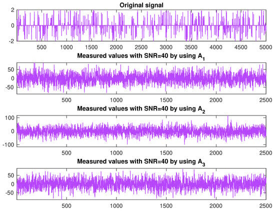
Figure 1. From top to bottom: the original signal and the measurement by using $A_1$, $A_2$ and $A_3$, respectively, with $m=500$.

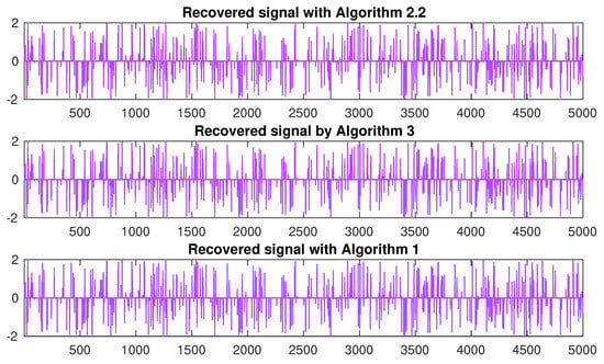
Figure 2. Reconstructed signals obtained using three different algorithms for $m=500$ are displayed from top to bottom. Algorithm 2.2 from [1] and Algorithm 3 from [3].

In these scenarios, it is evident that iteration improves the numerical outcomes. To quantify the differences between these results, we calculate the mean-squared errors of each reconstructed signal in Figure 3. In Table 1, different numbers of nonzero elements are used in the numerical experiments: $m=100,300$, and $500.$ The elapsed periods and number of iterations for each algorithm are recorded. As a consequence of the control parameter settings, we observe that Algorithm 1 uses less time on average than the other algorithms, and has a lower number of iterations. Also, we show the recovery signal results for $m=500$ in Figure 1 and Figure 2.

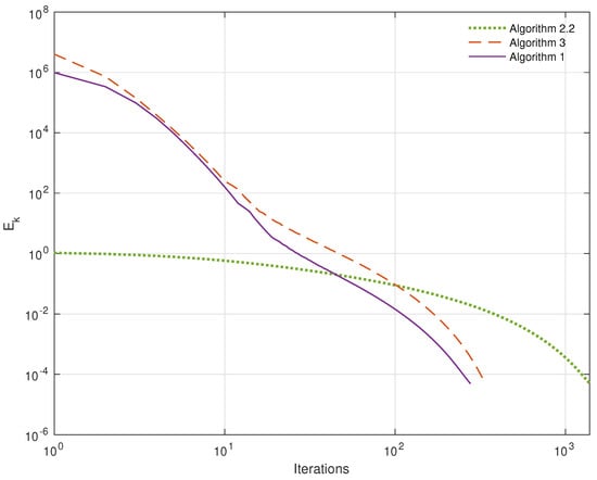
Figure 3. Plots of $E_k$ over iterations when $m=500$. Algorithm 2.2 from [1] and Algorithm 3 from [3].

It is clear that iteration enhances the numerical results. We compute the mean-squared errors of each reconstructed signal in Figure 3 to detect the differences between these outcomes. Figure 4 presents the plot of the structural similarity index measure (SSIM), developed by Wang et al. [41], across iterations. The SSIM value ranges from 0 to 1, where a value of 1 indicates complete signal recovery.

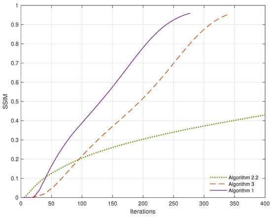
Figure 4. Plots of SSIM over iterations when $m=500$. Algorithm 2.2 from [1] and Algorithm 3 from [3].

5. Conclusions

We develop a novel parallel algorithm for solving the common variational inclusion and common fixed-point (CVI-CFP) problem by integrating inertial and Tseng’s techniques within a variational framework and incorporating fixed-point methods. This method achieves strong convergence, generalizing and improving upon existing results. A strong convergence theorem guarantees its reliability under conditions involving demicontractive and Lipschitz mappings. It is worth noting that the algorithm effectively merges variational inclusion and fixed-point problem solutions. Numerical experiments on signal recovery problems with various blurred filters demonstrate accuracy and efficiency compared with existing methods. This study makes substantial theoretical and practical advancements, providing a valuable tool for solving real-world problems in signal recovery.

References

- Suantai, S.; Kankam, K.; Cholamjiak, P.; Cholamjiak, W. A parallel monotone hybrid algorithm for a finite family of G-nonexpansive mappings in Hilbert spaces endowed with a graph applicable in signal recovery. Comput. Appl. Math. 2021, 40, 145. [Google Scholar] [CrossRef]
- Suparatulatorn, R.; Chaichana, K. A strongly convergent algorithm for solving common variational inclusion with application to image recovery problems. Appl. Numer. Math. 2022, 173, 239–248. [Google Scholar] [CrossRef]
- Mouktonglang, T.; Poochinapan, K.; Suparatulatorn, R. A parallel method for common variational inclusion and common fixed point problems with applications. Carpathian J. Math. 2023, 39, 189–200. [Google Scholar] [CrossRef]
- Lions, P.L.; Mercier, B. Splitting algorithms for the sum of two nonlinear operators. SIAM J. Numer. Anal. 1979, 16, 964–979. [Google Scholar] [CrossRef]
- Passty, G.B. Ergodic convergence to a zero of the sum of monotone operators in Hilbert space. J. Math. Anal. Appl. 1979, 72, 383–390. [Google Scholar] [CrossRef]
- Moudafi, A.; Oliny, M. Convergence of a splitting inertial proximal method for monotone operators. J. Comput. Appl. Math. 2003, 55, 447–454. [Google Scholar] [CrossRef]
- Tseng, P. A modified forward-backward splitting method for maximal monotone mappings. SIAM J. Control. Optim. 2000, 38, 431–446. [Google Scholar] [CrossRef]
- Lorenz, D.A.; Pock, T. An inertial forward-backward algorithm for monotone inclusions. J. Math. Imaging Vis. 2015, 51, 311–325. [Google Scholar] [CrossRef]
- Cholamjiak, W.; Cholamjiak, P.; Suantai, S. An inertial forward-backward splitting method for solving inclusion problems in Hilbert spaces. J. Fixed Point Theory Appl. 2018, 30, 42. [Google Scholar] [CrossRef]
- Gibali, A.; Thong, D.V. Tseng type methods for solving inclusion problems and its applications. Calcolo 2018, 55, 49. [Google Scholar] [CrossRef]
- Abubakar, J.; Kumam, P.; Garba, A.I.; Abdullahi, M.S.; Ibrahim, A.H.; Sitthithakerngkiet, K. An inertial iterative scheme for solving variational inclusion with application to Nash-Cournot equilibrium and image restoration problems. Carpathian J. Math. 2021, 37, 361–380. [Google Scholar] [CrossRef]
- Cholamjiak, P.; Hieu, D.V.; Cho, Y.J. Relaxed forward-backward splitting methods for solving variational inclusions and applications. J. Sci. Comput. 2021, 88, 85. [Google Scholar] [CrossRef]
- Suparatulatorn, R.; Cholamjiak, W.; Gibali, A.; Mouktonglang, T. A parallel Tseng’s splitting method for solving common variational inclusion applied to signal recovery problems. Adv. Differ. Equ. 2021, 2021, 492. [Google Scholar] [CrossRef]
- Suantai, S.; Cholamjiak, W.; Cholamjiak, P. Strong convergence theorems of a finite family of quasi-nonexpansive and Lipschitz multi-valued mappings. Afr. Mat. 2015, 26, 345–355. [Google Scholar] [CrossRef]
- Anh, P.K.; Hieu, D.V. Parallel and sequential hybrid methods for a finite family of asymptotically quasi ϕ-nonexpansive mappings. J. Appl. Math. Comput. 2015, 48, 241–263. [Google Scholar] [CrossRef]
- Cholamjiak, W.; Khan, S.A.; Yambangwai, D.; Kazmi, K.R. Strong convergence analysis of common variational inclusion problems involving an inertial parallel monotone hybrid method for a novel application to image restoration. Revista de la Real Academia de Ciencias Exactas. Físicas Nat. Ser. A Matemát. 2020, 114, 99. [Google Scholar]
- Eslamian, M. Strong convergence theorem for common zero points of inverse strongly monotone mappings and common fixed points of generalized demimetric mappings. Optimization 2021, 71, 4265–4287. [Google Scholar] [CrossRef]
- Eslamian, M.; Kamandi, A. A novel algorithm for approximating common solution of a system of monotone inclusion problems and common fixed point problem. J. Ind. Manag. Optim. 2021, 19, 868–889. [Google Scholar] [CrossRef]
- Wairojjana, N.; Younis, M.; Rehman, H.U.; Pakkaranang, N.; Pholasa, N. Modified viscosity subgradient extragradient-like algorithms for solving monotone variational inequalities problems. Axioms 2020, 9, 118. [Google Scholar] [CrossRef]
- Antón-Sancho, Á. Fixed points of automorphisms of the vector bundle moduli space over a compact Riemann surface. Mediterr. J. Math. 2024, 21, 20. [Google Scholar] [CrossRef]
- Beck, A.; Teboulle, M. A fast iterative shrinkage-thresholding algorithm for linear inverse problems. SIAM J. Imaging Sci. 2009, 2, 183–202. [Google Scholar] [CrossRef]
- Shehu, Y.; Cholamjiak, P. Iterative method with inertial for variational inequalities in Hilbert spaces. Calcolo 2019, 56, 4. [Google Scholar] [CrossRef]
- Mouktonglang, T.; Suparatulatorn, R. Inertial hybrid projection methods with selection techniques for split common fixed point problems in Hilbert spaces. Univ. Politeh. Buchar. Sci. Bull. Ser. A 2022, 54, 47–54. [Google Scholar]
- Kesornprom, S.; Cholamjiak, P. A modified inertial proximal gradient method for minimization problems and applications. AIMS Math. 2022, 7, 8147–8161. [Google Scholar] [CrossRef]
- Peeyada, P.; Suparatulatorn, R.; Cholamjiak, W. An inertial Mann forward-backward splitting algorithm of variational inclusion problems and its applications. Chaos Solitons Fractals 2022, 158, 112048. [Google Scholar] [CrossRef]
- Kabukçuoğlu, A.; Martínez-García, E. A Generalized Time Iteration Method for Solving Dynamic Optimization Problems with Occasionally Binding Constraints. Comput. Econ. 2021, 58, 435–460. [Google Scholar] [CrossRef]
- Zheng, T.; Bergin, M.H.; Hu, S.; Carlson, D.E. Estimating ground-level PM2.5 using micro-satellite images by a convolutional neural network and random forest approach. Atmos. Environ. 2020, 230, 117451. [Google Scholar] [CrossRef]
- Doreswamy, H.; Harishkumar, K.S.; Yogesh, K.M.; Ibrahim, G. Forecasting Air Pollution Particulate Matter (PM2.5) Using Machine Learning Regression Models. Procedia Comput. Sci. 2020, 171, 2057–2066. [Google Scholar] [CrossRef]
- Gokul, P.R.; Mathew, A.; Bhosale, A.; Nair, A.T. Spatio-temporal air quality analysis and PM2.5 prediction over Hyderabad City, India using artificial intelligence techniques. Ecol. Inform. 2023, 76, 102067. [Google Scholar] [CrossRef]
- Mathew, A.; Gokul, P.R.; Raja Shekar, P.; Arunab, K.S.; Ghassan Abdo, H.; Almohamad, H.; Abdullah Al Dughairi, A. Air quality analysis and PM2.5 modelling using machine learning techniques: A study of Hyderabad city in India. Cogent Eng. 2023, 10, 2243743. [Google Scholar] [CrossRef]
- Xu, H.K. Iterative algorithms for nonlinear operators. J. Lond. Math. Soc. 2002, 66, 240–256. [Google Scholar] [CrossRef]
- Maingé, P.E. Strong convergence of projected subgradient methods for nonsmooth and nonstrictly convex minimization. Set-Valued Anal. 2008, 16, 899–912. [Google Scholar] [CrossRef]
- Goebel, K.; Kirk, W. Topics in Metric Fixed Point Theory; Cambridge Studies in Advanced Mathematics; Cambridge University Press: Cambridge, UK, 1990; Volume 28. [Google Scholar]
- Marino, G.; Xu, H.K. Weak and strong convergence theorems for strict pseudo-contractions in Hilbert spaces. J. Math. Anal. Appl. 2007, 329, 336–346. [Google Scholar] [CrossRef]
- Browder, F.E. Nonlinear maximal monotone operators in Banach space. Math. Ann. 1968, 175, 89–113. [Google Scholar] [CrossRef]
- Bauschke, H.H.; Combettes, P.L. Convex Analysis and Monotone Operator Theory in Hilbert Spaces; CMS Books in Mathematics: New York, NY, USA, 2011. [Google Scholar]
- Brézis, H. Opérateurs Maximaux Monotones et Semi-groupes de Contractions dans les Espaces de Hilbert; Mathematical Studies: Amsterdam, The Netherlands, 1973; Volume 5. [Google Scholar]
- Tan, B.; Zhou, Z.; Li, S. Viscosity-type inertial extragradient algorithms for solving variational inequality problems and fixed point problems. J. Appl. Math. Comput. 2022, 68, 1387–1411. [Google Scholar] [CrossRef]
- Liu, H.; Yang, J. Weak convergence of iterative methods for solving quasimonotone variational inequalities. Comput. Optim. Appl. 2020, 77, 491–508. [Google Scholar] [CrossRef]
- Combettes, P.L.; Wajs, V.R. Signal recovery by proximal forward-backward splitting. Multiscale Model. Simul. 2005, 4, 1168–1200. [Google Scholar] [CrossRef]
- Wang, Z.; Bovik, A.C.; Sheikh, H.R.; Simoncelli, E.P. Image quality assessment: From error visibility to structural similarity. IEEE Trans. Image Process. 2004, 13, 600–612. [Google Scholar] [CrossRef]
Disclaimer/Publisher’s Note: The statements, opinions and data contained in all publications are solely those of the individual author(s) and contributor(s) and not of MDPI and/or the editor(s). MDPI and/or the editor(s) disclaim responsibility for any injury to people or property resulting from any ideas, methods, instructions or products referred to in the content. |
© 2024 by the authors. Licensee MDPI, Basel, Switzerland. This article is an open access article distributed under the terms and conditions of the Creative Commons Attribution (CC BY) license (https://creativecommons.org/licenses/by/4.0/).