A Heuristic Attribute-Reduction Algorithm Based on Conditional Entropy for Incomplete Information Systems

Abstract

With the continuous expansion of databases, the extraction of information has been an urgent research topic in many fields. As an effective method to remove redundant attributes, attribute reduction demonstrates extraordinary ability in simplifying information systems. This paper applies a novel form of conditional entropy to investigate the attribute reduction in incomplete information systems. Firstly, a novel definition of conditional entropy is introduced based on tolerance relation. Additionally, in order to reduce time complexity, we propose a binsearch heuristic attribute-reduction algorithm with conditional entropy as heuristic knowledge. Furthermore, two examples are used to illustrate the feasibility and validity of the reduction algorithm.

1. Introduction

      Human society has been in the era of network information for many years. How to efficiently extract useful information from information systems with massive data has become a hot and difficult topic in big data analysis and machine learning. Sometimes, the data are incomplete and many redundant attributes exist in an information system. How to reduce the number of redundant attributes without changing classification ability is a tricky question in many fields. Fortunately, attribute reduction, as one of the core contents of a rough set, can reduce redundant attributes effectively and has been studied by many researchers [1,2,3,4,5,6,7,8]. Attribute-reduction methods for complete information systems have been well established; however, there are limitations in dealing with attribute-reduction problems in incomplete information systems since the objects with missing data cannot be classified effectively by an equivalence relation. Therefore, developing reliable attribute-reduction methods in incomplete information systems is an important direction for current research [9,10,11].

So far, there exist two main kinds of algorithms for attribute reduction. One is the discernibility matrix-based method proposed by Skowron [12]. In recent years, Liu et al. [13,14,15] published several works about attribute-reduction algorithms based on discernibility matrix, but the high time complexity in transforming a conjunctive normal form into a disjunctive normal form has always been a problem. Although the time complexity of this algorithm is high, it can obtain all reducts. The other is the heuristic algorithm, which has low time complexity and is effective for large data sets, but it can only obtain one reduct, not all reducts. For information systems with a large number of attributes, a heuristic algorithm is a better choice. Heuristic knowledge is a core element for heuristic algorithms, so it is crucial to use appropriate heuristic knowledge to obtain an accurate reduct. In many heuristic algorithms, attribute significance is usually adopted, as heuristic knowledge and information entropy are the most-favored choices to measure attribute significance, such as Shannon entropy [16], joint maximum entropy [17], and relative decision entropy [18]. Specifically, Dai et al. [19] introduced a novel form of conditional entropy to calculate attribute significance and further constructed three attribute-selection algorithms from the viewpoint of exhaustive search, greedy (heuristic) search, and probabilistic search for incomplete decision systems. To reduce the complexity of attribute-reduction algorithms, Thuy and Wongthanavasu [20] adopted stripped-quotient sets to identify several reducts based on information entropies. However, only one candidate attribute can be tested at a time in their algorithms. Zou et al. [21] employed a supervised strategy to update the conditional neighborhood entropy of three-layer granulation and considered the mutual influence between conditional attributes, then proposed a neighborhood rough set attribute-reduction algorithm. Chen and Zhu [22] proposed variable-precision multigranulation rough sets (VPMGRSs) and designed a heuristic algorithm to incorporate the $\alpha$ lower distribution reduct into the multigranulation environment. On the other hand, to reduce time complexity, Zhou et al. [23] designed a binsearch heuristic algorithm based on attribute significance, in which the attribute significance is measured with the help of a similarity matrix. It turns out that the idea of binsearch can effectively reduce the time complexity of attribute reduction. Until now, the research about binsearch heuristic algorithm has been scarce.

In summary, algorithms based on the discernibility matrix can identify all reductions, but they have high time complexity when transforming data representations. On the other hand, heuristic algorithms generally have higher computational efficiency and are suitable for large datasets. However, they are limited to identifying only one reduction and cannot capture the full complexity of the dataset. Therefore, this paper proposes a novel form of conditional entropy as heuristic knowledge and combines the idea of binsearch to investigate the attribute-reduction algorithm in incomplete information systems.

The remainder of this paper is organized as follows. In Section 2, we review some basic definitions and give the calculation method of conditional entropy based on the tolerance relation. In Section 3, the method for acquiring core attributes and the binsearch heuristic attribute-reduction algorithm are proposed. In Section 4, two examples are given to illustrate the feasibility and availability of our algorithm. Section 5 concludes the paper.

2. Preliminaries

In this section, we recall some basic definitions about incomplete information systems, tolerance relations, and conditional entropy.

Definition 1

([23]). Let $U=\{x_1,x_2,\cdots ,x_n\}$ be an object set, $A=\{a_1,a_2,\cdots ,a_m\}$ be an attribute set, and f: $U\times A\to V$ be an information function. The value set is defined as ${\displaystyle V={\cup }_{a\in A}{V}_a}$, where $V_a$ represents the set of evaluation values of all objects associated with attribute $a\in A$. Then, $S=(U,A,f,V)$ is called an information system. If there exist $a\in A,x\in U$ such that $f(x,a)=\ast$, where “∗” represents missing value, then $S=(U,A,f,V)$ is an incomplete information system.

Sometimes, $S=(U,A,f,V)$ is abbreviated as $S=(U,A)$—as long as there are no confusions. If $A=C\cup D$ and $C\cap D=\varnothing$, then $(U,C\cup D)$ is called a decision information system, where C and D are termed as the condition attribute set and decision attribute set, respectively.

In incomplete information systems, an equivalence relation is often not effective in categorizing objects since missing data make it difficult to recognize the similarity between objects. To classify objects effectively in incomplete information systems, a tolerance relation is introduced. It regards objects as similar if they have the same values under all attributes with complete data. The specific definition is as follows.

Definition 2

([12]). Suppose that $S=(U,A)$ is an incomplete information system, $C\subseteq A$; for any $x,y\in U$, tolerance relation $R_C$ is defined as

$$R_C=\left\{(x,y)\right|\forall a\in C,f(x,a)=f(y,a)\mathit{or}f(x,a)=\ast \mathit{or}f(y,a)=\ast \}.$$

In many situations, $f(x,a)$ is also denoted as $a\left(x\right)$ for simplicity. Obviously, $R_C$ is reflexive and symmetric, but not necessarily transitive, and $U/R_C=\{R_C\left(x_1\right),R_C\left(x_2\right),\cdots ,$ $R_C\left(x_{\left|U\right|}\right)\}(x_i\in U)$ is a covering of U, where $R_C\left(x_i\right)=\{y\in U|(x_i,y)\in R_C)\}$ represents the tolerance class of $x_i$ with respect to C. Let $U_{CD}=\left\{x\right|R_C\left(x\right)\subseteq R_D\left(x\right)\}$; then, $U_{CD}$ is called the consistent part of $(U,C\cup D)$ [24].

Theorem 1.

Let $S=(U,C\cup D)$ be an incomplete information system. If $T\subseteq C$, then $U_{TD}\subseteq U_{CD}$.

Proof. 

Since $T\subseteq C$, we can have $R_C\left(x\right)\subseteq R_T\left(x\right)$ for any $x\in U$. If $x^{\prime }\in U_{TD}$, then $R_T\left(x^{\prime }\right)\subseteq R_D\left(x^{\prime }\right)$. Furthermore, $R_C\left(x^{\prime }\right)\subseteq R_D\left(x^{\prime }\right)$. Thus, $x^{\prime }\in U_{CD}$. Therefore, we can obtain $U_{TD}\subseteq U_{CD}$.    □

Definition 3

([24]). Suppose that $S=(U,C\cup D)$ is an incomplete decision information system, $\varnothing \ne T\subseteq C$. If T satisfies the following conditions:

(1) $U_{TD}=U_{CD}$;

(2) For any $\varnothing \ne T^{\prime }\subset T$, $U_{T^{\prime }D}\ne U_{CD}$;

then T is called a reduct of C.

It should be noticed that there may be many different attribute reducts for an information system, and the attributes that appear in all reducts are called core attributes.

Information entropy, proposed by Shannon [25], refers to the average uncertainty of information sources, also known as unconditional entropy. When some certain conditions affect the probability distribution of information sources, they may affect the uncertainty of information sources, so conditional entropy appears. Conditional entropy represents the conditional uncertainty of one event under another event [26]. The smaller the conditional entropy, the smaller the conditional uncertainty of one event with respect to another event, and vice versa. Thuy  [20] gave a calculation method of conditional entropy for complete information systems.

Definition 4

([20]). In a complete information system $S=(U,C\cup D)$, the conditional entropy of D with respect to C is defined as

$$H\left(D\right|C)=-\sum _{X\in U/C}{\displaystyle \frac{\left|X\right|}{\left|U\right|}}\sum _{Y\in U/D}{\displaystyle \frac{|X\cap Y|}{\left|X\right|}}log{\displaystyle \frac{|X\cap Y|}{\left|X\right|}},$$

where $U/C$ denotes the partition of U with respect to C and $U/D$ denotes the partition of U with respect to D.

The above definition suggests that conditional entropy is the extent to which uncertainty about another variable $\left(Y\right)$ is reduced after some of the information $\left(X\right)$ is known. $H\left(D\right|C)$ denotes the uncertainty of D under condition C. The smaller the value of $H\left(D\right|C)$, the smaller the uncertainty of D under condition C, and vice versa. Then, $H\left(D\right|\left\{a_i\right\})(\forall a_i\in C,i=1,2,\cdots ,\left|C\right|)$ denotes the conditional entropy of D with respect to condition attribute $a_i$. The smaller the value of $H\left(D\right|\left\{a_i\right\})$, the smaller the uncertainty of D under condition attribute $a_i$, indicating that attribute $a_i$ is more significant in a system. Therefore, we can determine the significance of an attribute in an information system according to its conditional entropy, i.e., conditional entropy can be used as the heuristic knowledge in the process of attribute reduction.

When dealing with the attribute-reduction problem of a complete information system, the conditional entropy defined in Definition 5 is often adopted, but it is not suitable for incomplete information systems. To overcome this difficulty, we define a novel form of conditional entropy based on the tolerance relation as follows.

Definition 5.

Given an incomplete information system $S=(U,C\cup D)$, the conditional entropy of D with respect to C is defined as

$$H\left(D\right|C)=-\sum _{i=1}^{\left|U\right|}{\displaystyle \frac{|R_C\left(x_i\right)|}{\left|U\right|}}\sum _{j=1}^{|U/D|}{\displaystyle \frac{|R_C\left(x_i\right)\cap D_j|}{|R_C\left(x_i\right)|}}log{\displaystyle \frac{|R_C\left(x_i\right)\cap D_j|}{|R_C\left(x_i\right)|}}.$$

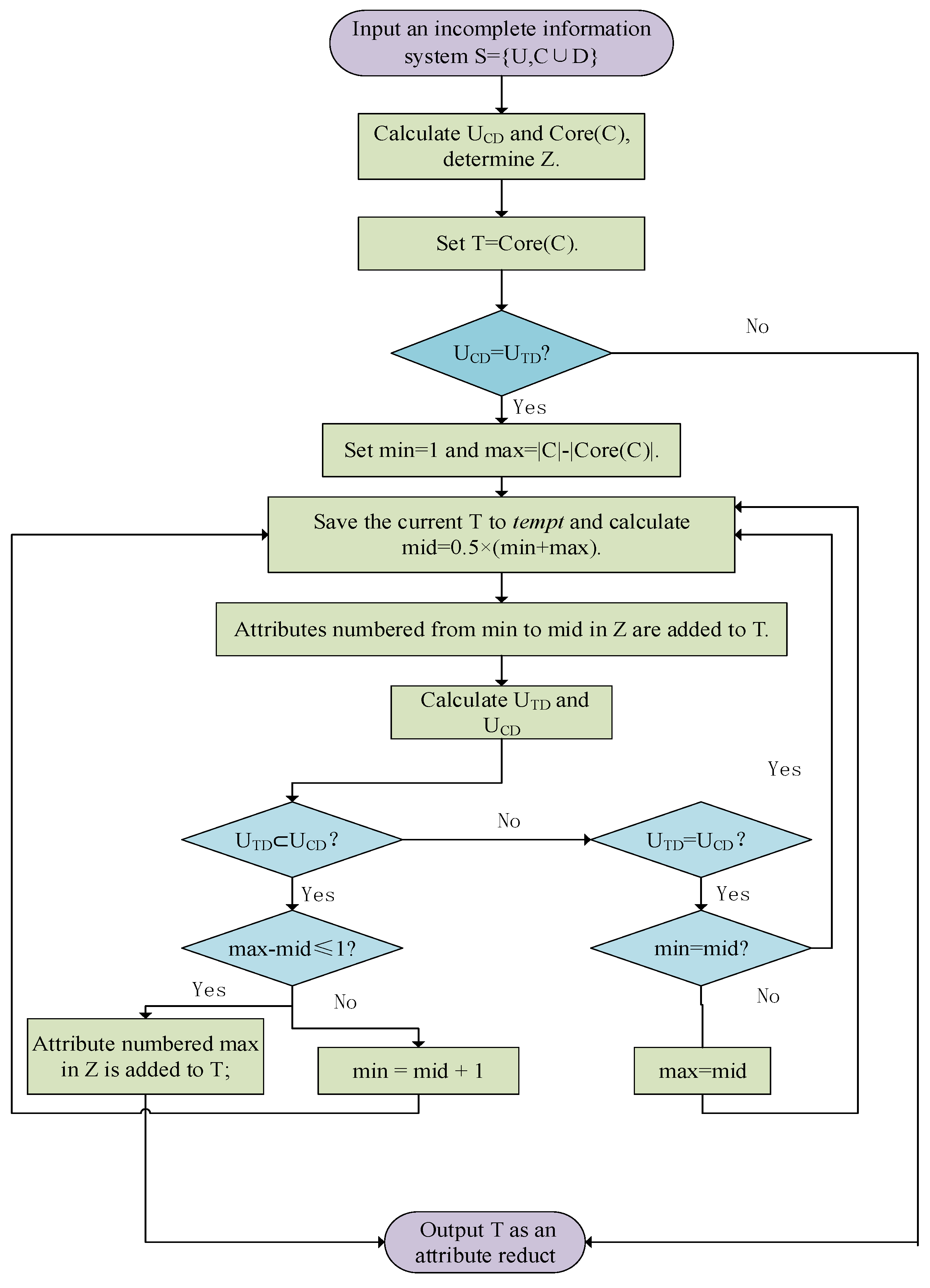
3. Binsearch Heuristic Reduction Algorithm Based on Conditional Entropy

In order to reduce time complexity and space complexity, many heuristic reduction algorithms start from core attributes. Thus, determining the core attributes of an information system is of great significance. Next, we give a sufficient condition to determine the core attributes of an incomplete decision system.

Theorem 2.

Given an incomplete decision system $S=(U,C\cup \{d\left\}\right)$, for objects $x_i$, $x_j\in U$$(x_i\ne x_j)$, if $d\left(x_i\right)\ne d\left(x_j\right)$, $min\left\{\right|{\sigma }_C\left(x_i\right)|,|{\sigma }_C\left(x_j\right)\left|\right\}=1$$({\sigma }_C\left(x_i\right)=\{d\left(y\right),y\in R_C\left(x_i\right)\})$, and only one $a_k(a_k\in C)$ satisfies the condition $a_k\left(x_i\right)\ne a_k\left(x_j\right)$, then $a_k$ is a core attribute, i.e., $a_k\in core\left(C\right)$.

Proof. 

Let $D=\left\{d\right\}$. Consider $min\left\{\right|{\sigma }_C\left(x_i\right)|,|{\sigma }_C\left(x_j\right)\left|\right\}=1$. If $|{\sigma }_C\left(x_j\right)|=1$, then $R_C\left(x_j\right)\subseteq R_{\left\{d\right\}}\left(x_j\right)$, so $x_j\in U_{CD}$. If $|{\sigma }_C\left(x_i\right)|=1$, then $R_C\left(x_i\right)\subseteq R_{\left\{d\right\}}\left(x_i\right)$, so $x_i\in U_{CD}$. In addition, since there is only one attribute $a_k(a_k\in C)$ satisfying $a_k\left(x_i\right)\ne a_k\left(x_j\right)$, so $a_l\left(x_i\right)=a_l\left(x_j\right)(a_l\in (C-\left\{a_k\right\})$, and $x_j\notin R_C\left(x_i\right)$, $x_i\notin R_C\left(x_j\right)$. Let $E=C-\left\{a_k\right\}$; then, $x_j\in R_E\left(x_i\right)$, $x_i\in R_E\left(x_j\right)$. Since $d\left(x_i\right)\ne d\left(x_j\right)$, it can be observed that $x_j\notin R_{\left\{d\right\}}\left(x_i\right)$ and $x_i\notin R_{\left\{d\right\}}\left(x_j\right)$. $U_{ED}=\left\{x\right|R_E\left(x\right)\subseteq R_{\left\{d\right\}}\left(x\right)\}$, which means that $x_i\notin U_{ED}$ and $x_j\notin U_{ED}$. Then, $U_{ED}⫋U_{CD}$. Therefore, $a_k\in core\left(C\right)$.    □

Example 1.

Suppose that $S=(U,C\cup \{d\left\}\right)$ is an incomplete decision table (as shown in

Table 1. Incomplete decision Table 1.

	${\mathit{a}}_1$	${\mathit{a}}_2$	${\mathit{a}}_3$	${\mathit{a}}_4$	d
$x_1$	2	3	2	0	1
$x_2$	∗	2	∗	1	2
$x_3$	∗	2	∗	1	1
$x_4$	2	3	2	1	1
$x_5$	3	∗	∗	3	2
$x_6$	∗	0	0	∗	1
$x_7$	3	2	1	3	1
$x_8$	1	∗	∗	∗	2

), $U=\{x_1,x_2,\cdots ,x_8\}$, $C=\{a_1,a_2,a_3,a_4\}$, and $D=\left\{d\right\}$. The numbers in Table 1 indicate scores for each decision alternative, while ★ signifies missing values. The core attributes can be obtained as follows.

Firstly, it can be seen that object pairs that satisfy condition $d\left(x_i\right)\ne d\left(x_j\right)$ are $(x_1,x_2)$, $(x_1,x_5)$, $(x_1,x_8)$, $(x_2,x_3)$, $(x_2,x_4)$, $(x_2,x_6)$, $(x_2,x_7)$, $(x_3,x_5)$, $(x_3,x_8)$, $(x_4,x_5)$, $(x_4,x_8)$, $(x_5,x_6)$, $(x_5,x_7)$, $(x_6,x_8)$, $(x_7,x_8)$.

Secondly, we can observe that $R_C\left(x_1\right)=\left\{x_1\right\}$, $R_C\left(x_2\right)=\{x_2,x_3\}$, $R_C\left(x_3\right)=\{x_2,x_3\}$, $R_C\left(x_4\right)=\left\{x_4\right\}$, $R_C\left(x_5\right)=\{x_5,x_6,x_7\}$, $R_C\left(x_6\right)=\{x_5,x_6\}$, $R_C\left(x_7\right)=\{x_5,x_7\}$, $R_C\left(x_8\right)=\{x_2,x_3,x_6,x_8\}$. Accordingly, $\sigma \left(x_1\right)=\left\{1\right\}$, $\sigma \left(x_2\right)=\{1,2\}$, $\sigma \left(x_3\right)=\{1,2\}$, $\sigma \left(x_4\right)=\left\{1\right\}$, $\sigma \left(x_5\right)=\{1,2\}$, $\sigma \left(x_6\right)=\{1,2\}$, $\sigma \left(x_7\right)=\{1,2\}$, $\sigma \left(x_8\right)=\{1,2\}$. Thus, all the object pairs that satisfy conditions $d\left(x_i\right)\ne d\left(x_j\right)$ and $min\left\{\right|\sigma \left(x_i\right)|,|\sigma \left(x_j\right)\left|\right\}=1$ are $(x_1,x_2),(x_1,x_5),(x_1,x_8),$$(x_2,x_4),(x_4,x_5),(x_4,x_8)$.

Thirdly, it is obvious that objects $x_1$ and $x_2$ can be distinguished by $a_2$ and $a_4$, objects $x_1$ and $x_5$ can be distinguished by $a_1$ and $a_4$, objects $x_2$ and $x_4$ can be distinguished by $a_2$, objects $x_4$ and $x_5$ can be distinguished by $a_1$ and $a_4$, objects $x_1$ and $x_8$ can be distinguished by $a_1$, and objects $x_4$ and $x_8$ can be distinguished by $a_1$.

Consequently, $a_1$ and $a_2$ are core attributes, i.e., $core\left(C\right)=\{a_1,a_2\}$.

In fact, the essence of attribute reduction is to obtain the smallest $T(T\subseteq C)$ such that $U_{TD}=U_{CD}$. Next, we apply the idea of binsearch to propose a heuristic attribute-reduction algorithm based on conditional entropy to obtain T. The process of Algorithm 1 and the corresponding Figure 1 are shown below.

Algorithm 1 Process of the binsearch heuristic reduction algorithm based on conditional entropy

Input: An incomplete information system $S=(U,C\cup D)$. Output: A reduct T of C. Step 1: Calculate $U_{CD}$. $core\left(C\right)$ is obtained by Theorem 2; other remaining attributes are placed in ascending order in a candidate attribute set Z according to their conditional entropies. Step 2: Initialization: $T=core\left(C\right)$; if $U_{TD}=U_{CD}$, then go to Step 4, else go to Step 3. Step 3: Initialization: $min=1$, $max=\left|C\right|$−$\left|core\right(C\left)\right|$. while (true) do    $tempt=T$; // Save T before making the change.    ${\displaystyle \mathrm{mid}=\left[\frac{min+max}{2}\right]}$;    Attributes numbered from min to $\mathrm{mid}$ in Z are added to T. Then, calculate $U_{TD}$ and $U_{CD}$.    if $(U_{TD}\subset U_{CD})$ then       if $(max-\mathrm{mid}\le 1)$ then          (1) Attribute numbered max in Z is added to T;          (2) Exit the cycle; // End of the algorithm.       else          $min=\mathrm{mid}+1$; // Enter the next cycle.       end if    else $(U_{TD}=U_{CD})$ then       if $(min=\mathrm{mid})$ then          (3) Exit the cycle; // End of the algorithm.       else          (4) $max=\mathrm{mid}$;          $T=tempt$; // Restore T to its previous state, and enter the next cycle.       end if    end if end while Step 4: End of the algorithm.

This algorithm is designed to reduce the time complexity by testing multiple candidate attributes each time. When one half of the attributes in Z are added to T, if $U_{TD}\subset U_{CD}$, this indicates that other attributes need to be added to T, and, if $max-\mathrm{mid}\le 1$, this means that only the attribute numbered max in Z can be added to T. Therefore, the attribute numbered max in Z is directly added to T, and we stop the algorithm. If $max-\mathrm{mid}>1$, which means that attributes with a number larger than $\mathrm{mid}$ should be added to T, then $\mathrm{mid}+1$ is directly assigned to min. When $U_{TD}=U_{CD}$, if $min=\mathrm{mid}$, this indicates that T is the smallest reduct, and we end the algorithm. If $min\ne \mathrm{mid}$, this means that T may not be the smallest reduct. In order to obtain the smallest reduct, let $max=\mathrm{mid}$. The attribute reduction of information systems can be obtained by repeating this computation. Obviously, when adding one half of the attributes in Z to T, if $U_{TD}=U_{CD}$, this implies that the algorithm terminates before an attribute numbered $\mathrm{mid}$ in Z or terminates at the position of $\mathrm{mid}$. If $U_{TD}\subset U_{CD}$, this means that the algorithm terminates after an attribute numbered $\mathrm{mid}$ in Z. It can be seen that, during the process of attribute reduction, our heuristic algorithm can add multiple candidate attributes each time, thereby reducing time complexity.

The time complexity of the conditional entropy-based binary search heuristic reduction algorithm can be summarized as follows. The input phase is completed in $O\left(1\right)$. In Step 1, calculating $U_{CD}$ takes $O\left(mn\right)$ time, where n is the number of attributes and m is the number of attributes. Sorting the attributes takes $O\left(nlogn\right)$, resulting in a total of $O(mn+nlogn)$. In Step 2, initializing T in $O\left(1\right)$ and checking the condition $U_{TD}=U_{CD}$ requires $O\left(mn\right)$ time. Thus, the total time complexity for Step 2 is $O\left(mn\right)$. In Step 3, the binary search runs in $O\left(logn\right)$ iterations, with each iteration requiring $O\left(mn\right)$, leading to a complexity of $O\left(nmlogn\right)$. The termination step is $O\left(1\right)$. In conclusion, the overall time complexity of the algorithm is $O\left(nmlogn\right)$. In addition, the time complexity of the algorithm in [23] is $O\left(n^2\right)$, which is significantly higher than that of our algorithm when dealing with large sample data. This shows that the algorithm in this paper has superior efficiency.

4. Examples

To verify the effectiveness of the proposed algorithm, an incomplete decision table $S=(U,C\cup D)$ (as shown in

Table 2. Incomplete decision Table 2.

	${\mathit{a}}_1$	${\mathit{a}}_2$	${\mathit{a}}_3$	${\mathit{a}}_4$	${\mathit{a}}_5$	${\mathit{a}}_6$	${\mathit{a}}_7$	${\mathit{a}}_8$	d
$x_1$	3	2	1	1	1	0	∗	∗	0
$x_2$	2	3	2	0	∗	1	3	1	0
$x_3$	2	3	2	0	1	∗	3	1	1
$x_4$	∗	2	∗	1	∗	2	0	1	1
$x_5$	∗	2	∗	1	1	2	0	1	1
$x_6$	2	3	2	1	3	1	∗	1	1
$x_7$	3	∗	∗	3	1	0	2	∗	0
$x_8$	∗	0	0	∗	∗	0	2	0	1
$x_9$	3	2	1	3	1	1	2	1	1
$x_{10}$	1	∗	∗	∗	1	0	∗	0	0
$x_{11}$	∗	2	∗	∗	1	∗	0	1	0
$x_{12}$	3	2	1	∗	∗	0	2	3	0

) from reference [23] is adopted. Next, we apply the binsearch heuristic algorithm to obtain a reduct of C.

Example 2.

An incomplete decision table $S=(U,C\cup \{d\left\}\right)$ is shown in Table 2, where $U=\{x_1,x_2,\cdots ,x_{12}\}$, $C=\{a_1,a_2,\cdots ,a_8\}$. We can obtain a reduct of C as follows:

Step 1. We first use a Boolean matrix to calculate $U_{CD}$. According to Table 2, the Boolean relation matrices of $R_{\left\{a_1\right\}},R_{\left\{a_2\right\}},\cdots ,R_{\left\{a_8\right\}}$, and $R_{\left\{d\right\}}$ can be acquired as follows:

$$M_{R_{\left\{a_1\right\}}}={\left[\begin{array}{cccccccccccc}1& 0& 0& 1& 1& 0& 1& 1& 1& 0& 1& 1\\ 0& 1& 1& 1& 1& 1& 0& 1& 0& 0& 1& 0\\ 0& 1& 1& 1& 1& 1& 0& 1& 0& 0& 1& 0\\ 1& 1& 1& 1& 1& 1& 1& 1& 1& 1& 1& 1\\ 1& 1& 1& 1& 1& 1& 1& 1& 1& 1& 1& 1\\ 0& 1& 1& 1& 1& 1& 0& 1& 0& 0& 1& 0\\ 1& 0& 0& 1& 1& 0& 1& 1& 1& 0& 1& 1\\ 1& 1& 1& 1& 1& 1& 1& 1& 1& 1& 1& 1\\ 1& 0& 0& 1& 1& 0& 1& 1& 1& 0& 1& 1\\ 0& 0& 0& 1& 1& 0& 0& 1& 0& 1& 1& 0\\ 1& 1& 1& 1& 1& 1& 1& 1& 1& 1& 1& 1\\ 1& 0& 0& 1& 1& 0& 1& 1& 1& 0& 1& 1\end{array}\right]}_{12\times 12},M_{R_{\left\{a_2\right\}}}={\left[\begin{array}{cccccccccccc}1& 0& 0& 1& 1& 0& 1& 0& 1& 1& 1& 1\\ 0& 1& 1& 0& 0& 1& 1& 0& 0& 1& 0& 0\\ 0& 1& 1& 0& 0& 1& 1& 0& 0& 1& 0& 0\\ 1& 0& 0& 1& 1& 0& 1& 0& 1& 1& 1& 1\\ 1& 0& 0& 1& 1& 0& 1& 0& 1& 1& 1& 1\\ 0& 1& 1& 0& 0& 1& 1& 0& 0& 1& 0& 0\\ 1& 1& 1& 1& 1& 1& 1& 1& 1& 1& 1& 1\\ 0& 0& 0& 0& 0& 0& 1& 1& 0& 1& 0& 0\\ 1& 0& 0& 1& 1& 0& 1& 0& 1& 1& 1& 1\\ 1& 1& 1& 1& 1& 1& 1& 1& 1& 1& 1& 1\\ 1& 0& 0& 1& 1& 0& 1& 0& 1& 1& 1& 1\\ 1& 0& 0& 1& 1& 0& 1& 0& 1& 1& 1& 1\end{array}\right]}_{12\times 12},$$

$$M_{R_{\left\{a_3\right\}}}={\left[\begin{array}{cccccccccccc}1& 0& 0& 1& 1& 0& 1& 0& 1& 1& 1& 1\\ 0& 1& 1& 1& 1& 1& 1& 0& 0& 1& 1& 0\\ 0& 1& 1& 1& 1& 1& 1& 0& 0& 1& 1& 0\\ 1& 1& 1& 1& 1& 1& 1& 1& 1& 1& 1& 1\\ 1& 1& 1& 1& 1& 1& 1& 1& 1& 1& 1& 1\\ 0& 1& 1& 1& 1& 1& 1& 0& 0& 1& 1& 0\\ 1& 1& 1& 1& 1& 1& 1& 1& 1& 1& 1& 1\\ 0& 0& 0& 1& 1& 0& 1& 1& 0& 1& 1& 0\\ 1& 0& 0& 1& 1& 0& 1& 0& 1& 1& 1& 1\\ 1& 1& 1& 1& 1& 1& 1& 1& 1& 1& 1& 1\\ 1& 1& 1& 1& 1& 1& 1& 1& 1& 1& 1& 1\\ 1& 0& 0& 1& 1& 0& 1& 0& 1& 0& 1& 1\end{array}\right]}_{12\times 12},M_{R_{\left\{a_4\right\}}}={\left[\begin{array}{cccccccccccc}1& 0& 0& 1& 1& 1& 0& 1& 0& 1& 1& 1\\ 0& 1& 1& 0& 0& 0& 0& 1& 0& 1& 1& 1\\ 0& 1& 1& 0& 0& 0& 0& 1& 0& 1& 1& 1\\ 1& 0& 0& 1& 1& 1& 0& 1& 0& 1& 1& 1\\ 1& 0& 0& 1& 1& 1& 0& 1& 0& 1& 1& 1\\ 1& 0& 0& 1& 1& 1& 0& 1& 0& 1& 1& 1\\ 0& 0& 0& 0& 0& 0& 1& 1& 1& 1& 1& 1\\ 1& 1& 1& 1& 1& 1& 1& 1& 1& 1& 1& 1\\ 0& 0& 0& 0& 0& 0& 1& 1& 1& 1& 1& 1\\ 1& 1& 1& 1& 1& 1& 1& 1& 1& 1& 1& 1\\ 1& 1& 1& 1& 1& 1& 1& 1& 1& 1& 1& 1\\ 1& 1& 1& 1& 1& 1& 1& 1& 1& 1& 1& 1\end{array}\right]}_{12\times 12},$$

$$⋮⋮$$

$$M_{R_{\left\{d\right\}}}={\left[\begin{array}{cccccccccccc}1& 1& 0& 0& 0& 0& 1& 0& 0& 1& 1& 1\\ 1& 1& 0& 0& 0& 0& 1& 0& 0& 1& 1& 1\\ 0& 0& 1& 1& 1& 1& 0& 1& 1& 0& 0& 0\\ 0& 0& 1& 1& 1& 1& 0& 1& 1& 0& 0& 0\\ 0& 0& 1& 1& 1& 1& 0& 1& 1& 0& 0& 0\\ 0& 0& 1& 1& 1& 1& 0& 1& 1& 0& 0& 0\\ 1& 1& 0& 0& 0& 0& 1& 0& 0& 1& 1& 1\\ 0& 0& 1& 1& 1& 1& 0& 1& 1& 0& 0& 0\\ 0& 0& 1& 1& 1& 1& 0& 1& 1& 0& 0& 0\\ 1& 1& 0& 0& 0& 0& 1& 0& 0& 1& 1& 1\\ 1& 1& 0& 0& 0& 0& 1& 0& 0& 1& 1& 1\\ 1& 1& 0& 0& 0& 0& 1& 0& 0& 1& 1& 1\end{array}\right]}_{12\times 12},\underset{i=1}{\overset{8}{\bigwedge }}{M}_{R_{\left\{a_i\right\}}}={\left[\begin{array}{cccccccccccc}1& 0& 0& 0& 0& 0& 0& 0& 0& 0& 1& 1\\ 0& 1& 1& 0& 0& 0& 0& 0& 0& 0& 0& 0\\ 0& 1& 1& 0& 0& 0& 0& 0& 0& 0& 0& 0\\ 0& 0& 0& 1& 1& 0& 0& 0& 0& 0& 1& 0\\ 0& 0& 0& 1& 1& 0& 0& 0& 0& 0& 1& 0\\ 0& 0& 0& 0& 0& 1& 0& 0& 0& 0& 0& 0\\ 0& 0& 0& 0& 0& 0& 1& 1& 0& 0& 0& 1\\ 0& 0& 0& 0& 0& 0& 1& 1& 0& 1& 0& 0\\ 0& 0& 0& 0& 0& 0& 0& 0& 1& 0& 0& 0\\ 0& 0& 0& 0& 0& 0& 0& 1& 0& 1& 0& 0\\ 1& 0& 0& 1& 1& 0& 0& 0& 0& 0& 1& 0\\ 1& 0& 0& 0& 0& 0& 1& 0& 0& 0& 0& 1\end{array}\right]}_{12\times 12}.$$

It is easy to obtain $R_C\left(x_1\right)=\{x_1,x_{11},x_{12}\}$, $R_C\left(x_2\right)=R_C\left(x_3\right)=\{x_2,x_3\}$, $R_C\left(x_4\right)=R_C\left(x_5\right)=\{x_4,x_5,x_{11}\}$, $R_C\left(x_6\right)=\left\{x_6\right\}$, $R_C\left(x_7\right)=\{x_7,x_8,x_{12}\}$, $R_C\left(x_8\right)=\{x_7,x_8,x_{10}\}$, $R_C\left(x_9\right)=\left\{x_9\right\}$, $R_C\left(x_{10}\right)=\{x_8,x_{10}\}$, $R_C\left(x_{11}\right)=\{x_1,x_4,x_5,x_{11}\}$, $R_C\left(x_{12}\right)=\{x_1,x_7,x_{12}\}$ from matrix ${\bigwedge }_{i=1}^8{M}_{R_{\left\{a_i\right\}}}$. Similarly, we obtain $R_{\left\{d\right\}}\left(x_1\right)=\{x_1,x_2,x_7,x_{10},x_{11},x_{12}\}$, $R_{\left\{d\right\}}\left(x_2\right)=\{x_1,x_2,x_7,x_{10},x_{11},x_{12}\}$, $R_{\left\{d\right\}}\left(x_3\right)=\{x_3,x_4,x_5,x_6,x_8,x_9\}$, $R_{\left\{d\right\}}\left(x_4\right)=\{x_3,x_4,x_5,x_6,x_8,x_9\}$, $R_{\left\{d\right\}}\left(x_5\right)=\{x_3,x_4,x_5,x_6,x_8,x_9\}$, $R_{\left\{d\right\}}\left(x_6\right)=\{x_3,x_4,x_5,x_6,x_8,x_9\}$, $R_{\left\{d\right\}}\left(x_7\right)=\{x_1,x_2,x_7,$$x_{10},x_{11},x_{12}\}$, $R_{\left\{d\right\}}\left(x_8\right)=\{x_3,x_4,x_5,x_6,x_8,x_9\}$, $R_{\left\{d\right\}}\left(x_9\right)=\{x_3,x_4,x_5,x_6,x_8,x_9\}$, $R_{\left\{d\right\}}\left(x_{10}\right)=$$\{x_1,x_2,x_7,x_{10},x_{11},x_{12}\}$, $R_{\left\{d\right\}}\left(x_{11}\right)=\{x_1,x_2,x_7,x_{10},x_{11},x_{12}\}$, $R_{\left\{d\right\}}\left(x_{12}\right)=\{x_1,x_2,x_7,x_{10},$$x_{11},x_{12}\}$ from matrix $M_{R_{\left\{d\right\}}}$; then, $U_{CD}=\left\{x\right|R_C\left(x\right)\subseteq R_{\left\{d\right\}}\left(x\right)\}=\{x_1,x_6,x_9,x_{12}\}$.

According to Theorem 2, we can have $core\left(C\right)=\{a_4,a_6,a_7\}$. The remaining attributes are $a_1$, $a_2$, $a_3$, $a_5$, and $a_8$. Next, calculate their conditional entropies, taking $a_1$ as an example.

$$\begin{array}{cc}\hfill U/R_{\left\{a_1\right\}}=& \{R_{\left\{a_1\right\}}\left(x_1\right),R_{\left\{a_1\right\}}\left(x_2\right),R_{\left\{a_1\right\}}\left(x_3\right),\cdots ,R_{\left\{a_1\right\}}\left(x_{12}\right)\}\hfill \\ \hfill =& \{\{x_1,x_4,x_5,x_7,x_8,x_9,x_{11},x_{12}\},\{x_2,x_3,x_4,x_5,x_6,x_8,x_{11}\},\{x_2,x_3,x_4,x_5,x_6,x_8,x_{11}\},\hfill \\ \hfill & \{x_1,x_2,\cdots ,x_{12}\},\{x_1,x_2,\cdots ,x_{12}\},\{x_2,x_3,x_4,x_5,x_6,x_8,x_{11}\},\hfill \\ \hfill & \{x_1,x_4,x_5,x_7,x_8,x_9,x_{11},x_{12}\},\{x_1,x_2,\cdots ,x_{12}\},\{x_1,x_4,x_5,x_7,x_8,x_9,x_{11},x_{12}\},\hfill \\ \hfill & \{x_4,x_5,x_8,x_{10},x_{11}\},\{x_1,x_2,\cdots ,x_{12}\},\{x_1,x_4,x_5,x_7,x_8,x_9,x_{11},x_{12}\}\},\hfill \end{array}$$

$U/D=\{\{x_1,x_2,x_7,x_{10},x_{11},x_{12}\},\{x_3,x_4,x_5,x_6,x_8,x_9\}\}$,

$$\begin{array}{cc}\hfill & H\left(D\right|\left\{a_1\right\})\hfill \\ \hfill =& -\sum _{i=1}^{12}{\displaystyle \frac{|R_{\left\{a_1\right\}}\left(x_i\right)|}{\left|U\right|}}\sum _{j=1}^2{\displaystyle \frac{|R_{\left\{a_1\right\}}\left(x_i\right)\cap D_j|}{|R_{\left\{a_1\right\}}\left(x_i\right)|}}log{\displaystyle \frac{|R_{\left\{a_1\right\}}\left(x_i\right)\cap D_j|}{|R_{\left\{a_1\right\}}\left(x_i\right)|}}\hfill \\ \hfill =& -[4\times {\displaystyle \frac{8}{12}}({\displaystyle \frac{4}{8}}log{\displaystyle \frac{4}{8}}+{\displaystyle \frac{4}{8}}log{\displaystyle \frac{4}{8}})+3\times {\displaystyle \frac{7}{12}}({\displaystyle \frac{2}{7}}log{\displaystyle \frac{2}{7}}+{\displaystyle \frac{2}{7}}log{\displaystyle \frac{2}{7}})+4\times {\displaystyle \frac{12}{12}}({\displaystyle \frac{6}{12}}log{\displaystyle \frac{6}{12}}+{\displaystyle \frac{6}{12}}log{\displaystyle \frac{6}{12}})\hfill \\ \hfill & +{\displaystyle \frac{5}{12}}({\displaystyle \frac{2}{5}}log{\displaystyle \frac{2}{5}}+{\displaystyle \frac{3}{5}}log{\displaystyle \frac{3}{5}})]\hfill \\ \hfill =& 2.58335.\hfill \end{array}$$

Similarly, $H\left(D\right|\left\{a_2\right\})=2.24587$, $H\left(D\right|\left\{a_3\right\})=2.83235$, $H\left(D\right|\left\{a_5\right\})=3.24598$, $H\left(D\right|\left\{a_8\right\})=2.33118$. Obviously, $H\left(D\right|\left\{a_2\right\})<H\left(D\right|\left\{a_8\right\})<H\left(D\right|\left\{a_1\right\})<H\left(D\right|\left\{a_3\right\})<H\left(D\right|\left\{a_5\right\})$. Therefore, $Z=\{a_2,a_8,a_1,a_3,a_5\}$;

Step 2. Let $T=core\left(C\right)=\{a_4,a_6,a_7\}$; then, $U_{TD}=\{x_1,x_9,x_{12}\}$ and $U_{CD}=\{x_1,x_6,x_9,x_{12}\}$, $U_{TD}\subset U_{CD}$;

Step 3. Enter the first circulation. Initialization: $min=1$, $max=\left|C\right|-\left|core\right(C\left)\right|=8-3=5$, ${\displaystyle \mathrm{mid}=\left[\frac{min+max}{2}\right]=\left[\frac{1+5}{2}\right]=3}$, $tempt=T=\{a_4,a_6,a_7\}$. Attributes numbered from 1 to 3 in Z are added to T; we can obtain $T=\{a_4,a_6,a_7,a_2,a_8,a_1\}$. It can be obtained that $U_{TD}=\{x_1,x_6,x_9,x_{12}\}$, $U_{CD}=\{x_1,x_6,x_9,x_{12}\}$, $U_{TD}=U_{CD}$. Since $min=1$, $\mathrm{mid}=3$, $min\ne \mathrm{mid}$, so $max=\mathrm{mid}=3$, $T=tempt=\{a_4,a_6,a_7\}$. Then, enter the second circulation, $min=1$, ${\displaystyle \mathrm{mid}=\left[\frac{min+max}{2}\right]=\left[\frac{1+3}{2}\right]=2}$, attributes numbered from 1 to 2 in Z are added to T, we have $T=\{a_4,a_6,a_7,a_2,a_8\}$. It is easy to calculate $U_{TD}=\{x_1,x_6,x_9,x_{12}\}$, $U_{CD}=\{x_1,x_6,x_9,x_{12}\}$, $U_{TD}=U_{CD}$. As $min=1$, $\mathrm{mid}=2$, $min\ne \mathrm{mid}$, so $max=\mathrm{mid}=2$, $T=tempt=\{a_4,a_6,a_7\}$. Then enter the third circulation, ${\displaystyle \mathrm{mid}=\left[\frac{min+max}{2}\right]=\left[\frac{1+2}{2}\right]=1}$, $tempt=T=\{a_4,a_6,a_7\}$. The attribute numbered 1 in Z is added to T; thus, $T=\{a_4,a_6,a_7,a_2\}$. It can be obtained that $U_{TD}=\{x_1,x_9,x_{12}\}$, $U_{CD}=\{x_1,x_6,x_9,x_{12}\}$, $U_{TD}\subset U_{CD}$. As $max-\mathrm{mid}=2-1=1$, we can have $T=\{a_4,a_6,a_7,a_2,a_8\}$. Consequently, the reduct is $T=\{a_2,a_4,a_6,a_7,a_8\}$.

From the above calculation, we acquire the reduct $T=\{a_4,a_6,a_7,a_2,a_8\}$. This means that our algorithm is effective. In addition, the reduction result in reference [23] is $T=\{a_1,a_3,a_4,a_5,a_6,a_8\}$. Obviously, the number of attributes in our reduction is one less, so our algorithm is more efficient.

The proposed attribute-approximation algorithm adopts a bisection search method, which effectively reduces the space of candidate attributes in each iteration, thus significantly reducing the number of iterations required for attribute reduction. In contrast, the attribute approximation method in [23] is based on a tolerance relation similarity matrix and employs a strategy of ranking attributes by their importance and adding them gradually. This approach may lead to more iterations on large-scale datasets, which significantly increases the time complexity. On the other hand, our approach quantifies the uncertainty and incompleteness of data by conditional entropy, which, in turn, improves the accuracy of attribute-importance assessment. Comparatively, although the method in [23] is able to deal with incomplete data by extended rough set theory, its adaptability to missing values in data may be insufficient, which, in turn, weakens the accuracy of attribute approximation.

Example 3.

In order to verify the effectiveness of our algorithm for decision systems with multiple attributes, we run the algorithm with the hepatitis data set in the UCI machine learning repository (http://archive.ics.uci.edu/datasets accessed on 21 June 2023). The hepatitis data set is considered as an incomplete decision table $(U,C\cup D)$, where $U=\{x_1,x_2,\cdots ,x_{155}\}$, $C=\{a,b,\cdots ,s\}$, $D=\left\{w\right\}$, as shown in

Table 3. The representation symbol of the attributes of the hepatitis data set.

a	b	c	d	e
$age$	$sex$	$steroi$	$antivirals$	$fatigue$
f	g	h	i	j
$malaise$	$anorexia$	$livergig$	$liverfirm$	$spleenpalpable$
k	l	m	n	o
$spiders$	$ascite$	$varices$	$bilirubin$	$alkphosphate$
p	q	r	s	w
$sgot$	$albumin$	$protime$	$histology$	$class$

Using Python software 3.11.0, we implement our binsearch heuristic reduction algorithm and successfully obtain the attribute-reduction result of C as $T=\{q,p,b,s,o,r,g,i,c\}$. Moreover, it can be concluded that our algorithm can be successfully applied in many practical problems, especially for large incomplete information systems.

5. Conclusions

In this paper, we introduce a novel conditional entropy in an incomplete decision information system and use conditional entropy as heuristic knowledge to design a binsearch heuristic attribute-reduction algorithm. Because the algorithm can test multiple attributes at one time, the time complexity is significantly reduced. Therefore, when dealing with incomplete information systems with large attributes, the advantage of this algorithm is obvious. In addition, two examples show that our algorithm can obtain attribute-reduction results quickly and accurately. It is worth mentioning that the algorithm is effective not only for consistent decision information systems, but also for inconsistent decision information systems. In the future, we will focus on extending the proposed heuristic reduction algorithm to a variety of information systems, so as to obtain more accurate decision rules.

References

1. Akram, M.; Ali, G.; Alcantud, J.C.R. Attributes reduction algorithms for m-polar fuzzy relation decision systems. Int. J. Approx. Reason. 2022, 140, 232–254. [Google Scholar] [CrossRef]
2. Chu, X.L.; Sun, B.Z.; Chu, X.D.; Wu, J.Q.; Han, K.Y.; Zhang, Y.; Huang, Q.C. Multi-granularity dominance rough concept attribute reduction over hybrid information systems and its application in clinical decision-making. Inf. Sci. 2022, 597, 274–299. [Google Scholar] [CrossRef]
3. He, J.L.; Qu, L.D.; Wang, Z.H.; Chen, Y.Y.; Luo, D.M. Attribute reduction in an incomplete categorical decision information system based on fuzzy rough sets. Artif. Intell. Rev. 2022, 55, 5313–5348. [Google Scholar] [CrossRef]
4. Hu, M.; Tsang, E.C.C.; Guo, Y.T.; Chen, D.G.; Xu, W.H. Attribute reduction based on overlap degree and k-nearest-neighbor rough sets in decision information systems. Inf. Sci. 2022, 584, 301–324. [Google Scholar] [CrossRef]
5. Hu, M.; Tsang, E.C.C.; Guo, Y.T.; Xu, W.H. Fast and robust attribute reduction based on the separability in fuzzy decision systems. IEEE Trans. Cybern. 2021, 52, 5559–5572. [Google Scholar] [CrossRef]
6. Huang, C.; Huang, C.-C.; Chen, D.-N.; Wang, Y. Decision rules for renewable energy utilization using rough set theory. Axioms 2023, 12, 811. [Google Scholar] [CrossRef]
7. Lang, G.M.; Cai, M.J.; Fujita, H.M.H.; Xiao, Q.M. Related families-based attribute reduction of dynamic covering decision information systems. Knowl. Based Syst. 2018, 162, 161–173. [Google Scholar] [CrossRef]
8. Zhou, Y.; Bao, Y.L. A novel attribute reduction algorithm for incomplete information systems based on a binary similarity matrix. Symmetry 2023, 15, 674. [Google Scholar] [CrossRef]
9. Liang, B.H.; Jin, E.L.; Wei, L.F.; Hu, R.Y. Knowledge granularity attribute reduction algorithm for incomplete systems in a clustering context. Mathematics 2024, 12, 333. [Google Scholar] [CrossRef]
10. Liu, X.F.; Dai, J.H.; Chen, J.L.; Zhang, C.C. A fuzzy [formula omitted]-similarity relation-based attribute reduction approach in incomplete interval-valued information systems. Appl. Soft Comput. J. 2021, 109, 107593. [Google Scholar] [CrossRef]
11. Zhang, C.L.; Li, J.J.; Lin, Y.D. Knowledge reduction of pessimistic multigranulation rough sets in incomplete information systems. Soft Comput. 2021, 25, 12825–12838. [Google Scholar] [CrossRef]
12. Skowron, A.; Rauszer, C. The discernibility matrices and functions in information systems. Intell. Decis. Support 1992, 21, 331–362. [Google Scholar]
13. Liu, G.L. Attribute reduction algorithms determined by invariants for decision tables. Cogn. Comput. 2022, 14, 1818–1825. [Google Scholar] [CrossRef]
14. Liu, G.L. Using covering reduction to identify reducts for object-oriented concept lattices. Axioms 2022, 11, 381. [Google Scholar] [CrossRef]
15. Liu, G.L.; Hua, Z.; Chen, Z.H. A general reduction algorithm for relation decision systems and its application. Knowl. Based Syst. 2017, 119, 87–93. [Google Scholar] [CrossRef]
16. Shannon, C. A mathematical theory of communication. Bell Syst. Tech. J. 1948, 27, 623–656. [Google Scholar] [CrossRef]
17. Zheng, K.F.; Wang, X.J. Feature selection method with joint maximal information entropy between features and class. Pattern Recognit. 2018, 77, 30–44. [Google Scholar] [CrossRef]
18. Jiang, F.; Sui, Y.F.; Zhou, L. A relative decision entropy-based feature selection approach. Pattern Recognit. 2015, 48, 2151–2163. [Google Scholar] [CrossRef]
19. Dai, J.H.; Wang, W.T.; Tian, H.W.; Liu, L. Attribute selection based on a new conditional entropy for incomplete decision systems. Knowl. Based Syst. 2013, 39, 207–213. [Google Scholar] [CrossRef]
20. Thuy, N.; Wongthanavasu, S. On reduction of attributes in inconsistent decision tables based on information entropies and stripped quotient sets. Expert Syst. Appl. 2019, 137, 308–323. [Google Scholar] [CrossRef]
21. Zou, L.; Ren, S.Y.; Sun YBYang, X.H. Attribute reduction algorithm of neighborhood rough set based on supervised granulation and its application. Soft Comput. 2023, 27, 1565–1582. [Google Scholar] [CrossRef]
22. Chen, J.Y.; Zhu, P. A variable precision multigranulation rough set model and attribute reduction. Soft Comput. 2023, 27, 85–106. [Google Scholar] [CrossRef]
23. Zhou, J.; Xu, E.; Li, Y.H.; Wang, Z.; Liu, Z.X.; Bai, X.Y.; Huang, X.Y. A new attribute reduction algorithm dealing with the incomplete information system. In Proceedings of the International Conference on Cyber-Enabled Distributed Computing and Knowledge Discovery, Zhangjiajie, China, 10–11 October 2009; pp. 12–19. [Google Scholar]
24. Liu, G.L.; Li, L.; Yang, J.T.; Feng, Y.B.; Zhu, K. Attribute reduction approaches for general relation decision systems. Pattern Recognit. Lett. 2015, 65, 81–87. [Google Scholar] [CrossRef]
25. Shannon, C.; Weaver, W. The Mathematical Theory of Communication; The University of Illinois Press: Urbana, IL, USA, 1949; p. 60. [Google Scholar]
26. Zhao, X.Q. Basis and Application of Information Theory; Mechanical Industry Press: Beijing, China, 2015. (In Chinese) [Google Scholar]
Figure 1. The flowchart corresponding to the proposed algorithm.
Axioms 13 00736 g001