Bifurcation of a Leslie–Gower Predator–Prey Model with Nonlinear Harvesting and a Generalist Predator

Abstract

A Leslie–Gower predator–prey model with nonlinear harvesting and a generalist predator is considered in this paper. It is shown that the degenerate positive equilibrium of the system is a cusp of codimension up to 4, and the system admits the cusp-type degenerate Bogdanov–Takens bifurcation of codimension 4. Moreover, the system has a weak focus of at least order 3 and can undergo degenerate Hopf bifurcation of codimension 3. We verify, through numerical simulations, that the system admits three different stable states, such as a stable fixed point and three limit cycles (the middle one is unstable), or two stable fixed points and two limit cycles. Our results reveal that nonlinear harvesting and a generalist predator can lead to richer dynamics and bifurcations (such as three limit cycles or tristability); specifically, harvesting can cause the extinction of prey, but a generalist predator provides some protection for the predator in the absence of prey.

1. Introduction

With the development of mathematics and ecology, predator–prey models [1,2] have been extensively studied and continuously refined due to their contribution to the balance and stability of ecosystems. In most classical predator–prey models, Holling type I, II and III functional responses [3] have usually been used to describe predators’ predation ability on their prey, which implies that predation ability increases with an increase in the density of prey. The study of such models is challenging and meaningful [4,5,6,7,8].

Based on the assumptions that the predator growth equation is of the logistic type and the carrying capacity of the predator $nx$ is proportional to the number of prey, Leslie [9,10] modified the Lotka–Volterra model and proposed the well-known Leslie–Gower model, which satisfies the fact that there are upper limits to the growth rates of both prey and predator. For Leslie–Gower models with the Holling type I functional response, in 1977, Pielou [11] claimed that the fixed point of the Leslie–Gower model is globally stable using numerical computations, which was rigorously proven in Korobeinikov [12] by introducing a Lyapunov function. For Leslie–Gower models with the Holling type II functional response, Tanner [13], Hsu and Huang [14] improved and supplemented the existing results on the existence and uniqueness of the stable limit cycles of the model. For Leslie–Gower models with the generalized Holling type III functional response, Huang and Ruan [15] showed that the system can undergo two limit cycles near the unique positive equilibrium; Dai, Zhao and Sang [16] further proved the existence of three or four limit cycles. For a Leslie–Gower predator–prey model with the square root response function, He and Li [17] proved that the system has a unique globally asymptotically stable equilibrium or a unique stable limit cycle.

The above studies assume that the prey is the only food source for the predator and the predator will die out without this prey. However, in real ecosystems, there is another kind of predator that will seek out other alternative food sources in the absence of prey, which plays an important role in stabilizing such populations. In such ecosystems, the carrying capacity of the predator $nx$ is changed to $nx+c$ with c being the amount of other food sources for the predator. Aziz-Alaoui [18] investigated the dynamic behaviors for a predator–prey model with modified Leslie–Gower and Holling type II schemes. Xiang, Huang and Wang [19] provided a complete bifurcation analysis with a high codimension for the Holling–Tanner model with generalist predators. Lu, Huang and Wang [20] considered the Rosenzweig–MacArthur model with generalist predators and found that a generalist predator can cause not only richer bifurcations and dynamics but also the extinction of prey. He and Li [21] proposed a Leslie–Gower predator–prey model with the square root response function and a generalist predator, and they verified that a generalist predator is conducive to the survival of the predator but is detrimental to the survival of prey. Chen et al. [22] discussed the Hopf bifurcation and Bogdanov–Takens bifurcation of a modified Leslie–Gower predator–prey model with a fear effect. Feng et al. [23] investigated the stability and Hopf bifurcation of a modified Leslie–Gower predator–prey model with the Smith growth rate.

It is well known that harvesting plays an important role in fishery, forestry and wildlife management [24], and sustainable harvesting is recognized to not only help develop the economy but also keep the ecosystem healthy; that is, harvesting can affect the development of populations heavily. Therefore, more and more scholars have been devoted to exploring the effect of harvesting on the dynamic behaviors of predator–prey models. Refs. [25,26] carried out bifurcation analyses of predator–prey models with constant-yield prey harvesting. Wu, Li and He [27] proposed a Holling–Tanner model with a generalist predator and constant-yield prey harvesting and showed that this system exhibits degenerate Bogdanov–Takens bifurcation of codimension 4 and degenerate Hopf bifurcation of codimension 2. Xu et al. [28] investigated a Holling–Tanner predator–prey model with constant-yield prey harvesting and anti-predator behavior, and they showed that a degenerate Bogdanov–Takens bifurcation of codimension 3 acts as an organizing center for rich dynamical behaviors. García [29] investigated the bifurcation of a discontinuous Leslie–Gower model with harvesting and alternative food for the predator.

Motivated by the above papers, for populations with an upper limit of nonlinear harvesting and other food sources, in this paper, we propose the following Leslie–Gower predator–prey model with nonlinear harvesting and a generalist predator:

$$\begin{array}{c}{\displaystyle \dot{x}=rx\left({\displaystyle 1-\frac{x}{K}}\right)-bxy-\frac{\alpha Ex}{{\beta }_{1}E+{\beta }_{2}x},}\hfill \\ {\displaystyle \dot{y}=\delta y\left(1-\frac{y}{nx+c}\right),}\hfill \end{array}$$

(1)

where all the parameters are positive; $x\left(t\right)$ and $y\left(t\right)$ are the densities of the prey and predator at time t, respectively; r and $\delta$ are the intrinsic growth rates of the prey and predator, respectively; K is the carrying capacity of the prey; b is the maximum rate of predation; $\alpha$ is the catchability coefficient; E is the effort applied to harvest individuals; ${\beta }_1$ and ${\beta }_2$ are suitable constants; and $nx+c$ is the carrying capacity of the predator with n being the quality of prey provided to the predator and c being the amount of other food sources for predator.

When $c=0$ and $\alpha =0$, system (1) becomes a well-known Leslie–Gower model, and it admits a unique globally stable positive fixed point (Korobeinikov [12]). When $c=0$ and ${\beta }_1=0$, we have a Leslie–Gower model with constant-yield harvesting and a specialist predator. Zhu and Lan [30] discussed the stability of the equilibria and the supercritical or subcritical Hopf bifurcations of this system. When $c=0$, we have system (1) with nonlinear harvesting and a specialist predator. Gupta et al. [31] observed that this system has at most five equilibria, including three boundary equilibria and, at most, two positive equilibria, and it undergoes saddle-node bifurcation and supercritical or subcritical Hopf bifurcation. Kong and Zhu [32] further found that this system admits Bogdanov–Takens bifurcations (cusp cases) of codimensions 2 and 3. Using the geometric singular perturbation theory, Yao and Huzak [33] discussed the cyclicity of diverse limit periodic sets, including a generic contact point, and canard slow–fast cycles. When $\alpha =0$, Gonzalez-Olivares and Rojas-Palma [34] proved that the system has no periodic solution, and the unique positive equilibrium is globally stable if it exists.

In this paper, we will prove that the degenerate positive equilibrium of system (1) is a cusp of codimension up to 4, and system (1) can undergo a degenerate Bogdanov–Takens bifurcation of codimension 4 around the degenerate positive equilibrium. When the system has a positive elementary and antisaddle equilibrium, we claim that it is a weak focus of at least order 3, and system (1) can undergo a degenerate Hopf bifurcation of codimension 3. Under these higher codimension bifurcations, small perturbations of the system’s parameters can lead to more dynamic behaviors. For example, system (1) has three limit cycles, which implies the tristability. Compared with system (1) without harvesting, our results show that the nonlinear harvesting can cause richer dynamical behaviors and more bifurcation phenomena. Also if the harvesting is relatively small, the system will be stable in fixed sizes or in a periodic orbit, but if the harvesting is large enough, the prey will die out while the predator can survive. This means that the appropriate harvesting is beneficial to the stability of the system, but over-harvesting is detrimental to the survival of the prey and will eventually lead to the extinction of the prey.

For simplicity, we make the following transformations

$$\overline{x}={\displaystyle \frac{x}{K}},\overline{y}={\displaystyle \frac{y}{nK}},\overline{t}=rt,$$

and drop the bars; then, system (1) can be rewritten as

$$\begin{array}{c}{\displaystyle \dot{x}=x(1-x)-axy-\frac{hx}{q+x},}\hfill \\ {\displaystyle \dot{y}=sy\left(1-\frac{y}{x+k}\right),}\hfill \end{array}$$

(2)

where

$$a={\displaystyle \frac{bnK}{r}},h={\displaystyle \frac{\alpha E}{r{\beta }_{2}K}},q={\displaystyle \frac{{\beta }_{1}E}{{\beta }_{2}K}},s={\displaystyle \frac{\delta }{r}},k={\displaystyle \frac{c}{nK}}.$$

We can easily verify that all the solutions of system (2) with positive initial conditions are positive and bounded. Note that the larger the number of the system’s parameters, the higher the codimension of Hopf bifurcation may be, such as Hopf bifurcation with codimension 4 or 5. System (2) has five parameters, so it more difficult to rigorously prove the exact codimension of Hopf bifurcation using the decomposition of algebraic sets, the pseudo-remainder and the resultant elimination method. In this paper, we prove that system (2) undergoes a degenerate Hopf bifurcation of codimension 3 under a special case.

The rest of the paper is organized as follows. In Section 2, we will discuss the existence of boundary and positive equilibria of the system as well as their types. In Section 3, we will investigate the degenerate Hopf bifurcation of codimension 3 and the degenerate Bogdanov–Takens bifurcation of codimension 4. In Section 4, we will present some numerical bifurcation diagrams and phase portraits to verify our theoretical results, and we will further discuss the impact of the nonlinear harvesting on the system. In the last section, a brief discussion will be given.

2. Equilibria and Their Types

In this section, we discuss the types of the nonnegative equilibria of system (2) in the following positive invariant and bounded region

$$\Omega =\left\{\right(x,y\left)\right|0\le x<1,0\le y<1+k\}.$$

For any nonnegative equilibrium $E(x,y)$, the Jacobian matrix of system (2) is

$$\begin{array}{c}{J}_E=\left(\begin{array}{cc}{\displaystyle 1-2x-ay-\frac{hq}{{(q+x)}^2}}& -ax\\ {\displaystyle \frac{s{y}^2}{{(x+k)}^2}}& {\displaystyle s\left(1-\frac{2y}{x+k}\right)}\end{array}\right),\hfill \end{array}$$

and

$$\begin{array}{c}{\displaystyle \mathrm{Det}\left(J_E\right)=s\left(1-2x-ay-\frac{hq}{{(q+x)}^2}\right)\left(1-\frac{2y}{x+k}\right)+\frac{sax{y}^2}{{(x+k)}^2},}\hfill \\ {\displaystyle \mathrm{Tr}\left(J_E\right)=1+s-2x-ay-\frac{hq}{{(q+x)}^2}-\frac{2sy}{x+k}.}\hfill \end{array}$$

2.1. Boundary Equilibria and Their Types

Obviously, system (2) always has boundary equilibria $E_0(0,0)$ and $E_1(0,k)$. We have the following two theorems.

Theorem 1.

For the boundary equilibrium $E_0(0,0)$, we have the following conclusions.

(1)

If $h>q$, then $E_0$ is a saddle.

(2)

If $h<q$, then $E_0$ is an unstable node.

(3)

If $h=q<1$ (or $h=q>1)$, then $E_0$ is a saddle node, which includes an unstable parabolic sector in the right (or the left).

(4)

If $h=q=1$, $E_0$ is a degenerate saddle of codimension 2.

Proof. 

The Jacobian matrix of system (2) at $E_0$ is

$$\begin{array}{c}{J}_{E_0}=\left(\begin{array}{cc}{\displaystyle \frac{q-h}{q}}& 0\\ 0& s\end{array}\right).\hfill \end{array}$$

Hence, $E_0$ is a saddle if $h>q$ and an unstable node if $h<q$.

If $h=q$, using a transformation $\mathrm{d}\tau =s\mathrm{d}t$, still denoting $\tau$ by t, the Taylor expansion of system (2) near the origin is

$$\begin{array}{c}{\displaystyle \dot{x}=\frac{1-q}{sq}{x}^2-\frac{a}{s}xy-\frac{x^3}{s{q}^2}+\frac{x^4}{s{q}^3}-\frac{x^5}{s{q}^4}+{o\left(\right|x,y|}^5),}\hfill \\ {\displaystyle \dot{y}=y-\frac{1}{k}{y}^2+\frac{1}{k^2}x{y}^2-\frac{1}{k^3}{x}^2{y}^2+\frac{1}{k^4}{x}^3{y}^2+{o\left(\right|x,y|}^5).}\hfill \end{array}$$

(3)

Hence, by Theorem 7.1 in Chapter 2 of Zhang et al. [35], $E_0$ is a saddle node, which includes an unstable parabolic sector in the right (or the left) if $h=q<1$ (or $h=q>1$).

When $h=q=1$, by the center manifold theorem, we suppose $y=b_1{x}^2+b_2{x}^3+{o\left(\right|x|}^3)$ and substitute it into $\dot{y}=0$; then, we obtain $b_1=b_2=0.$ Substitute $y=0$ into the first equation of system (3); then, we have the reduced system

$$\dot{x}=-{\displaystyle \frac{x^3}{s}}+{o\left(\right|x|}^3).$$

By Theorem 7.1 in Chapter 2 of Zhang et al. [35] again, $E_0$ is a degenerate saddle point of codimension 2 if $h=q=1$. The proof is completed. □

Theorem 2.

For the boundary equilibrium $E_1(0,k)$, we have the following conclusions.

(1)

If $ak<1$ and $h<(1-ak)q$, then $E_1$ is a saddle.

(2)

If $ak\ge 1$, or $ak<1$ and $h>(1-ak)q$, then $E_1$ is a stable node.

(3)

If $ak<1$, $h=(1-ak)q$ and $q<{\displaystyle \frac{1-ak}{1+a}}$ (or $q>{\displaystyle \frac{1-ak}{1+a}})$, then $E_1$ is a saddle node, which includes a stable parabolic sector in the left (or the right).

(4)

If $ak<1$, $h=(1-ak)q$ and $q={\displaystyle \frac{1-ak}{1+a}}$, $E_1$ is a stable degenerate node of codimension 2.

Proof. 

The Jacobian matrix of system (2) at $E_1$ is

$$\begin{array}{c}{J}_{E_1}=\left(\begin{array}{cc}{\displaystyle \frac{(1-ak)q-h}{q}}& 0\\ s& -s\end{array}\right).\hfill \end{array}$$

Hence, $E_1$ is a saddle if $ak<1$ and $h<(1-ak)q$, and it is a stable node if $ak\ge 1$ or $ak<1$ and $h>(1-ak)q$.

When $ak<1$ and $h=(1-ak)q$, making the following transformations successively

$$\begin{array}{c}x=x_1,y=y_1+k;\hfill \\ x_1=x_2,y_1=x_2+s{y}_2,d\tau =-sdt,\hfill \end{array}$$

still denoting $\tau$ by t, system (2) becomes

$$\begin{array}{c}{\displaystyle {\dot{x}}_2=\frac{ak+aq+q-1}{sq}{x}_2^2+a{x}_2{y}_2-\frac{ak-1}{s{q}^2}{x}_2^3+o\left(\right|x_2,y_2{|}^3),}\hfill \\ {\displaystyle {\dot{y}}_2=y_2-\frac{ak+aq+q-1}{q{s}^2}{x}_2^2-\frac{a}{s}{x}_2{y}_2+\frac{s}{k}{y}_2^2+\frac{ak-1}{q^2{s}^2}{x}_2^3-\frac{s}{k^2}{x}_2{y}_2^2+o\left(\right|x_2,y_2{|}^3).}\hfill \end{array}$$

(4)

By Theorem 7.1 in Chapter 2 of Zhang et al. [35], $E_1$ is a saddle node, which includes a stable parabolic sector in the left (or the right) if $ak<1$, $h=(1-ak)q$ and $q<{\displaystyle \frac{1-ak}{1+a}}$ (or $q>{\displaystyle \frac{1-ak}{1+a}})$.

When $ak<1$, $h=(1-ak)q$ and $q={\displaystyle \frac{1-ak}{1+a}}$, by the center manifold theorem, we suppose $y_2=c_1{x}_2^2+c_2{x}_2^3+o\left(\right|x_2{|}^3)$ and substitute it into $\dot{y_2}=0$; then, we obtain

$${\displaystyle c_1=0,c_2=\frac{{(a+1)}^2}{(1-ak)s^2}.}$$

Substitute $y_2={\displaystyle \frac{{(a+1)}^2}{(1-ak)s^2}}{x}_2^3+o\left(\right|x_2{|}^3)$ into the first equation of system (4); then, we have the reduced system

$${\dot{x}}_2={\displaystyle \frac{{(a+1)}^2}{(1-ak)s}}{x}_2^3+o\left(\right|x_2{|}^3).$$

Hence, $E_1$ is a stable degenerate node of codimension 2 if $ak<1$, $h=(1-ak)q$ and $q={\displaystyle \frac{1-ak}{1+a}}$. The proof is completed. □

When $y=0$, from the first equation of (2), there is $f_0\left(x\right)=x^2+(q-1)x+h-q,$ whose discriminant is ${\mathsf{\Delta }}_0={(q+1)}^2-4h.$ Let $x_{10}={\displaystyle \frac{1-q-\sqrt{{\mathsf{\Delta }}_0}}{2}}$ and $x_{20}={\displaystyle \frac{1-q+\sqrt{{\mathsf{\Delta }}_0}}{2}}$; then, we can obtain the following boundary equilibria.

Lemma 1.

(1)

If $q<h<{\displaystyle \frac{{(q+1)}^2}{4}}$ and $q<1$, system (2) has two unstable positive boundary equilibria $E_{10}(x_{10},0)$ and $E_{20}(x_{20},0)$.

(2)

If $h<q$ or $h=q<1$, system (2) has an unstable positive boundary equilibrium $E_{20}(x_{20},0)$.

(3)

If $h={\displaystyle \frac{{(q+1)}^2}{4}}$ and $q<1$, system (2) has a boundary equilibrium ${\tilde{E}}_{*}({\displaystyle \frac{1-q}{2}},0)$, which is a saddle node including an unstable parabolic sector in the left.

Proof. 

We can easily verify that both $E_{10}$ and $E_{20}$ have at least one positive eigenvalue under the conditions of (1) or (2). Thus, $E_{10}$ and $E_{20}$ are unstable.

When $h={\displaystyle \frac{{(q+1)}^2}{4}}$ and $q<1$, make the following transformations successively

$$\begin{array}{c}{\displaystyle x=x_1+\frac{1-q}{2},y=y_1;}\hfill \\ {\displaystyle x_1=x_2+\frac{a(q-1)}{2}{y}_2,y_1=s{y}_2,}\hfill \end{array}$$

then system (2) becomes

$$\begin{array}{c}{\displaystyle {\dot{x}}_2=\frac{q-1}{s(1+q)}{x}_2^2+\frac{a(q^2-qs-2q-s+1)}{s(1+q)}{x}_2{y}_2+a_0{y}_2^2+o\left(\right|x_2,y_2{|}^2),}\hfill \\ {\displaystyle {\dot{y}}_2=y_2-\frac{2s}{1-q+2k}{y}_2^2+o\left(\right|x_2,y_2{|}^2),}\hfill \end{array}$$

where

$${\displaystyle a_0=\frac{a(2k-q+1)(q^2-2qs-2q-2s+1)+4s^2(q+1)}{4(1+q)(1-q+2k)s}.}$$

By Theorem 7.1 in Chapter 2 of Zhang et al. [35], ${\tilde{E}}_{*}$ is a saddle node, which includes an unstable parabolic sector in the left if $h={\displaystyle \frac{{(q+1)}^2}{4}}$ and $q<1$. The proof is completed. □

2.2. Positive Equilibria and Their Types

Next, we discuss the existence and stability of the positive equilibrium of system (2). Obviously, the positive equilibria of system (2) satisfies the following equations

$$\begin{array}{c}{\displaystyle x(1-x)-axy-\frac{hx}{q+x}=0,}\hfill \\ {\displaystyle 1-\frac{y}{x+k}=0.}\hfill \end{array}$$

(5)

For $ak<1$, define

$${\displaystyle h_1=(1-ak)q,h_2=\frac{{(ak-aq-q-1)}^2}{4(a+1)}.}$$

When $x\ne 0$ and $y\ne 0$, from Equation (5), we let

$$\begin{array}{c}f\left(x\right)=(1+a)x^2+(q+aq+ak-1)x+h-h_1,\hfill \end{array}$$

(6)

whose discriminant is

$$\begin{array}{c}\mathsf{\Delta }=4(a+1)(h_2-h),\hfill \end{array}$$

and

$$\begin{array}{c}{f}^{\prime }\left(x\right)=2(1+a)x+q+aq+ak-1.\hfill \end{array}$$

(7)

For any positive equilibrium $\tilde{E}(x,y)$, the relation between $\mathrm{Det}\left(J_{\tilde{E}}\right)$ and $f^{\prime }\left(x\right)$ is

$$\begin{array}{c}{\displaystyle \mathrm{Det}\left(J_{\tilde{E}}\right)=\frac{sx}{q+x}{f}^{\prime }\left(x\right).}\hfill \end{array}$$

(8)

When $ak\ge 1$, it is obvious that $f\left(x\right)=0$ has no positive roots. So, when discussing the dynamics of the positive equilibria of system (2), we assume that $ak<1$. For convenience, we classify the parameters space into the following regions

$$\begin{array}{c}{\Omega }_1:=\{(a,h,q,k)\in {\mathbb{R}}_{+}^4|h<h_1;\mathrm{or}h=h_1\mathrm{and}q<{\displaystyle \frac{1-ak}{a+1}}\};\hfill \\ {\Omega }_2:=\{(a,h,q,k)\in {\mathbb{R}}_{+}^4|h_1<h<h_2\mathrm{and}q<{\displaystyle \frac{1-ak}{a+1}}\};\hfill \\ {\Omega }_{*}:=\{(a,h,q,k)\in {\mathbb{R}}_{+}^4|h=h_2\mathrm{and}q<{\displaystyle \frac{1-ak}{a+1}}\};\hfill \\ {\Omega }_0:=\{(a,h,q,k)\in {\mathbb{R}}_{+}^4|h>h_2;\mathrm{or}{h}_1\le h\le h_2\mathrm{and}q\ge {\displaystyle \frac{1-ak}{a+1}}\}.\hfill \end{array}$$

Denote $x_{11}={\displaystyle \frac{1-q-aq-ak-\sqrt{\mathsf{\Delta }}}{2(a+1)}}$ and $x_{12}={\displaystyle \frac{1-q-aq-ak+\sqrt{\mathsf{\Delta }}}{2(a+1)}}$. Then, we obtain the following theorem.

Lemma 2.

For the positive equilibria of system (2), we have the following conclusions.

(1)

If $(a,h,q,k)\in {\Omega }_2$, then system (2) has two positive equilibria: a hyperbolic saddle $E_{11}(x_{11},x_{11}+k)$ and an elementary and antisaddle equilibrium $E_{12}(x_{12},x_{12}+k)$.

(2)

If $(a,h,q,k)\in {\Omega }_1$, then system (2) has a unique positive equilibrium $E_{12}(x_{12},x_{12}+k)$, which is an elementary and antisaddle equilibrium.

(3)

If $(a,h,q,k)\in {\Omega }_{*}$, then system (2) has a unique positive equilibrium $E_{*}(x_{*},x_{*}+k)$, which is degenerate.

(4)

If $(a,h,q,k)\in {\Omega }_0$, system (2) has no positive equilibrium.

Proof. 

From (7) and (8), and the derivative property of $f\left(x\right)$, it is obvious that $\mathrm{Det}\left(J_{E_{11}}\right)<0$ and $\mathrm{Det}\left(J_{E_{*}}\right)=0$. Thus, $E_{11}$ is a hyperbolic saddle and $E_{*}$ is a degenerate equilibrium.

Easily, $\mathrm{Det}\left(J_{E_{12}}\right)>0$; thus, $E_{12}$ is an elementary and antisaddle equilibrium. The proof is completed. □

Next, we further consider case (3) of Lemma 2. From $f\left(x\right)=f^{\prime }\left(x\right)=0$, we can express

$${\displaystyle h=h_2=\frac{{(ak-aq-q-1)}^2}{4(a+1)},x_{*}=\frac{1-ak-q-aq}{2(1+a)},y_{*}=\frac{1+ak-q-aq+2k}{2(1+a)},}$$

furthermore, we let

$${\displaystyle s_{*}=\frac{a(1-ak-aq-q)}{2(a+1)},k_{*}=\frac{(a+1)(3a+2)(q_1-q)}{a(a+2)},q_{*}=\frac{{(a+2)}^2}{4a^3+19a^2+20a+4},}$$

where $q_1={\displaystyle \frac{a+2}{(a+1)(3a+2)}}>q_{*}$.

Theorem 3.

If $(a,h,q,k)\in {\Omega }_{*}$, that is $h=h_2$ and $q<{\displaystyle \frac{1-ak}{a+1}}$; then, system (2) admits a degenerate positive equilibrium $E_{*}(x_{*},y_{*})$. Further,

(1)

When $s>s_{*}$(or $0<s<s_{*})$, $E_{*}$ is a saddle node, which includes a stable (or an unstable) parabolic sector in the left;

(2)

When $s=s_{*}$, moreover,

(i)

If $q\ge q_1$, or $q<q_1$ and $k\ne k_{*}$, then $E_{*}$ is a cusp of codimension 2;

(ii)

If $q<q_1$, $k=k_{*}$ and $q\ne q_{*}$, then $E_{*}$ is a cusp of codimension 3;

(iii)

If $k=k_{*}$ and $q=q_{*}$, then $E_{*}$ is a cusp of codimension 4.

Proof. 

(1) When $h=h_2$ and $s\ne s_{*}$, we make a transformation $x=x_1+x_{*}$ and $y=y_1+y_{*}$; then, system (2) can be written as

$$\begin{array}{c}{\displaystyle {\dot{x}}_1=s_{*}{x}_1-s_{*}{y}_1-\frac{2a^{2}q+ak+3aq+q-1}{ak-aq-q-1}{x}_1^2-a{x}_1{y}_1+o\left(\right|x_1,y_1{|}^2),}\hfill \\ {\displaystyle {\dot{y}}_1=s{x}_1-s{y}_1-\frac{sa}{s_{*}+ak}{x}_1^2+\frac{2sa}{s_{*}+ak}{x}_1{y}_1-\frac{sa}{s_{*}+ak}{y}_1^2+o\left(\right|x_1,y_1{|}^2).}\hfill \end{array}$$

(9)

Translate the linear part of this system to Jordan form by the following transformation

$$x_1=-s_{*}(x_2-y_2),y_1=-s_{*}{x}_2+s{y}_2,\mathrm{d}\tau =(s_{*}-s)\mathrm{d}t.$$

Then, system (9) becomes

$$\begin{array}{c}{\dot{x}}_2=a_{20}{x}_2^2+a_{11}{x}_2{y}_2+a_{02}{y}_2^2+o\left(\right|x_2,y_2{|}^2),\hfill \\ {\dot{y}}_2=y_2+b_{20}{x}_2^2++b_{11}{x}_2{y}_1+b_{02}{y}_2^2+o\left(\right|x_2,y_2{|}^2),\hfill \end{array}$$

where $a_{ij}$ and $b_{ij}$ can be expressed by $a,k,q,s$, and

$${\displaystyle a_{20}=\frac{2sa{(a+1)}^2{(ak+aq+q-1)}^2}{2(a+1)(ak-aq-q-1){(s-s_{*})}^2}<0,}$$

since $q<{\displaystyle \frac{1-ak}{a+1}}$. By Theorem 7.1 in Chapter 2 of Zhang et al. [35], $E_{*}$ is a saddle node, which includes a stable (or an unstable) parabolic sector in the left if $s>s_{*}$ (or $0<s<s_{*})$.

(2) When $h=h_2$ and $s=s_{*}$, make the following transformations successively

$$\begin{array}{c}x=x_1+x_{*},y=y_1+y_{*};\hfill \\ x_1=-s_{*}{x}_2,y_1=-s_{*}{x}_2+y_2,\hfill \end{array}$$

then system (2) takes the following form

$$\begin{array}{ccc}{\dot{x}}_2\hfill & =& {\displaystyle y_2-\frac{a{(ak+aq+q-1)}^2}{ak-aq-q-1}{x}_2^2-a{x}_2{y}_2+o\left(\right|x_2,y_2{|}^2),}\hfill \\ {\dot{y}}_2\hfill & =& {\displaystyle \frac{a^2{(ak+aq+q-1)}^3}{4(a+1)(ak-aq-q-1)}{x}_2^2-a{s}_{*}{x}_2{y}_2}\hfill \\ \hfill & & {\displaystyle -\frac{a(ak+aq+q-1)}{ak-aq+2k-q+1}{y}_2^2+o\left(\right|x_2,y_2{|}^2).}\hfill \end{array}$$

(10)

By Lemma 3.1 of [25], system (10) near the origin is equivalent to

$$\begin{array}{c}\dot{X}=Y+{o\left(\right|X,Y|}^2),\hfill \\ \dot{Y}=D{X}^2+\check{E}XY+{o\left(\right|X,Y|}^2),\hfill \end{array}$$

where

$${\displaystyle D=\frac{a^2{(ak+aq+q-1)}^3}{4(a+1)(ak-aq-q-1)},\check{E}=\frac{a(a+2)s_{*}(k-k_{*})}{ak-aq-q-1}.}$$

It is obvious that $D>0$. Meanwhile, if $q\ge q_1$, or $q<q_1$ and $k\ne k_{*}$, then $\check{E}\ne 0$, which means that $E_{*}$ is a cusp of codimension 2.

When $h=h_2$, $s=s_{*}$, $k=k_{*}$ and $q<q_1$, that is $\check{E}=0$, system (10) can be rewritten as

$$\begin{array}{ccc}{\dot{x}}_2\hfill & =& {\displaystyle y_2+\frac{m}{2}{x}_2^2-a{x}_2{y}_2-\frac{aql}{4}{x}_2^3-\frac{q{l}^2}{8}{x}_2^4-\frac{q{l}^3}{16a}{x}_2^5+o\left(\right|x_2,y_2{|}^5),}\hfill \\ {\dot{y}}_2\hfill & =& {\displaystyle \frac{m^2}{2a}{x}_2^2-m{x}_2{y}_2+mn{y}_2^2-\frac{qml}{4}{x}_2^3-m^2{n}^2{x}_2{y}_2^2-\frac{qm{l}^2}{8a}{x}_2^4}\hfill \\ \hfill & & {\displaystyle +m^3{n}^3{x}_2^2{y}_2^2-\frac{q{l}^3}{a}{x}_2^5+o\left(\right|x_2,y_2{|}^5),}\hfill \end{array}$$

(11)

where $m={\displaystyle \frac{a^{3}q}{a+2}},n={\displaystyle \frac{1}{2aq+q-1}}$ and $l={\displaystyle \frac{a^3}{a+1}}$. Let

$$x_2=x_3+{\displaystyle \frac{mn-a}{2}}{x}_3^2,y_2=y_3-{\displaystyle \frac{m}{2}}{x}_3^2+mn{x}_3{y}_3,$$

then system (11) becomes

$$\begin{array}{cc}\hfill {\dot{x}}_3& =y_3+{\tilde{a}}_{21}{x}_3^2{y}_3+{\tilde{a}}_{40}{x}_3^4+{\tilde{a}}_{31}{x}_3^3{y}_3+{\tilde{a}}_{50}{x}_3^5+{\tilde{a}}_{41}{x}_3^4{y}_3+o\left(\right|x_3,y_3{|}^5),\hfill \\ \hfill {\dot{y}}_3& ={\tilde{b}}_{20}{x}_3^2+{\tilde{b}}_{30}{x}_3^3+{\tilde{b}}_{21}{x}_3^2{y}_3+{\tilde{b}}_{12}{x}_3{y}_3^2+{\tilde{b}}_{40}{x}_3^4+{\tilde{b}}_{31}{x}_3^3{y}_3+{\tilde{b}}_{22}{x}_3^2{y}_3^2\hfill \\ \hfill & +{\tilde{b}}_{50}{x}_3^5+{\tilde{b}}_{41}{x}_3^4{y}_3+{\tilde{b}}_{32}{x}_3^3{y}_3^2+o\left(\right|x_3,y_3{|}^5),\hfill \end{array}$$

(12)

where ${\tilde{b}}_{20}=D\ne 0$, and the other expressions of the coefficients are too long and are omitted here.

According to Lemma 2.4 of [20], system (12) near the origin is equivalent to

$$\begin{array}{c}\dot{X}=Y+{o\left(\right|X,Y|}^5),\hfill \\ \dot{Y}=X^2+M{X}^{3}Y+N{X}^{4}Y+{o\left(\right|X,Y|}^5),\hfill \end{array}$$

where

$${\displaystyle M=\frac{q^3{a}^{11}n(4a^3+19a^2+20a+4)(q_{*}-q)}{16{(a+1)}^2{(a+2)}^4{\left(\mathrm{sign}\left({\tilde{\mathrm{b}}}_{20}\right){\tilde{\mathrm{b}}}_{20}\right)}^{\frac{3}{2}}}.}$$

Obviously, if $q\ne q_{*}$, then $M\ne 0$; thus, $E_{*}$ is a cusp of codimension 3. Otherwise, if $q=q_{*}$, there is

$$\begin{array}{c}{\displaystyle N=\frac{8a^{18}{(a+1)}^2{(a+2)}^{13}(a+4)a_1}{{(4a^3+19a^2+20a+4)}^9{\left(\mathrm{sign}\left({\tilde{\mathrm{b}}}_{20}\right){\tilde{\mathrm{b}}}_{20}\right)}^{\frac{3}{2}}}>0,}\hfill \end{array}$$

where

$$\begin{array}{ccc}{a}_1\hfill & =& 15a^{12}+180a^{11}+1860a^{10}+17984a^9+113292a^8+441812a^7+1098472a^6\hfill \\ \hfill & & +1773456a^5+1853408a^4+1219264a^3+473984a^2+96000a+7680,\hfill \end{array}$$

hence, $E_{*}$ is a cusp of codimension 4. The proof is completed. □

3. Bifurcations

In this section, we investigate the degenerate Bogdanov–Takens bifurcation of codimensions 3 and 4 and the degenerate Hopf bifurcation of codimension 3.

3.1. Degenerate Bogdanov–Takens Bifurcation of Codimension 3

If follows from Theorem 3 that system (2) may admit a degenerate Bogdanov–Takens bifurcation of codimension 3 around $E_{*}$ if the conditions of Theorem 3 (2)(ii) hold. Now, we choose a, h and k as bifurcation parameters and have the following system:

$$\begin{array}{c}{\displaystyle \dot{x}=x(1-x)-(a+{\lambda }_1)xy-\frac{(h_2+{\lambda }_2)x}{q+x},}\hfill \\ {\displaystyle \dot{y}=s_{*}y\left(1-\frac{y}{x+k_{*}+{\lambda }_3}\right),}\hfill \end{array}$$

(13)

where $\lambda =({\lambda }_1,{\lambda }_2,{\lambda }_3)$ is a parameters vector in a small neighborhood of $(0,0,0)$.

Theorem 4.

If the conditions of Theorem 3 (2)(ii) hold, system (2) undergoes a degenerate Bogdanov–Takens bifurcation of codimension 3 around $E_{*}$.

Proof. 

Similarly to the transformations of [19], we can rewrite system (13) as

$$\begin{array}{c}\dot{u}=v,\hfill \\ \dot{v}={\mu }_1+{\mu }_{2}v+u^2+{\mu }_{3}uv-u^{3}v+{o\left(\right|u,v|}^4),\hfill \end{array}$$

where ${\mu }_i(i=1,2,3)$ can be, respectively, expressed by $a,q$, ${\lambda }_1$, ${\lambda }_2$ and ${\lambda }_3$, whose expressions are omitted here. By computation, we can obtain

$${\displaystyle \left|\frac{D({\mu }_1,{\mu }_2,{\mu }_3)}{D({\lambda }_1,{\lambda }_2,{\lambda }_2)}\right|=\frac{(a+4){(4a^3+19a^2+20a+4)}^{4/5}{(q-q_{*})}^{4/5}{(a+2)}^{11/5}}{8a^{11/5}{q}^3{(2aq+q-1)}^{4/5}{(a+1)}^{23/5}}\ne 0,\mathrm{if}q\ne q_{*}.}$$

Therefore, according to Dumortier, Roussarie and Sotomayor [36], system (2) undergoes a degenerate Bogdanov–Takens bifurcation of codimension 3 around $E_{*}$, if $h=h_2$, $s=s_{*}$, $k=k_{*}$, $q<q_1$ and $q\ne q_{*}$. The proof is completed. □

3.2. Degenerate Bogdanov–Takens Bifurcation of Codimension 4

Theorem 3 (2)(iii) implies that system (2) may admit a degenerate Bogdanov–Takens bifurcation of codimension 4 around $E_{*}$. Now, we choose h, q, s and k as bifurcation parameters; then, system (2) is rewritten as

$$\begin{array}{c}{\displaystyle \dot{x}=x(1-x)-axy-\frac{(h_2+{\eta }_1)x}{q_{*}+{\eta }_2+x},}\hfill \\ {\displaystyle \dot{y}=y(s_{*}+{\eta }_3)\left(1-\frac{y}{x+k_{*}+{\eta }_4}\right),}\hfill \end{array}$$

(14)

where $\eta =({\eta }_1,{\eta }_2,{\eta }_3,{\eta }_4)$ is a parameters vector in a small neighborhood of $(0,0,0,0)$.

Theorem 5.

If the conditions of Theorem 3 (2)(iii) hold, then system (2) undergoes a degenerate Bogdanov–Takens bifurcation of codimension 4 around $E_{*}$.

Proof. 

When the conditions of Theorem 3 (2)(iii) hold, we have

$${\displaystyle x^{*}=\frac{a(a+2)}{n_1},y^{*}=\frac{p_1}{n_1},}$$

where $n_1=4a^3+19a^2+20a+4$ and $p_1=2(a+1)(a+4)$.

First, we move $E_{*}$ to $(0,0)$ by a transformation $X=x-x^{*}$ and $Y=y-y^{*}$; then, system (14) can be rewritten as

$$\begin{array}{c}\dot{X}=a_{00}+a_{10}X+a_{01}Y+a_{20}{X}^2-aXY+a_{30}{X}^3+a_{40}{X}^4+a_{50}{X}^5+{o\left(\right|X,Y|}^5)\hfill \\ \dot{Y}=b_{00}+b_{10}X+b_{01}Y+b_{20}{X}^2+b_{11}XY+b_{02}{Y}^2+b_{30}{X}^3+b_{21}{X}^{2}Y+b_{12}X{Y}^2\hfill \\ +b_{40}{X}^4+b_{31}{X}^{3}Y+b_{22}{X}^2{Y}^2+b_{50}{X}^5+b_{41}{X}^{4}Y+b_{32}{X}^3{Y}^2+{o\left(\right|X,Y|}^5),\hfill \end{array}$$

(15)

where

$$\begin{array}{c}{\displaystyle a_{00}=-\frac{b_{1}a(a+2)}{n_1{d}_1},a_{10}=-\frac{f_1}{n_1{d}_1^2},a_{01}=-\frac{a^2(a+2)}{n_1},a_{20}=\frac{f_1-d_2{d}_1^2}{d_1^3},}\hfill \\ {\displaystyle a_{30}=-\frac{n_1{f}_2}{d_1^4},a_{40}=\frac{f_2{n}_1^2}{d_1^5},a_{50}=\frac{f_2{n}_1^3}{d_1^6},b_{00}=\frac{m_2{p}_1{\eta }_4}{m_1{n}_1},b_{10}=\frac{p_1^2{m}_2}{m_1^2{n}_1},}\hfill \\ {\displaystyle b_{01}=\frac{m_2(m_1-2p_1)}{n_1{m}_1},b_{20}=-\frac{p_1^2{m}_2}{m_1^3},b_{11}=\frac{2p_1{m}_2}{m_1^2},b_{02}=-\frac{m_2}{m_1},b_{30}=\frac{p_1^2{n}_1{m}_2}{m_1^4},}\hfill \\ {\displaystyle b_{21}=-\frac{p_1^2{n}_1{m}_2}{m_1^3},b_{12}=\frac{n_1{m}_2}{m_1^2},b_{40}=-\frac{p_1^2{n}_1^2{m}_2}{m_1^5},b_{31}=\frac{2p_1{n}_1^2{m}_2}{m_1^4},b_{22}=-\frac{n_1^2{m}_2}{m_1^3},}\hfill \\ b_{50}={\displaystyle \frac{p_1^2{n}_1^3{m}_2}{m_1^6}},b_{41}=-{\displaystyle \frac{2p_1{n}_1^3{m}_2}{m_1^5}},b_{32}={\displaystyle \frac{n_1^3{m}_2}{m_1^4}},\hfill \end{array}$$

with

$$\begin{array}{c}{d}_1=4a^3{\eta }_2+19a^2{\eta }_2+2a^2+20a{\eta }_2+6a+4{\eta }_2+4,d_2=d_1-(a+2)(2a^2+3a+2),\hfill \\ b_1=4a^3{\eta }_1-2a^3{\eta }_2+19a^2{\eta }_1-8a^2{\eta }_2+20a{\eta }_1-10a{\eta }_2+4{\eta }_1-4{\eta }_2,\hfill \\ m_1=4a^3{\eta }_4+19a^2{\eta }_4+2a^2+20a{\eta }_4+10a+4{\eta }_4+8,\hfill \\ m_2=4a^3{\eta }_3+a^3+19a^2{\eta }_3+2a^2+20a{\eta }_3+4{\eta }_3,\hfill \\ b_2=(2a^2+3a+2)n_1^2{\eta }_2^2+\left(4(a+2)\right)(a+1)(a^2+a+1)n_1{\eta }_2+4a^2{(a+2)}^2{(a+1)}^2,\hfill \\ f_1=n_1^2(d_1-a^2-2a){\eta }_1-(a+2)b_2,f_2=(d_1-a^2-2a)(n_1^2{\eta }_1+4{(a+2)}^2{(a+1)}^3).\hfill \end{array}$$

Let

$$x_1=X,y_1=\dot{X},$$

then system (15) is converted to

$$\begin{array}{c}{\dot{x}}_1=y_1,\hfill \\ {\dot{y}}_1=c_{00}+c_{10}{x}_1+c_{01}{y}_1+c_{20}{x}_1^2+c_{11}{x}_1{y}_1+c_{02}{y}_1^2+c_{30}{x}_1^3+c_{21}{x}_1^2{y}_1+c_{12}{x}_1{y}_1^2\hfill \\ +c_{40}{x}_1^4+c_{31}{x}_1^3{y}_1+c_{22}{x}_1^2{y}_1^2+c_{50}{x}_1^5+c_{41}{x}_1^4{y}_1+c_{32}{x}_1^3{y}_1^2+o\left(\right|x_1,y_1{|}^5),\hfill \end{array}$$

(16)

whose coefficients are given in Appendix A.

Make the following transformations successively

$$\begin{array}{c}{\displaystyle x_1=x_2+\frac{c_{02}}{2}{x}_2^2,y_1=y_2+c_{02}{x}_2{y}_2;}\hfill \\ {\displaystyle x_2=x_3+\frac{2c_{02}^2+c_{12}}{6}{x}_3^3,y_2=y_3+\frac{2c_{02}^2+c_{12}}{2}{x}_3^2{y}_3;}\hfill \\ {\displaystyle x_3=x_4+\frac{3c_{12}{c}_{02}+2c_{22}-2c_{02}^3}{24}{x}_4^4,y_3=y_4+\frac{3c_{12}{c}_{02}+2c_{22}-2c_{02}^3}{6}{x}_4^3{y}_4;}\hfill \\ {\displaystyle x_4=x_5+\frac{34c_{02}^4+31c_{12}{c}_{02}^2+7c_{12}^2+2c_{22}{c}_{02}+c_{32}}{120}{x}_5^5,}\hfill \\ {\displaystyle y_4=y_5+\frac{34c_{02}^4+31c_{12}{c}_{02}^2+7c_{12}^2+2c_{22}{c}_{02}+c_{32}}{24}{x}_5^4{y}_5,}\hfill \end{array}$$

then system (16) becomes

$$\begin{array}{c}{\dot{x}}_5=y_5,\hfill \\ {\dot{y}}_5=g_{00}+g_{10}{x}_5+g_{01}{y}_5+g_{20}{x}_5^2+g_{11}{x}_5{y}_5+g_{30}{x}_5^3+g_{21}{x}_5^2{y}_5+g_{40}{x}_5^4\hfill \\ +g_{31}{x}_5^3{y}_5+g_{50}{x}_5^5+g_{41}{x}_5^4{y}_5+o\left(\right|x_5,y_5{|}^5),\hfill \end{array}$$

(17)

where

$$\begin{array}{c}{\displaystyle g_{00}=c_{00},g_{10}=c_{10}-c_{00}{c}_{02},g_{01}=c_{01},g_{20}=c_{20}-\frac{c_{00}{c}_{12}+c_{10}{c}_{02}}{2},g_{11}=c_{11},}\hfill \\ {\displaystyle g_{30}=c_{30}-\frac{c_{00}(c_{12}{c}_{02}+2c_{22})+c_{10}(c_{02}^2+2c_{12})}{6},g_{21}=c_{21}+\frac{c_{11}{c}_{02}}{2},}\hfill \\ {\displaystyle g_{40}=c_{40}-\frac{c_{00}(2c_{02}^2{c}_{12}+6c_{02}{c}_{22}+c_{12}^2+6c_{32})+c_{10}(2c_{02}^3+7c_{02}{c}_{12}+6c_{22}}{24}}\hfill \\ {\displaystyle +\frac{2c_{20}(c_{02}^2+2c_{12})-12c_{30}{c}_{02}}{24},}\hfill \\ {\displaystyle g_{31}=c_{31}+c_{02}{c}_{21}+\frac{c_{11}(2c_{02}^2+c_{12})}{6},}\hfill \\ {\displaystyle g_{50}=c_{50}+c_{40}{c}_{02}-\frac{c_{10}{\tilde{c}}_0-c_{10}{\tilde{c}}_1-10c_{20}{\tilde{c}}_2+30c_{30}{c}_{02}^2}{120},}\hfill \\ {\displaystyle g_{41}=c_{41}+\frac{(6c_{02}^3+7c_{02}{c}_{12}+2c_{22})c_{11}+(22c_{02}^2+8c_{12})c_{21}+36c_{31}{c}_{02}}{24},}\hfill \\ {\tilde{c}}_0=34c_{02}^3{c}_{12}+48c_{02}^2{c}_{22}+23c_{02}{c}_{12}^2+24c_{02}{c}_{32}+10c_{12}{c}_{22}-64c_{02}^5,\hfill \\ {\tilde{c}}_1=6c_{02}^4+29c_{02}^2{c}_{12}+38c_{02}{c}_{22}+8c_{12}^2+24c_{32},{\tilde{c}}_2=c_{02}^3+3c_{02}{c}_{12}+2c_{22}.\hfill \end{array}$$

We can easily verify that ${\displaystyle g_{20}{|}_{\eta =0}=-\frac{(a+2)a^3}{2n_1}<0}$. Next, let

$$\begin{array}{c}{\displaystyle x_5=x_6-\frac{g_{30}}{4g_{20}}{x}_6^2+\frac{15g_{30}^2-16g_{20}{g}_{40}}{80g_{20}^2}{x}_6^3+\frac{336g_{20}{g}_{30}{g}_{40}-175g_{30}^3-160g_{20}^2{g}_{50}}{960g_{20}^3}{x}_6^4,}\hfill \\ y_5=y_6,\hfill \\ {\displaystyle \mathrm{d}t=\left(1-\frac{g_{30}}{2g_{20}}{x}_6+\frac{45g_{30}^2-48g_{20}{g}_{40}}{80g_{20}^2}{x}_6^2+\frac{336g_{20}{g}_{30}{g}_{40}-175g_{30}^3-160g_{20}^2{g}_{50}}{240g_{20}^3}{x}_6^3\right)\mathrm{d}\tau .}\hfill \end{array}$$

Then, system (17) can be rewritten as (still denote $\tau$ by t)

$$\begin{array}{c}{\dot{x}}_6=y_6,\hfill \\ {\dot{y}}_6=h_{00}+h_{10}{x}_6+h_{01}{y}_6+h_{20}{x}_6^2+h_{11}{x}_6{y}_6+h_{30}{x}_6^3+h_{21}{x}_6^2{y}_6+h_{40}{x}_6^4\hfill \\ +h_{31}{x}_6^3{y}_6+h_{50}{x}_6^5+h_{41}{x}_6^4{y}_6+o\left(\right|x_6,y_6{|}^5),\hfill \end{array}$$

(18)

where

$$\begin{array}{cc}\hfill & {\displaystyle h_{00}=g_{00},h_{10}=g_{10}-\frac{g_{00}{g}_{30}}{2g_{20}},h_{01}=g_{01},h_{20}=g_{20}+\frac{9g_{00}{g}_{30}^2}{16g_{20}^2}-\frac{3g_{10}{g}_{30}}{4g_{20}}-\frac{3g_{00}{g}_{40}}{5g_{20}},}\hfill \\ \hfill & {\displaystyle h_{11}=g_{11}-\frac{g_{01}{g}_{30}}{2g_{20}},h_{30}=-\frac{25g_{00}{g}_{50}+32g_{10}{g}_{40}}{40g_{20}}+\frac{56g_{00}{g}_{30}{g}_{40}+35g_{10}{g}_{30}^2}{40g_{20}^2}-\frac{35g_{30}^3}{48g_{20}^3},}\hfill \\ \hfill & {\displaystyle h_{21}=g_{21}-\frac{15g_{11}{g}_{30}+12g_{01}{g}_{40}}{20g_{20}}+\frac{9g_{01}{g}_{30}^2}{16g_{20}^2},h_{40}=-\frac{5g_{10}{g}_{50}}{6g_{20}}+\frac{2g_{10}{g}_{30}{g}_{40}}{g_{20}^2}-\frac{55g_{10}{g}_{30}^3}{48g_{20}^3},}\hfill \\ \hfill & {\displaystyle h_{31}=\frac{{\tilde{g}}_1+{\tilde{g}}_2}{240g_{20}^3},h_{50}=\frac{25g_{10}{g}_{30}{g}_{50}+12g_{10}{g}_{40}^2}{100g_{20}^2}-\frac{3g_{10}{g}_{30}^2{g}_{40}}{4g_{20}^3}+\frac{97g_{10}{g}_{30}^4}{256g_{20}^4},}\hfill \\ \hfill & {\displaystyle h_{41}=\frac{{\tilde{g}}_3}{48g_{20}^3}-\frac{10g_{11}{g}_{50}+12g_{21}{g}_{40}+15g_{30}{g}_{31}}{12g_{20}},}\hfill \\ \hfill & {\tilde{g}}_1=-160g_{01}{g}_{20}^2{g}_{50}+336g_{01}{g}_{20}{g}_{30}{g}_{40}-175g_{01}{g}_{30}^3-192g_{11}{g}_{20}^2{g}_{40},\hfill \\ \hfill & {\tilde{g}}_2=210g_{11}{g}_{20}{g}_{30}^2+240g_{20}^3{g}_{31}-240g_{20}^2{g}_{21}{g}_{30},\hfill \\ \hfill & {\tilde{g}}_3=12g_{20}{g}_{30}(8g_{11}{g}_{40}+5g_{21}{g}_{30})-55g_{11}{g}_{30}^3+48g_{20}^3{g}_{41},\hfill \end{array}$$

and $h_{30}{|}_{\eta =0}=h_{40}{{|}_{\eta =0}=h_{50}|}_{\eta =0}=0$.

Obviously, ${\displaystyle h_{20}{|}_{\eta =0}=-\frac{(a+2)a^3}{2n_1}<0}$ and $(h_{20}{h}_{41}-h_{21}{h}_{40}){\mid }_{\eta =0}=$${\displaystyle \frac{a^3{n}_1^2}{8{(a+1)}^2(a+2)p_1}>0}$. Make the following transformations successively

$$\begin{array}{c}{\displaystyle x_6=x_7,y_6=y_7+\frac{1}{3}{h}_{21}{h}_{20}^{-1}{y}_7^2+\frac{1}{36}{h}_{21}^2{h}_{20}^{-2}{y}_7^3,\mathrm{d}{\tau }_1=\left(1+\frac{1}{3}{h}_{21}{h}_{20}^{-1}{y}_7+\frac{1}{36}{h}_{21}^2{h}_{20}^{-2}{y}_7^2\right)\mathrm{d}t;}\hfill \\ x_7=h_{20}^{{\displaystyle \frac{3}{7}}}{\tilde{h}}_1^{-{\displaystyle \frac{2}{7}}}{x}_8,y_7=-h_{20}^{{\displaystyle \frac{8}{7}}}{\tilde{h}}_1^{-{\displaystyle \frac{3}{7}}}{y}_8,\mathrm{d}{\tau }_1=-{\tilde{h}}_1^{{\displaystyle \frac{1}{7}}}{h}_{20}^{-{\displaystyle \frac{5}{7}}}\mathrm{d}{\tau }_2;\hfill \\ {\displaystyle x_8=x_9-\frac{1}{2}{h}_{10}{\tilde{h}}_1^{\frac{2}{7}}{h}_{20}^{-\frac{10}{7}},y_8=y_9,}\hfill \end{array}$$

where ${\tilde{h}}_1=h_{20}{h}_{41}-h_{21}{h}_{40}$; then, still denoting ${\tau }_2$ by t, system (18) becomes

$$\begin{array}{c}{\dot{x}}_9=y_9,\hfill \\ {\dot{y}}_9={\widehat{\mu }}_1+{\widehat{\mu }}_2{x}_9+{\widehat{\mu }}_3{x}_9{y}_9+{\widehat{\mu }}_4{x}_9^3{y}_9+x_9^2-x_9^4{y}_9+R(x_9,y_9,\eta ),\hfill \end{array}$$

(19)

where

$$\begin{array}{c}{\displaystyle {\widehat{\mu }}_1=\frac{1}{4}{\tilde{h}}_1^{\frac{4}{7}}(4h_{00}{h}_{20}-h_{10}^2)h_{20}^{-\frac{20}{7}},{\widehat{\mu }}_2=\frac{1}{16}{\tilde{h}}_1^{\frac{1}{7}}{h}_{20}^{-\frac{40}{7}}(h_{21}{\tilde{h}}_2-h_{20}{\tilde{h}}_3),}\hfill \\ {\displaystyle {\widehat{\mu }}_3=\frac{1}{4}{\tilde{h}}_1^{-\frac{1}{7}}{h}_{20}^{-\frac{30}{7}}(h_{20}{\tilde{h}}_4-h_{10}{h}_{21}{\tilde{h}}_5),}\hfill \\ {\widehat{\mu }}_4={\tilde{h}}_1^{-{\displaystyle \frac{5}{7}}}{h}_{20}^{-{\displaystyle \frac{10}{7}}}(2{\tilde{h}}_1{h}_{10}-h_{20}(h_{20}{h}_{31}-h_{21}{h}_{30})),\hfill \\ {\tilde{h}}_2=16h_{00}{h}_{20}^4+h_{10}^4{h}_{40}-2h_{10}^3{h}_{20}{h}_{30}-8h_{10}^2{h}_{20}^3,\hfill \\ {\tilde{h}}_3=16h_{01}{h}_{20}^4+h_{10}^4{h}_{41}-2h_{10}^3{h}_{20}{h}_{31}-8h_{10}{h}_{11}{h}_{20}^3,\hfill \\ {\tilde{h}}_4=2h_{10}^3{h}_{41}-3h_{10}^2{h}_{20}{h}_{31}-4h_{11}{h}_{20}^3,{\tilde{h}}_5=2h_{10}^2{h}_{40}-3h_{10}{h}_{20}{h}_{30}-4h_{20}^3,\hfill \end{array}$$

and

$$\begin{array}{ccc}R(x_9,y_9,\eta )\hfill & =& y_9^{2}O\left(\right|x_9,y_9{|}^2)+O(|x_9,y_9{|}^6)+O\left(\eta \right)(O\left(y_9^2\right)\hfill \\ \hfill & & +O\left(\right|x_9,y_9{|}^3\left)\right)+O\left({\eta }^2\right)O\left(\right|x_9,y_9\left|\right).\hfill \end{array}$$

By computation, we can obtain

$${\left|{\displaystyle \frac{\partial ({\widehat{\mu }}_1,{\widehat{\mu }}_2,{\widehat{\mu }}_3,{\widehat{\mu }}_4)}{\partial ({\eta }_1,{\eta }_2,{\eta }_3,{\eta }_4)}}\right|}_{\eta =0}={\displaystyle \frac{{(4a^3+19a^2+20a+4)}^6}{2^{\frac{29}{7}}{a}^{\frac{30}{7}}{(a+1)}^{\frac{39}{7}}{(a+2)}^{\frac{29}{7}}{(a+4)}^{\frac{6}{7}}}}>0.$$

Thus, when $(h,q,s,k)$ changes near $(h_2,q_{*},s_{*},k_{*})$, system (14) is topologically equivalent to system (19) as $({\eta }_1,{\eta }_2,{\eta }_3,{\eta }_4)$ varies near $(0,0,0,0)$. By the results of Li and Rousseau [37], system (19) is the versal unfolding of Bogdanov–Takens sigularity (cusp case) of codimension 4. Hence, system (2) undergoes a degenerate Bogdanov–Takens bifurcation of codimension 4. The proof is completed. □

3.3. Hopf Bifurcation

It follows from Lemma 2 that $\mathrm{Det}\left(J_{E_{12}}\right)>0$, which implies that system (2) may undergo a Hopf bifurcation around $E_{12}$ when $\mathrm{Tr}\left(J_{E_{12}}\right)=0$. For simplicity, we denote $x_{12}$ by z. From (19), when $f\left(z\right)=0$ and $\mathrm{Tr}\left(J_{E_z}\right)=0$, the parameters h and s can be expressed by

$$\begin{array}{c}{\displaystyle h=-(q+z)(ak+az+z-1),s=-\frac{z(ak+az+q+2z-1)}{q+z}.}\hfill \end{array}$$

(20)

By $h>0,s>0$ and $\mathrm{Det}\left(J_{E_z}\right)>0$, we can define

$$\begin{array}{c}\mathcal{M}:={\mathcal{M}}_1\cup {\mathcal{M}}_2,\hfill \end{array}$$

(21)

where

$$\begin{array}{c}{\mathcal{M}}_1=\left\{{\displaystyle (a,q,k,z)\in {\mathbb{R}}_{+}^4|\frac{1-ak-q-aq}{2(1+a)}<z<\frac{1-ak-q}{a+2},0<q\le \frac{1-ak}{a+1},ak<1}\right\},\hfill \\ {\mathcal{M}}_2=\left\{{\displaystyle (a,q,k,z)\in {\mathbb{R}}_{+}^4|0<z<\frac{1-ak-q}{a+2},\frac{1-ak}{a+1}<q<1-ak,ak<1}\right\}.\hfill \end{array}$$

Next, we calculate the focal values around $E_{12}(z,z+k)$ using some transformations successively. Make

$$\begin{array}{c}\left(i\right)\mathrm{d}t=(q+x)(x+k)\mathrm{d}{\tau }_0;\hfill \\ \left(ii\right)x=x_1+z,y=y_1+z+k;\hfill \\ {\displaystyle \left(iii\right)x_1=x_2-\frac{\sqrt{D_0}}{z(z+k)(ak+az+q+2z-1)}{y}_2,y_1=x_2,\mathrm{d}\tau =\sqrt{D_0}\mathrm{d}{\tau }_0,}\hfill \end{array}$$

(22)

where

$$D_0=-z^2{(z+k)}^2(ak+aq+q-1+(2a+1)z)(ak+q-1+(a+2)z).$$

Still denoting $\tau$ by t, system (2) can be rewritten as

$$\begin{array}{cc}\hfill {\dot{x}}_2& =y_2+{\check{a}}_{11}{x}_2{y}_2+{\check{a}}_{02}{y}_2^2+{\check{a}}_{21}{x}_2^2{y}_2+{\check{a}}_{12}{x}_2{y}_2^2,\hfill \\ \hfill {\dot{y}}_2& =-x_2+{\check{b}}_{20}{x}_2^2+{\check{b}}_{11}{x}_2{y}_2+{\check{b}}_{02}{y}_2^2+{\check{b}}_{30}{x}_2^3+{\check{b}}_{21}{x}_2^2{y}_2+{\check{b}}_{12}{x}_2{y}_2^2+{\check{b}}_{03}{y}_2^3+{\check{b}}_{40}{x}_2^4\hfill \\ \hfill & +{\check{b}}_{31}{x}_2^3{y}_2+{\check{b}}_{22}{x}_2^2{y}_2^2+{\check{b}}_{13}{x}_2{y}_2^3+{\check{b}}_{04}{y}_2^4,\hfill \end{array}$$

where the expressions of the coefficients are too long and are omitted here.

The first-order and second-order Lyapunov coefficients [35] at $E_{12}$, respectively, are

$$\begin{array}{c}{\displaystyle L_1=\frac{a{z}^2{(z+k)}^2{l}_1}{4(q+z)D_0^{3/2}},}\hfill \\ {\displaystyle L_2=\frac{a{(z+k)}^2{z}^2{l}_2}{24(ak+q-1+(a+2)z){(q+z)}^3{D}_0^{5/2}},}\hfill \end{array}$$

(23)

where

$$\begin{array}{ccc}{l}_1\hfill & =& (k+z)(k^{2}q+k{q}^2+3kqz-q^3+3q{z}^2+z^3)a^2+(k^2{q}^2+k^{2}qz-2k^2{z}^2-2k{q}^3\hfill \\ \hfill & & -2k{q}^{2}z+kq{z}^2-3k{z}^3-q^4-7q^{3}z-10q^2{z}^2-3q{z}^3-z^4-2k^{2}q-5kqz-k{z}^2\hfill \\ \hfill & & +q^3+q^{2}z-4q{z}^2-2z^3)a+k{q}^{2}z-2k{z}^3-q^4-6q^{3}z-10q^2{z}^2-6q{z}^3-2z^4\hfill \\ \hfill & & -k{q}^2-kqz+2k{z}^2+2q^3+5q^{2}z+q{z}^2+kq-q^2+qz+z^2,\hfill \end{array}$$

and the expression of $l_2$ is too long and is omitted.

Next, we consider the following three specific cases to study the signs of $L_1$ and $L_2$. Denote

$$\begin{array}{c}(a_1,q_1,k_1,z_1):=\left({\displaystyle \frac{1}{5}},{\displaystyle \frac{1}{5}},{\displaystyle \frac{1}{10}},{\displaystyle \frac{1}{3}}\right),(a_2,q_2,k_2,z_2):=\left(1,{\displaystyle \frac{1}{5}},{\displaystyle \frac{1}{10}},{\displaystyle \frac{1}{5}}\right),\hfill \\ (a_3,q_3,k_3,z_3):=\left({\displaystyle \frac{117}{37}},{\displaystyle \frac{1}{20}},{\displaystyle \frac{1}{10}},{\displaystyle \frac{1}{10}}\right),\hfill \end{array}$$

which satisfy $(a,q,k,z)\in \mathcal{M}$, and the Jacobian matrices $J_{E_z}$ have a pair of pure imaginary eigenvalues. Substituting the above three cases into (23), we obtain

$$\begin{array}{c}{L}_1{{|}_{(a,q,k,z)=(a_1,q_1,k_1,z_1)}={\displaystyle \frac{1322065\sqrt{7}}{10192}}>0,L_1|}_{(a,q,k,z)=(a_2,q_2,k_2,z_2)}=-{\displaystyle \frac{175\sqrt{3}}{36}}<0,\hfill \\ L_1{{|}_{(a,q,k,z)=(a_3,q_3,k_3,z_3)}=0,L_2|}_{(a,q,k,z)=(a_3,q_3,k_3,z_3)}\approx 1006.0054,\hfill \end{array}$$

and

$$\begin{array}{c}{\displaystyle \frac{\partial \mathrm{Tr}\left(J_{E_z}\right)}{\partial s}}{|}_{(a,q,k,z)=(a_1,q_1,k_1,z_1)}=-{\displaystyle \frac{45}{64}},{\displaystyle \frac{\partial \mathrm{Tr}\left(J_{E_z}\right)}{\partial s}}{|}_{(a,q,k,z)=(a_2,q_2,k_2,z_2)}=-{\displaystyle \frac{5}{4}},\hfill \\ {\left|{\displaystyle \frac{\partial (\mathrm{Tr}\left(J_{E_z}\right),L_1)}{\partial (s,a)}}\right|}_{(a,q,k,z)=(a_3,q_3,k_3,z_3)}\approx 101.8094.\hfill \end{array}$$

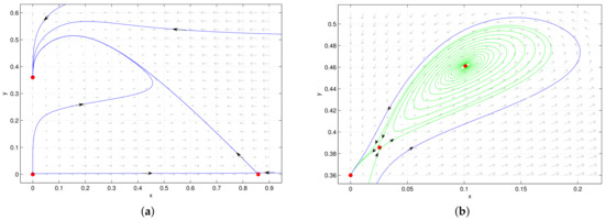
Thus, system (2) can undergo subcritical Hopf bifurcation, supercritical Hopf bifurcation and degenerate Hopf bifurcation of codimension 2 (Figure 1 and Figure 2). Further, we obtain the following theorem.

Figure 1. (a) An unstable limit cycle generated by the subcritical Hopf bifurcation of system (2) with $a={\displaystyle \frac{1}{5}}$, $h={\displaystyle \frac{116}{375}}-0.00013$, $q={\displaystyle \frac{1}{5}}$, $s={\displaystyle \frac{7}{240}}$ and $k={\displaystyle \frac{1}{10}}$. (b) A stable limit cycle generated by the supcritical Hopf bifurcation of system (2) with $a=1$, $h={\displaystyle \frac{1}{5}}+0.00015$, $q={\displaystyle \frac{1}{5}}$, $s={\displaystyle \frac{1}{20}}$ and $k={\displaystyle \frac{1}{10}}$.

Figure 2. Two limit cycles (the inner is stable) generated by the degenerate Hopf bifurcation of system (2) with $a={\displaystyle \frac{117}{37}}+0.03784$, $h={\displaystyle \frac{297}{7400}}-0.00056$, $q={\displaystyle \frac{1}{20}}$, $s={\displaystyle \frac{29}{370}}$ and $k={\displaystyle \frac{1}{10}}$.

Theorem 6.

Assume that (20) and (21) hold, and

(1)

If $l_1\ne 0$, then $E_{12}$ is a weak focus of order 1;

(2)

If $l_1=0$ and $l_2\ne 0$, then $E_{12}$ is a weak focus of order 2;

(3)

If $l_1=0$ and $l_2=0$, then $E_{12}$ is a weak focus of at least order 3.

From the above examples, we know that conclusions (1) and (2) of Theorem 6 are true. Next, inspired by the method in [26,38], we verify conclusion (3) of Theorem 6, especially the existence of the degenerate Hopf bifurcation of codimension 3.

For the polynomials $f,g$ and $g_i$$(i=1,2,\dots ,n)$, let $V(g_1,g_2,\dots ,g_n)$ be the set of common zeros of $g_i$$(i=1,2,\dots ,n)$, $\mathrm{res}(f,g,x)$ be the Sylvester resultant of f and g with respect to x, $\mathrm{lcoeff}(f,x)$ be the leading coefficient of f with respect to x, and $\mathrm{prem}(f,g,x)$ be the pseudo-remainder of f with respect to g in x.

Let $k={\displaystyle \frac{9}{25}}$ and $z={\displaystyle \frac{3}{25}}$. Also, from $f\left(z\right)=0$ and $\mathrm{Tr}\left(J_{E_z}\right)=0$, we have

$$\begin{array}{c}{\displaystyle h=\overline{h}:=-\frac{2(25q+3)(6a-11)}{625},s=\overline{s}:=-\frac{3(12a+25q-19)}{25(25q+3)}.}\hfill \end{array}$$

(24)

By $h>0,s>0$ and $\mathrm{Det}\left(J_{E_z}\right)>0$, we define

$$\begin{array}{c}{\mathcal{M}}_{*}:=\left\{{\displaystyle (a,q)\in {\mathbb{R}}_{+}^2|\frac{19-25q}{25q+15}<a<\frac{19-25q}{12},0<q<\frac{19}{25}}\right\}.\hfill \end{array}$$

(25)

We can obtain the following theorem.

Theorem 7.

When $(a,h,q,s,k,z)=\left(-{\displaystyle \frac{{\chi }_2\left(q\right)}{{\chi }_1\left(q\right)}},\overline{h},q_6,\overline{s},{\displaystyle \frac{9}{25}},{\displaystyle \frac{3}{25}}\right)$, (24) and (25) hold, $E_z$ is a weak focus of order 3 and system (2) can undergo a degenerate Hopf bifurcation of codimension 3 near $E_z$, where ${\chi }_1\left(q\right)$ and ${\chi }_2\left(q\right)$ are given in Appendix B, and $q_6$ is the unique real root of ${\mathcal{R}}_2$ for $(a,q)\in {\mathcal{M}}_{*}$, with ${\mathcal{R}}_2$ being given in (26).

Proof. 

By a series of transformations similarly to (22), by computation, we obtain the first three Lyapunov coefficients

$$\begin{array}{c}{\displaystyle L_1^{*}=-\frac{324a{l}_1^{*}}{6103515625(25q+3)D_{*}^{3/2}},}\hfill \\ {\displaystyle L_2^{*}=\frac{486a{l}_2^{*}}{2384185791015625{(25q+3)}^3(19-12a-25q)D_{*}^{5/2}},}\hfill \\ {\displaystyle L_3^{*}=\frac{118098a{l}_3^{*}}{227373675443232059478759765625{(25q+3)}^5(19-12a-25q)D_{*}^{9/2}},}\hfill \end{array}$$

where

$$\begin{array}{ccc}{l}_1^{*}\hfill & =& (187500q^3-67500q^2-56700q-324)a^2+(390625q^4+218750q^3-7500q^2\hfill \\ \hfill & & +202050q+5643)a+390625q^4-500000q^3+336250q^2-172200q-9027,\hfill \\ D_{*}\hfill & =& {\displaystyle \frac{1296}{244140625}(25aq+15a+25q-19)(19-12a-25q),}\hfill \end{array}$$

$l_2^{*}$ is given in Appendix B, and the expression of $l_3^{*}$ is omitted here.

Notice that

$$V(L_1^{*},L_2^{*},L_3^{*})\cap {\mathcal{M}}_{*}=V(l_1^{*},l_2^{*},l_3^{*})\cap {\mathcal{M}}_{*}.$$

Next, we prove that $L_i^{*}(i=1,2,3)$ have no common zero for $(a,q)\in {\mathcal{M}}_{*}$, that is $V(l_1^{*},l_2^{*},l_3^{*})\cap {\mathcal{M}}_{*}=\varnothing ;$ thus, $E_z$ is a weak focus of order at most 3 for $(a,q)\in {\mathcal{M}}_{*}$.

By computation, we can obtain

$$\begin{array}{c}{r}_{12}=\mathrm{res}(l_1^{*},l_2^{*},a)=-41421570048(625q^2-400q+147){(25q+3)}^{12}{\mathcal{R}}_1{\mathcal{R}}_2,\hfill \\ r_{13}=\mathrm{res}(l_1^{*},l_3^{*},a)=-1401753648073015296(625q^2-400q+147){(25q+3)}^{20}{\mathcal{R}}_1{\mathcal{R}}_3,\hfill \end{array}$$

where

$$\begin{array}{ccc}{\mathcal{R}}_1\hfill & =& 3125q^2-2450q+201,\hfill \\ {\mathcal{R}}_2\hfill & =& 104308128356933593750q^{13}-58591365814208984375q^{12}\hfill \\ \hfill & & -369558334350585937500q^{11}+640571212768554687500q^{10}\hfill \\ \hfill & & -518147544860839843750q^9+252848341827392578125q^8\hfill \\ \hfill & & -34858674755859375000q^7-17523764964843750000q^6\hfill \\ \hfill & & +3731709216972656250q^5-272165283636328125q^4\hfill \\ \hfill & & +26524129048312500q^3-1899706172017500q^2\hfill \\ \hfill & & +44533906478550q-40216679577,\hfill \end{array}$$

(26)

and the expression of ${\mathcal{R}}_3$ is too long and is omitted. Since $(625q^2-400q+147)(25q+3)$ is nonzero for $q>0$, from Lemma 2 in Chen and Zhang [39], we have

$$\begin{array}{c}V(l_1^{*},l_2^{*},l_3^{*})=V(l_1^{*},l_2^{*},l_3^{*},\mathrm{lcoeff}(l_1^{*},a))\cup V\left({\displaystyle \frac{l_1^{*},l_2^{*},l_3^{*},r_{12},r_{13}}{\mathrm{lcoeff}(l_1^{*},a)}}\right).\hfill \end{array}$$

(27)

Note that $\mathrm{lcoeff}(l_1^{*},a)=187500q^3-67500q^2-56700q-324<0$ for $q\in (0,{\displaystyle \frac{19}{25}})$. Again, from Lemma 2 in Chen Zhang [39], there is

$$V(r_{12},r_{13})=V\left({\mathcal{R}}_1\right)\cup V({\mathcal{R}}_2,{\mathcal{R}}_3),$$

then it follows from (27) that

$$V(l_1^{*},l_2^{*},l_3^{*})\cap {\mathcal{M}}_{*}=V_1\cup V_2,$$

where

$$\begin{array}{c}{V}_1=V(l_1^{*},l_2^{*},l_3^{*},{\mathcal{R}}_1)\cap {\mathcal{M}}_{*},V_2=V(l_1^{*},l_2^{*},l_3^{*},{\mathcal{R}}_2,{\mathcal{R}}_3)\cap {\mathcal{M}}_{*}.\hfill \end{array}$$

First, we prove that $V(l_1^{*},l_2^{*},l_3^{*})\cap {\mathcal{M}}_{*}=\varnothing$ by two steps.

Step 1. Proving that $V_1=\varnothing$. If ${\mathcal{R}}_1=0$, then

$$q_1={\displaystyle \frac{49-2\sqrt{349}}{125}},q_2={\displaystyle \frac{49+2\sqrt{349}}{125}}.$$

When $q=q_1$, we have

$$l_1^{*}={\displaystyle \frac{8(10363-134\sqrt{349})(179778a-2983055+133841\sqrt{349})(-30a+23+\sqrt{349})}{56180625}}<0,$$

for $a\in \left({\displaystyle \frac{355+17\sqrt{349}}{699}},{\displaystyle \frac{23+\sqrt{349}}{30}}\right)$.

Similarly, when $q=q_2$, we can obtain $l_1^{*}<0$, for $a\in \left({\displaystyle \frac{355-17\sqrt{349}}{699}},{\displaystyle \frac{23-\sqrt{349}}{30}}\right)$. Thus, $V(l_1^{*},{\mathcal{R}}_1)=\varnothing$, which implies $V_1=\varnothing$.

Step 2. Proving that $V_2=\varnothing$. By computation, we have $\mathrm{res}({\mathcal{R}}_2,{\mathcal{R}}_3,q)>0$, which is given in Appendix B. Then, $V({\mathcal{R}}_2,{\mathcal{R}}_3)=\varnothing$, which implies $V_2=\varnothing$.

Next, we prove $V(l_1^{*},l_2^{*})\cap {\mathcal{M}}_{*}\ne \varnothing$; that is, $E_z$ is a weak focus of exactly order 3 under the conditions of the theorem and ${\mathcal{R}}_2=0$. In the interval $(0,{\displaystyle \frac{19}{25}})$, ${\mathcal{R}}_2$ has five real zeros

$$\begin{array}{c}{q}_3\doteq 0.0009402819090,q_4\doteq 0.04064618715,q_5\doteq 0.05905768722;\hfill \\ q_6\doteq 0.1357064321,q_7\doteq 0.5678998990.\hfill \end{array}$$

When $q=q_6$, we find that

$$l_1^{*}=-8793.050303a^2+33603.54669a-27320.30568$$

has a unique real zero in $\left({\displaystyle \frac{19-25q_6}{25q_6+15}},{\displaystyle \frac{19-25q_6}{12}}\right)$. Similarly, we can easily verify that when $q=q_3,q_4,q_5$ or $q_7$, $l_1^{*}$ has a nonzero in ${\mathcal{M}}_{*}$. Thus, ${\mathcal{R}}_2$ has a unique real zero $q=q_6$ in ${\mathcal{M}}_{*}$. Using the Maple command “realroot”, we have

$$q_6\in I=\left[{\displaystyle \frac{80106938296210183713}{590295810358705651712}},{\displaystyle \frac{640855506369681469705}{4722366482869645213696}}\right]\subset \left(0,{\displaystyle \frac{19}{25}}\right).$$

In the following, we give the relationship of a and q. By computation we have

$$w:=\mathrm{prem}(l_2^{*},l_1^{*},a)=-20736{(25q+3)}^4({\chi }_1\left(q\right)a+{\chi }_2\left(q\right)),$$

where ${\chi }_1\left(q\right)$ and ${\chi }_2\left(q\right)$ are presented in Appendix B. Notice that

$$\mathrm{lcoeff}(l_1^{*},a)=187500q^3-67500q^2-56700q-324<0,\mathrm{for}q\in \left(0,{\displaystyle \frac{19}{25}}\right).$$

According to Sturm’s theorem, ${\chi }_1\left(q\right)\ne 0$ for all $q\in I$. Obviously, ${\mathcal{R}}_2=0$ implies $l_1^{*}=0$, which together with $w=0$ lead to $l_2^{*}=0$. Thus, from $w=0$, we can obtain

$$a=\overline{a}:=-{\displaystyle \frac{{\chi }_2\left(q\right)}{{\chi }_1\left(q\right)}}.$$

By Sturm’s theorem again, we can obtain ${\left(-{\displaystyle \frac{{\chi }_2\left(q\right)}{{\chi }_1\left(q\right)}}\right)}^{\prime }<0$ for $q\in I$. Then, $-{\displaystyle \frac{{\chi }_2\left(q\right)}{{\chi }_1\left(q\right)}}$ is a strictly decreasing function in I. By computation, we can easily verify that

$$a\in (1.1731509453,1.1731509455)\subset \left({\displaystyle \frac{19-25q}{25q+15}},{\displaystyle \frac{19-25q}{12}}\right),\mathrm{for}q\in I.$$

Therefore,

$$V(L_1^{*},L_2^{*})\cap {\mathcal{M}}_{*}=V(l_1^{*},l_2^{*},r_{12})\cap {\mathcal{M}}_{*}\ne \varnothing .$$

Finally,

$${\left|{\displaystyle \frac{\partial (\mathrm{Tr}\left(J_{E_z}\right),L_1^{*},L_2^{*})}{\partial (a,q,z)}}\right|}_{(k,z)=({\displaystyle \frac{9}{25}},{\displaystyle \frac{3}{25}})}={\displaystyle \frac{6103515625aJ(a,q)}{107495424{(25aq+15a+25q-19)}^5{(12a+25q-19)}^6{(25q+3)}^6}},$$

where the expression of $J(a,q)$ is too long and is omitted here. Obviously,

$${(25aq+15a+25q-19)}^5{(12a+25q-19)}^6{(25q+3)}^6>0,\mathrm{for}(a,q)\in {\mathcal{M}}_{*},$$

and

$$\mathrm{res}({\mathcal{R}}_2,J(a,q),q)=J_0\left(a\right),$$

where $J_0\left(a\right)$ is a polynomial in a of degree 130, whose expression is omitted. □

Using the Maple command “realroot$(J_0\left(a\right),{10}^{-9})$”, there is $J_0\left(a\right)\ne 0$ for $a\in (1.1731509453,1.1731509455)$. Hence, $\left|{\displaystyle \frac{\partial (\mathrm{Tr}\left(J_{E_z}\right),L_1^{*},L_2^{*})}{\partial (a,q,z)}}\right|\ne 0$, for $(a,q,k,z)=(\overline{a},q_6,{\displaystyle \frac{9}{25}},{\displaystyle \frac{3}{25}})$. Therefore, system (2) can undergo a degenerate Hopf bifurcation of codimension 3 near $E_z$, if $(a,h,q,s,k,z)=\left(-{\displaystyle \frac{{\chi }_2\left(q\right)}{{\chi }_1\left(q\right)}},\overline{h},q_6,\overline{s},{\displaystyle \frac{9}{25}},{\displaystyle \frac{3}{25}}\right)$.

4. Numerical Simulations

In this section, we give some numerical simulations to verify the bifurcation phenomena of system (2) and discuss the influence of the nonlinear harvesting on the dynamic behaviors of system (2).

4.1. Bifurcation Diagrams and Phase Portraits

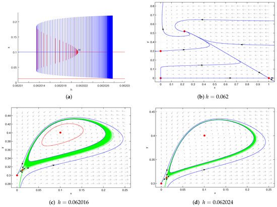
According to Theorem 7, the positive equilibrium $E_{12}$ can be a weak focus of order 3, and system (2) can undergo a degenerate Hopf bifurcation of codimension 3 near $E_{12}$. This means system (2) can admit three limit cycles when there are some small perturbations of the system’s parameters, which can lead to the tristability of the system.

We fix

$$(a,q,s,k)=(1.173,0.13538,0.028,0.36),$$

and give the bifurcation diagram in Figure 3a. We find that system (2) admits three limit cycles when $h\in (0.080781608,0.080781722)$, where the middle limit cycle is unstable and the other two limit cycles are stable, whose phase portrait is shown in Figure 3b. This means that the triple-stability of system (2) may occur. This phenomenon verifies the feasibilities of Theorems 6 and 7.

Figure 3. Fix $(a,q,s,k)=(1.173,0.13538,0.028,0.36)$. (a) Bifurcation diagram of system (2) in the $(h,x)$ plane, where the blue and red lines, respectively, represent stable and unstable limit cycles or equilibrium. (b) Three limit cycles with $h=0.08078165$.

According to Theorem 5, system (2) can undergo a degenerate Bogdanov–Takens bifurcation of codimension 4 around $E_{*}$. More precisely, there exist degenerate Bogdanov–Takens bifurcations of codimension 2 or 3. To verify these results, fixing

$$(a,s,k)=(0.93,0.045,0.36),$$

we obtain a two-parameters bifurcation diagram of the cusp-type Bogdanov–Takens bifurcation of system (2) in the $(h,q)$ plane, as shown in Figure 4. The bifurcation curves divide the $(h,q)$ plane into six regions, and system (2) undergoes different dynamical behaviors in regions I–VI of Figure 4. The corresponding phase portraits are presented in Figure 5, while the detail dynamical behaviors are shown in Table 1. By numerical simulations, we find that system (2) undergoes saddle-node bifurcation, homoclinic bifurcation, subcritical and supercritical Hopf bifurcation, and saddle-node bifurcation of limit cycles; further, the coexistence of the two species is possible.

Figure 4. (a) Bifurcation diagram of system (2) in $(h,q)$ plane with $(a,s,k)=(0.93,0.045,0.36)$. (b) The local enlarged view of (a). $GH$ and $BT$ are the degenerate Hopf bifurcation point and Bogdanov–Takens bifurcation point, respectively. The blue, magenta, green and red solid curves, respectively, denote the Hopf bifurcation, saddle-node bifurcation, saddle-node bifurcation of limit cycles and homoclinic bifurcation.

Figure 5. Phase portraits of system (2) with $(a,s,k)=(0.93,0.045,0.36)$. (a) $(h,q)=(0.15,0.2)\in \mathrm{region}\mathrm{I}$. (b) $(h,q)=(0.15,0.218)\in \mathrm{region}\mathrm{II}$. (c) $(h,q)=(0.15,0.219)\in \mathrm{region}\mathrm{III}$. (d) $(h,q)=(0.15,0.22)\in \mathrm{region}\mathrm{IV}$. (e) $(h,q)=(0.13901,0.19954)\in \mathrm{region}\mathrm{V}$. (f) $(h,q)=(0.13814,0.19796)\in \mathrm{region}\mathrm{VI}$. The detailed dynamical behaviors appear in Table 1.

Table 1. Dynamical behaviors of system (2) in regions I–VI of Figure 4.

Region	${\mathit{E}}_{11}$	${\mathit{E}}_{12}$	Limit Cycles
I	-	-	No (see Figure 5a)
II	saddle	unstable focus	No (see Figure 5b)
III	saddle	unstable focus	A stable limit cycle (see Figure 5c)
IV	saddle	stable focus	No (see Figure 5d)
V	saddle	unstable focus	Two limit cycles (the inner is stable) (see Figure 5e)
VI	saddle	stable focus	An unstable limit cycle (see Figure 5f)

4.2. The Impact of Harvesting on the System

To discuss the impact of the nonlinear harvesting on the dynamic behaviors of system (2), we fix

$$(a,q,s,k)=(1.5,0.107,0.0444,0.3),$$

and present the bifurcation diagram in the $(h,x)$ plane in Figure 6a.

Figure 6. Fix $(a,q,s,k)=(1.5,0.107,0.0444,0.3)$. (a) Bifurcation diagram of system (2) in $(h,x)$ plane, where the blue and red lines, respectively, represent stable and unstable limit cycles or equilibrium. (b–f) Phase portraits of system (2) with different values of h.

When $h=0$, the unique positive equilibrium of system (2) without harvesting is globally asymptotically stable. When $h<0.06201343$, this dynamic behavior does not change (Figure 6b). When $0.06201343<h<0.06202117$, there exist two limit cycles, where the inner is unstable and the outer is stable (Figure 6c). When $0.06202117<h<0.06202771$, the unstable limit cycle disappears and the amplitude of the stable limit cycle continues to increase (Figure 6d). As h continues to increase, the unstable positive equilibrium (Figure 6e) will disappear, and all the solutions of system (2) converge to the boundary equilibrium $E_1(0,0.3)$ (Figure 6f). Hence, if h is relatively small, the system will be stable in fixed sizes ($E_{12}$ or $E_1$) or in a periodic orbit, which is determined by the initial values, but if h is large enough, the prey will die out while the predator can survive. That means that the over-harvesting is detrimental to the survival of the prey and will eventually lead to the extinction of the prey. Thus, the nonlinear harvesting enriches the dynamic behaviors of system (2), where we classify the different possible types of equilibrium states in Table 2 based on the local stability and bifurcation phenomena of all the equilibria shown in Figure 3 and Figure 5.

Table 2. The classification of the phase portraits of system (2).

Stability	Equilibrium and Limit Cycle State	Figure
Monostability	Single equilibrium	Figure 5a,b
		Figure 6b,e,f
Bistability	Two stable equilibria	Figure 5d
	Equilibrium and a stable limit cycle	Figure 5c and Figure 6d
	Equilibrium and two limit cycles	Figure 5e
	Two sable equilibria and an unstable limit cycle	Figure 5f
Tristability	Equilibrium and three limit cycles	Figure 3b
	Two stable equilibria and two limit cycles	Figure 6c

5. Conclusions

In this paper, we consider a Leslie–Gower predator–prey model with nonlinear harvesting and a generalist predator, which has at most four boundary equilibria and at most two positive equilibria. We can see from Theorem 1 and Lemma 1 that the boundary equilibria $E_0(0,0)$, $E_{10}(x_{10},0)$, $E_{20}(x_{20},0)$ and ${\tilde{E}}_{*}({\displaystyle \frac{1-q}{2}},0)$ are unstable in the first quadrant if they exist. From Theorem 2, the boundary equilibrium $E_1(0,k)$ is stable if h is large enough. From Theorem 3, the unique positive equilibrium $E_{*}(x_{*},y_{*})$ is a cusp of codimension up to 4 and system (2) admits the cusp-type degenerate Bogdanov–Takens bifurcation of codimension 4 around $E_{*}$ according to Theorem 5. It follows from Theorem 7 that the positive equilibrium $E_{12}$ is a weak focus of order 3 and system (2) can undergo a degenerate Hopf bifurcation of codimension 3 near $E_{12}$. Further, using numerical simulation, we show that system (2) has three limit cycles (see Figure 3b).

When $h=0$, that is system (2) without harvesting, Gonzalez-Olivares and Rojas-Palma [34] showed that the system has no periodic solution and the unique positive equilibrium is globally asymptotically stable if it exists. But when considering the system with harvesting, we show that system (2) with $h>0$ has at most two positive equilibria. When $k=0$, that is system (2) with a specialist predator, Gupta, Banerjee and Chandra [31] showed that the system undergoes subcritical and supercritical Hopf bifurcation by calculating the first Lyapunov number, and they proved that the origin is an attractor point if the harvesting is large, which means that the prey will be extinct due to the over-harvesting and so will the predator due to the lack of prey. This phenomenon will be changed by considering the generalist predator. When h is large enough, in this paper, we show that system (2) with $k>0$ has no positive equilibrium and the boundary equilibrium $E_1(0,k)$ is globally stable. That is, all the solutions will converge to $E_1(0,k)$, which is consistent with an ecological phenomenon: Harvesting could change the balance of the ecosystem; especially, the over-harvesting can lead to the extinction of the prey, but the predator will remain stable because of the other food sources. Therefore, the over-harvesting is detrimental to the survival of the prey, and the generalist predator provides some protection for the predator in the absence of the prey. Further, different from the dynamic behaviors of system (2) with $k=0$, in which the system undergoes a Bogdanov–Takens bifurcation of codimension 2 or 3 obtained by Refs. [32,33], when considering the influence of a generalist predator, we prove that system (2) undergoes a degenerate Bogdanov–Takens bifurcation of codimension 4 and a degenerate Hopf bifurcation of codimension 3, which can lead to multistable phenomena by some small perturbations of parameters, and system (2) can exist three in types of stable states, that is monostability, bistability and tristability in a biological system (shown in Table 2). For example, Figure 5e implies bistability—that is when the initial values (i.e., the initial densities of both populations) lie inside the outer limit cycle, the predator and prey will coexist oscillatorily on the inner limit cycle. When the initial values lie outside the outer limit cycle, the prey will be extinct and the predator will survive. Also, Figure 3b implies the tristability—that is, when the initial values lie inside the middle limit cycle, the predator and the prey will coexist oscillatorily on the inner limit cycle. When the initial values lie inside the region between two stable invariant manifolds of the saddle, the predator and the prey will coexist oscillatorily on the outer limit cycle. When the initial values lie outside the above regions, the prey will be extinct, and the predator will survive. Therefore, the generalist predator and the nonlinear harvesting enrich the dynamic behaviors of system (2). Based on the ecological environment and significance, we can control the initial densities of both populations to determine whether the population is periodic coexistence or extinction.

Garain and Mandal [40] found that the component Allee effect makes the system appear more complex and have more interesting dynamics; thus, for system (1) with an Allee effect on prey, there may be richer dynamic behaviors, which can be studied in the future.

References

- Lotka, A.J. A natural population norm. J. Wash. Acad. Sci. 1913, 3, 241–248. [Google Scholar]
- Volterra, V. Fluctuations in the abundance of a species considered mathematically. Nature 1926, 118, 558–560. [Google Scholar] [CrossRef]
- Holling, C.S. The functional response of predators to prey density and its role in mimicry and population regulation. Mem. Entomol. Soc. Can. 1965, 45, 1–60. [Google Scholar] [CrossRef]
- Yao, Y.; Liu, L.L. Dynamics of a predator–prey system with foraging facilitation andgroup defense. Commun. Nonlinear Sci. Numer. Simul. 2024, 138, 108198. [Google Scholar] [CrossRef]
- Zhang, H.S.; Cai, Y.L.; Fu, S.M.; Wang, W.M. Impact of the fear effect in a prey-predator model incorporating a prey refuge. Appl. Math. Comput. 2019, 356, 328–337. [Google Scholar] [CrossRef]
- Bai, D.Y.; Wu, J.H.; Zheng, B.; Yu, J.S. Hydra effect and global dynamics of predation with strong Allee effect in prey and intraspecific competition in predator. J. Differ. Equations 2024, 384, 120–164. [Google Scholar] [CrossRef]
- Wu, S.H.; Song, Y.L. Stability analysis of a diffusive predator–prey model with Hunting cooperation. J. Nonlinear Model. Anal. 2021, 3, 321–334. [Google Scholar]
- Yuan, P.; Chen, L.; You, M.S.; Zhu, H.P. Dynamics complexity of generalist predatory mite and the Leafhopper pest in tea plantations. J. Dyn. Differ. Equations 2023, 35, 2833–2871. [Google Scholar] [CrossRef]
- Leslie, P.H. Some further notes on the use of matrices in population mathematics. Biometrika 1948, 35, 213–245. [Google Scholar] [CrossRef]
- Leslie, P.H. A stochastic model for studying the properties of certain biological systems by numerical methods. Biometrika 1958, 45, 16–31. [Google Scholar] [CrossRef]
- Pielou, E.C. Mathematical Ecology, 2nd ed.; John Wiley & Sons: New York, NY, USA, 1977. [Google Scholar]
- Korobeinikov, A. A Lyapunov function for Leslie–Gower predator–prey models. Appl. Math. Lett. 2001, 14, 697–699. [Google Scholar] [CrossRef]
- Tanner, J.T. The stability and the intrinsic growth rates of prey and predator populations. Ecology 1975, 56, 855–867. [Google Scholar] [CrossRef]
- Hsu, S.B.; Huang, T.W. Global stability for a class of predator–prey system. SIAM J. Appl. Math. 1995, 55, 763–783. [Google Scholar] [CrossRef]
- Huang, J.C.; Ruan, S.G.; Song, J. Bifurcations in a predator–prey system of Leslie type with generalized Holling type III functional response. J. Differ. Equations 2014, 257, 1721–1752. [Google Scholar] [CrossRef]
- Dai, Y.F.; Zhao, Y.L.; Sang, B. Four limit cycles in a predator–prey system of Leslie type with generalized Holling type III functional response. Nonlinear Anal. Real World Appl. 2019, 50, 218–239. [Google Scholar] [CrossRef]
- He, M.X.; Li, Z. Global dynamics of a Leslie–Gower predator–prey model with square root response function. Appl. Math. Lett. 2023, 140, 108561. [Google Scholar] [CrossRef]
- Aziz-Alaoui, M.A.; Okiye, M.D. Boundedness and global stability for a predator–prey model with modified Leslie–Gower and Holling-type II schemes. Appl. Math. Lett. 2003, 16, 1069–1075. [Google Scholar] [CrossRef]
- Xiang, C.; Huang, J.C.; Wang, H. Linking bifurcation analysis of Holling-Tanner model with generalist predator to a changing environment. Stud. Appl. Math. 2022, 49, 124–163. [Google Scholar] [CrossRef]
- Lu, M.; Huang, J.C.; Wang, H. An organizing center of codimension four in a predator–prey model with generalist predator: From tristability and quadristability to transients in a nonlinear environmental change. SIAM J. Appl. Dyn. Syst. 2023, 22, 694–729. [Google Scholar] [CrossRef]
- He, M.X.; Li, Z. Dynamics of a Lesile-Gower predator–prey model with square root response function and generalist predator. Appl. Math. Lett. 2024, 157, 109193. [Google Scholar] [CrossRef]
- Chen, M.M.; Takeuchi, Y.; Zhang, J.F. Dynamic complexity of a modified Leslie–Gower predator–prey system with fear effect. Commun. Nonlinear Sci. Numer. Simul. 2023, 119, 107109. [Google Scholar] [CrossRef]
- Feng, X.Z.; Liu, X.; Sun, C.; Jiang, Y.L. Stability and Hopf bifurcation of a modified Leslie–Gower predator–prey model with Smith growth rate and B-D functional response. Chaos Solitons Fractals 2023, 174, 113794. [Google Scholar] [CrossRef]
- Clark, C.W. Mathematical Bioeconomics, The Optimal Management of Renewable Resources, 2nd ed.; John Wiley and Sons: New York, NY, USA; Toronto, ON, Canada, 1990. [Google Scholar]
- Huang, J.C.; Gong, Y.J.; Ruan, S.G. Bifurcations analysis in a predator–prey model with constant-yield predator harvesting. Discret. Contin. Dyn. Syst. Ser. B 2013, 18, 2101–2121. [Google Scholar] [CrossRef]
- Xiang, C.; Lu, M.; Huang, J.C. Degenerate Bogdanov–Takens bifurcation of codimension 4 in Holling-Tanner model with harvesting. J. Differ. Equations 2022, 314, 370–417. [Google Scholar] [CrossRef]
- Wu, H.; Li, Z.; He, M.X. Bifurcation analysis of a Holling-Tanner model with generalist predator and constant-yield harvesting. Int. J. Bifurc. Chaos 2024, 34, 2450076. [Google Scholar] [CrossRef]
- Xu, Y.C.; Yang, Y.; Meng, F.W.; Ruan, S.G. Degenerate codimension-2 cusp of limit cycles in a Holling-Tanner model with harvesting and anti-predator behavior. Nonlinear Anal. Real World Appl. 2024, 76, 103995. [Google Scholar] [CrossRef]
- García, C. Bifurcations on a discontinuous Leslie-Grower model with harvesting and alternative food for predators and Holling II functional response. Commun. Nonlinear Sci. Numer. Simul. 2023, 116, 106800. [Google Scholar] [CrossRef]
- Zhu, C.R.; Lan, K.Q. Phase portraits, Hopf bifurcations and limit cycles of Leslie–Gower predator–prey systems with harvesting rates. Discret. Contin. Dyn. Syst. Ser. B 2010, 14, 289–306. [Google Scholar]
- Gupta, R.P.; Banerjee, M.; Chandra, P. Bifurcation analysis and control of Leslie–Gower predator–prey model with Michaelis-Menten type prey-harvesting. Differ. Equations Dyn. Syst. 2012, 20, 339–366. [Google Scholar] [CrossRef]
- Kong, L.; Zhu, C.R. Bogdanov–Takens bifurcations of codimensions 2 and 3 in a Leslie–Gower predator–prey model with Michaelis–Menten–type prey harvesting. Math. Methods Appl. Sci. 2017, 40, 6715–6731. [Google Scholar] [CrossRef]
- Yao, J.H.; Huzak, R. Cyclicity of the limit periodic sets for a singularly perturbed Leslie–Gower predator–prey model with prey harvesting. J. Dyn. Differ. Equations 2024, 36, 1721–1758. [Google Scholar] [CrossRef]
- Gonzalez-Olivares, E.; Rojas-Palma, A. Global stability in a modified Leslie–Gower type predation model assuming mutual interference among generalist predators. Math. Biosci. Eng. 2020, 17, 7708–7731. [Google Scholar] [CrossRef] [PubMed]
- Zhang, Z.F.; Ding, T.R.; Huang, W.Z.; Dong, Z.X. Qualitative Theory of Diffrential Equations; Translation of Mathematical Monographs; American Mathematical Society: Providence, RI, USA, 1992. [Google Scholar]
- Dumortier, F.; Roussarie, R.; Sotomayor, J. Generic 3-parameter families of vector fields on the plane, unfolding a singularity with nilpotent linear part. The cusp case of codimension 3. Ergod. Theory Dyn. Syst. 1987, 7, 375–413. [Google Scholar] [CrossRef]
- Li, C.Z.; Rousseau, C. A system with three limit cycles appearing in a Hopf bifurcation and dying in a homoclinic bifurcation: The cusp of order 4. J. Differ. Equations 1989, 79, 132–167. [Google Scholar] [CrossRef]
- Xiang, C.; Huang, J.C.; Wang, H. Bifurcations in Holling-Tanner model with generalist predator and prey refuge. J. Differ. Equations 2023, 343, 495–529. [Google Scholar] [CrossRef]
- Chen, X.W.; Zhang, W.N. Decomposition of algebraic sets and applications to weak centers of cubic systems. J. Comput. Appl. Math. 2009, 23, 565–581. [Google Scholar] [CrossRef]
- Garain, K.; Mandal, P.S. Bubbling and Hydra Effect in a Population System with Allee Effect. Ecol. Complex. 2021, 47, 100939. [Google Scholar] [CrossRef]
Disclaimer/Publisher’s Note: The statements, opinions and data contained in all publications are solely those of the individual author(s) and contributor(s) and not of MDPI and/or the editor(s). MDPI and/or the editor(s) disclaim responsibility for any injury to people or property resulting from any ideas, methods, instructions or products referred to in the content. |
© 2024 by the authors. Licensee MDPI, Basel, Switzerland. This article is an open access article distributed under the terms and conditions of the Creative Commons Attribution (CC BY) license (https://creativecommons.org/licenses/by/4.0/).